Two-loop Critical Fluctuation-Dissipation Ratio
for the Relaxational Dynamics of the $O(N)$
Landau-Ginzburg Hamiltonian

Abstract

The off-equilibrium purely dissipative dynamics (Model A) of the $O(N)$ vector model is considered at criticality in an $\epsilon=4-d>0$ expansion up to $O(\epsilon^{2})$. The scaling behavior of two-time response and correlation functions at zero momentum, the associated universal scaling functions and the nontrivial limit of the fluctuation-dissipation ratio are determined in the aging regime.

I Introduction

In recent years many efforts have been made in order to understand the off-equilibrium aspects of the dynamics of statistical systems. A variety of novel dynamical behaviors emerges when some kind of randomness is present in the system. Among them, one of the most striking is that of aging (see Ref. [1] and references therein). It has been pointed out [2] that they could also emerge in nondisordered systems if slow-relaxing modes are present. This naturally happens when the system undergoes a second-order phase transition at some critical temperature $T_{c}$. Indeed, consider a ferromagnetic model in a disordered state and quench it to a given temperature $T\geq T_{c}$ [3] at time $t=0$. During the relaxation a small external field $h$ is applied at ${\bf x}=0$ after a waiting time $s$. At time $t$, the order parameter response to $h$ is given by the response function $R_{\bf x}(t,s)=\delta\langle\phi_{\bf x}(t)\rangle/\delta h(s)$, where $\phi$ is the order parameter and $\langle\cdot\rangle$ stands for the mean over the stochastic dynamics. Correlations of order parameter fluctuations are interesting dynamical quantities as well. In the following we will focus on the two-time one, given by $C_{\bf x}(t,s)=\langle\phi_{\bf x}(t)\phi_{\bf 0}(s)\rangle$. The time evolution of the model we are considering is characterized by two different regimes: a transient one with off-equilibrium evolution, for $t<t_{R}$, and a stationary equilibrium evolution for $t>t_{R}$, where $t_{R}$ is the relaxation time. In the former a dependence of the system behavior on initial condition is expected, while in the latter time homogeneity and time reversal symmetry (at least in the absence of external fields) are recovered; as a consequence we expect that for $t_{R}\ll s,t,\;R_{\bf x}(t,s)=R_{\bf x}^{\rm eq}(t-s),\;C_{\bf x}(t,s)=C_{\bf x}^{\rm eq}(t-s)$ where $R_{\bf x}^{\rm eq}$ and $C_{\bf x}^{\rm eq}$ are determined by the “equilibrium” dynamics of the system, with a characteristic time scale diverging at criticality (critical slowing down). Moreover the fluctuation-dissipation theorem states that

$$R_{\bf x}^{\rm eq}(\tau)=-{1\over T}{{\rm d}C_{\bf x}^{\rm eq}(\tau)\over{\rm d}\tau}.$$ (1)

If the system does not reach the equilibrium, all the previous functions will depend both on $s$ (the “age” of the system) and $t$. This behavior is usually referred to as aging and was first predicted for spin glass systems [1, 4]. The fluctuation-dissipation ratio (FDR) [2, 4]:

$$X_{\bf x}(t,s)=\frac{T\,R_{\bf x}(t,s)}{\partial_{s}C_{\bf x}(t,s)}\;,$$ (2)

is usually introduced to measure the distance from the equilibrium of an aging system evolving at a fixed temperature $T$. A non trivial value for this ratio is also experimentally observed in some glassy systems [5].

In recent years several works [1, 2, 4, 6, 7, 8, 9, 10, 11, 12, 13, 14] have been devoted to the study of the FDR for systems exhibiting domain growth [15], and for aging systems such as glasses and spin glasses. $X_{\bf x}(t,s)$ turns out to be a nontrivial function of $t$ and $s$, in the low-temperature phase of all these systems. In particular, analytical and numerical studies indicate that the limit

$$X^{\infty}=\lim_{s\to\infty}\lim_{t\to\infty}X_{{\bf x}=0}(t,s),$$ (3)

vanishes throughout the low-temperature phase both for spin glasses and simple ferromagnetic systems [8, 9, 10, 12, 13].

Only recently [2, 16, 17, 18, 19, 20, 21] attention has been paid to the FDR, for nonequilibrium, nondisordered, and unfrustrated systems at criticality. From general scaling arguments one would expect that the critical response function scales as [19, 20, 21, 22, 23]:

$$R_{\bf x=0}(t,s)={\cal A}_{R}(t-s)^{a-d/z}(t/s)^{\theta}{\cal F}_{R}(s/t)\,,$$ (4)

where $a=(2-\eta-z)/z$ and $\theta$ is the initial-slip exponent of the response function, related to the initial-slip exponent of the magnetization $\theta^{\prime}$ and to the autocorrelation exponent $\lambda_{c}$ [24] by the relation [22]

$$\theta^{\prime}=\theta+z^{-1}(2-z-\eta)=z^{-1}(d-\lambda_{c}).$$ (5)

In recent works the notion of local scale invariance has been introduced as an extension of anisotropic or dynamical scaling (see [25] and references therein). Assuming that the response function transforms covariantly under the constructed group of local transformations, it has been argued [26] that ${\cal F}_{R}(s/t)=1$. Under the same assumption, the full spatial dependence has been also predicted [25]

$$R_{\bf x}(t,s)=R_{\bf x=0}(t,s)\Phi(|{\bf x}|/(t-s)^{1/z}),$$ (6)

where $\Phi(u)$ is a function whose convergent series expansion is explicitly known [25]. For the correlation function and its derivative no analogous prediction exists. One can only expects from general Renormalization Group (RG) arguments that [19, 20, 21, 22, 23]

$$C_{\bf x=0}(t,s) = {\cal A}_{C}(t-s)^{a+1-d/z}(t/s)^{\theta-1}{\cal F}_{C}(s/t)\,,$$ (7)

$$\partial_{s}C_{\bf x=0}(t,s) = {\cal A}_{\partial C}(t-s)^{a-d/z}(t/s)^{\theta}{\cal F}_{\partial C}(s/t)\,,$$ (8)

with the same $\theta$ and $a$ as in Eq. (4). The functions ${\cal F}_{C}(v)$, ${\cal F}_{\partial C}(v)$ and ${\cal F}_{R}(v)$ are universal and defined in such a way ${\cal F}_{C}(0)={\cal F}_{\partial C}(0)={\cal F}_{R}(0)=1$, while the constants ${\cal A}_{C}$, ${\cal A}_{\partial C}$ and ${\cal A}_{R}$ are nonuniversal amplitudes.

From the scaling laws of above, it has been argued that $X^{\infty}$ is a new universal quantity associated with the given nonequilibrium dynamics [19, 17, 20], and, as such, it should attract the same interest as critical exponents. Given this universality, it is worthwhile to compute $X^{\infty}$ for those mesoscopic models of dynamics which have the same critical behavior of some lattice models considered so far in the literature.

Correlation and response functions were exactly computed in the simple cases of a Random Walk, a free Gaussian field, and a two-dimensional $XY$ model at zero temperature and the value $X^{\infty}=1/2$ was found [2]. The analysis of the $d$-dimensional spherical model gave $X^{\infty}=1-2/d$ [17], while $X^{\infty}=1/2$ for the one-dimensional Ising-Glauber chain [16, 19]. Monte Carlo simulations have been done for the two- and three-dimensional Ising model [17], finding $X^{\infty}=0.26(1)$ and $X^{\infty}\simeq 0.40$ respectively. The effect of long-range correlations in the initial configuration has been also analyzed for the $d$-dimensional spherical model [27].

Only in a recent work [21] field-theoretical methods have been applied to determine the FDR and the scaling forms of the response and correlation functions up to the first order in an $\epsilon$ expansion, for the purely relaxational dynamics of the $O(N)$ Ginzburg-Landau model. This field-theoretical model has the same symmetries (and thus the same universal properties) as a wide class of spin systems on the lattice with short range interactions (see [30], or [31] for a recent review).

In [21] the following quantity, related to the FDR, was introduced in momentum space

$${\cal X}_{\bf q}(t,s)={\Omega R_{\bf q}(t,s)\over\partial_{s}C_{\bf q}(t,s)},$$ (9)

where $R_{\bf q}(t,s)$ and $C_{\bf q}(t,s)$ are the Fourier transforms (with respect to ${\bf x}$) of $R_{\bf x}(t,s)$ and $C_{\bf x}(t,s)$ respectively. It was argued that the zero-momentum limit

$${\cal X}_{\bf q=0}^{\infty}=\lim_{s\to\infty}\lim_{t\to\infty}{\cal X}_{\bf q=0}(t,s)$$ (10)

is equal to the same limit of the FDR (3) for ${\bf x=0}$, i.e. ${\cal X}_{\bf q=0}^{\infty}=X^{\infty}$ to all orders [21]. This fact allows an easier perturbative computation in momentum space of the new universal quantity $X^{\infty}$.

The extension of these results to two-loop order is very important not only from a quantitative point of view. In fact, in the past, when new scaling relations have been proposed, several times they resisted to the test of the first order in the $\epsilon$ expansion, but not to higher order calculations. Classical examples may be found in the context of surface criticality (see e.g. the review [28], p. 116, and references therein) and in the case of anisotropic scaling at Lifshitz points [29]. This is a further reason to present here the second order computation of the scaling form for the zero-momentum response function and the FDR for the purely dissipative relaxation of the $O(N)$ model.

The paper is organized as follows. In Sec. II we briefly introduce the model. In Sec. III we evaluate the zero-momentum response function $R_{\bf q=0}(t,s)$ and in particular we derive its scaling form. In Sec. IV we compute the FDR up to the second order in $\epsilon$ and we derive a scaling form for $\partial_{s}C_{\bf q=0}(t,s)$. In Sec. V we summarize and comment our results and discuss some points that need further investigation. In the Appendices A and B we give all the details to compute the zero-momentum Feynman integrals.

II The model

The time evolution of an $N$-component field $\varphi({\bf x},t)$ under a purely dissipative dynamics (Model A of Ref. [32]) is described by the stochastic Langevin equation

$$\partial_{t}\varphi({\bf x},t)=-\Omega\frac{\delta\cal{H}[\varphi]}{\delta\varphi({\bf x},t)}+\xi({\bf x},t)\;,$$ (11)

where $\Omega$ is the kinetic coefficient, $\xi({\bf x},t)$ a zero-mean stochastic Gaussian noise with

$$\langle\xi_{i}({\bf x},t)\xi_{j}({\bf x}^{\prime},t^{\prime})\rangle=2\Omega\,\delta({\bf x}-{\bf x}^{\prime})\delta(t-t^{\prime})\delta_{ij},$$ (12)

and $\cal{H}[\varphi]$ is the static Hamiltonian. It may be assumed, near the critical point, of the Landau-Ginzburg form

$${\cal H}[\varphi]=\int{\rm d}^{d}x\left[\frac{1}{2}(\nabla\varphi)^{2}+\frac{1}{2}r_{0}\varphi^{2}+\frac{1}{4!}g_{0}\varphi^{4}\right].$$ (13)

Instead of solving the Langevin equation for $\varphi(\xi)$ and then averaging over the noise distribution, the equilibrium correlation and response functions can be directly obtained by means of the field-theoretical action [30, 33]

$$S[\varphi,\tilde{\varphi}]=\int{\rm d}t\int{\rm d}^{d}x\left[\tilde{\varphi}\frac{\partial\varphi}{\partial t}+\Omega\tilde{\varphi}\frac{\delta\mathcal{H}[\varphi]}{\delta\varphi}-\tilde{\varphi}\Omega\tilde{\varphi}\right].$$ (14)

Here $\tilde{\varphi}({\bf x},t)$ is an auxiliary field, conjugated to the external field $h$ in such a way that ${\cal H}[\varphi,h]={\cal H}[\varphi]-\int d^{d}xh\,\varphi$. As a consequence, the linear response to the field $h$ of a generic observable ${\cal O}$ is given by

$${\delta\langle{\cal O}\rangle\over\delta h({\bf x},s)}=\Omega\langle\tilde{\varphi}({\bf x},s){\cal O}\rangle\ ,$$ (15)

for this reason $\tilde{\varphi}({\bf x},t)$ is termed response field.

The effect of a macroscopic initial condition $\varphi_{0}({\bf x})=\varphi({\bf x},t=0)$ may be taken into account by averaging over the initial configuration with a weight $e^{-H_{0}[\varphi_{0}]}$ where, for example,

$$H_{0}[\varphi_{0}]=\int\!{\rm d}^{d}x\,\frac{\tau_{0}}{2}(\varphi_{0}({\bf x})-a({\bf x}))^{2},$$ (16)

that specifies an initial state $a({\bf x})$ with gaussian short-range correlations proportional to $\tau_{0}^{-1}$. Any addition of anharmonic terms in $H_{0}[\varphi_{0}]$ is not expected to be relevant as long as the harmonic term is there (as in the case when the initial state is in the high temperature phase). Instead, an initial condition with long-range correlations may lead to a different universality class, as e.g. shown for the $d$-dimensional spherical model with non-conservative dynamics [27].

Following standard methods [30, 33], the response and correlation functions may be obtained by a perturbative expansion of the functional weight $e^{-(S[\varphi,\tilde{\varphi}]+H_{0}[\varphi_{0}])}$ in terms of the coupling constant $g_{0}$ (appearing in the vertex $g_{0}\varphi^{3}\tilde{\varphi}/3!$). The propagators (Gaussian two-point functions of the fields $\varphi$ and $\tilde{\varphi}$) of the resulting theory are [22]

$$\langle\tilde{\varphi_{i}}({\bf q},s)\varphi_{j}(-{\bf q},t)\rangle_{0}= \delta_{ij}R^{0}_{q}(t,s)= \delta_{ij}\,\theta(t-s)G(t-s),$$ (17)

$$\langle\varphi_{i}({\bf q},s)\varphi_{j}(-{\bf q},t)\rangle_{0}= \delta_{ij}C^{0}_{q}(t,s)= {\delta_{ij}\over q^{2}+r_{0}}\left[G(|t-s|)+\left(\frac{r_{0}+q^{2}}{\tau_{0}}-1\right)G(t+s)\right],$$ (18)

where

$$G(t)=\displaystyle{e^{-\Omega(q^{2}+r_{0})t}}.$$ (19)

The response function Eq. (17) is the same as in equilibrium. Eq. (18), instead, reduces to the equilibrium form when both times $t$ and $s$ go to infinity and $\tau=t-s$ is kept fixed. In the following we will assume the Îto prescription (see [23, 34], [30] and references therein) to deal with the ambiguities that arise in formal manipulations of stochastic equations. Consequently, all the diagrams with self-loops of response propagator has to be omitted in the computation. This ensures that causality holds in the perturbative expansion [22, 23, 33]. From the technical point of view, the breaking of time homogeneity makes the renormalization procedure in terms of one-particle irreducible correlation functions less straightforward than in standard cases (see Ref. [28, 22, 23]). Thus the computations will be done in terms of connected functions.

From the expressions above, we can compute the FDR for the Gaussian model [2, 21]:

$${\cal X}_{\bf q}^{0}(t,s)=\left({\partial_{s}C^{0}_{q}\over\Omega R^{0}_{q}}\right)^{-1}=\left(1+e^{-2\Omega(q^{2}+r_{0})s}+\Omega q^{2}\tau_{0}^{-1}e^{-2\Omega(q^{2}+r_{0})s}\right)^{-1}.$$ (20)

When the model is not at its critical point, i.e. $r_{0}\propto T-T_{c}\neq 0$, the limit of this ratio for $s\rightarrow\infty$ is $1$ for all values of $q$, according to the idea that in the high-temperature phase all modes have a finite equilibration time. In this case equilibrium is approached exponentially fast in time and as a consequence the fluctuation-dissipation theorem applies. For the critical model, i.e. $r_{0}=0$, if $q\neq 0$ then the limit ratio is again equal to one, whereas for $q=0$ we have ${\cal X}_{q=0}^{0}(t,s)=1/2$. We can argue that, in the Gaussian model, the only mode characterized by aging, i.e. that “does not relax” to the equilibrium, is the zero mode in the critical limit.

III Two-loop response function

FIG. 1.: Two-loop Feynman diagrams contributing to the response function. Response propagators are drawn as wavy-normal lines, whereas correlators are normal lines. A wavy line is attached to the response field and a normal one to the order parameter.

In this Section we compute, up to the second order in a loop expansion, the critical nonequilibrium response function at zero external momentum for the model described in the previous Section. We use here the method of renormalized field theory in dimensional regularization with minimal subtraction of dimensional poles. Up to the second order in perturbation theory there are four connected Feynman diagrams (without self-loops of response propagator) that contribute to the response function. They are depicted in Figure 1. In terms of these diagrams and as a function of the bare couplings and fields (denoted in the following with $\varphi_{B}$, $\tilde{\varphi}_{B}$), the zero-momentum bare response function $R_{B}(t,s)$ is given by

$$R_{B}(t,s) = R^{0}_{q=0}(t,s)-{N+2\over 6}g_{0}R^{1,1}$$ (22)

$$+g_{0}^{2}\left[\left({N+2\over 6}\right)^{2}R^{2,1}+{(N+2)^{2}\over 18}R^{2,2}+{N+2\over 6}R^{2,3}\right]+O(g_{0}^{3})\;.$$

In the following we assume $t>s$ for simplicity. We also fix $\tau_{0}^{-1}=0$, since $\tau_{0}^{-1}$ is an irrelevant variable (in the RG sense) and thus it affects only the corrections to the leading scaling behavior [22, 23]. Using the results reported in the Appendix A, we get

$$R_{B}(t,s) = 1+\tilde{g}_{0}{N+2\over 24}\left\{\log{t\over s}+{\epsilon\over 2}\left[\left(\gamma_{E}+\log 2+\log t\right)\log{t\over s}-{1\over 2}\log^{2}{t\over s}\right]\right\}+$$ (26)

$${\tilde{g}_{0}^{2}\over 144}\left\{{(N+2)^{2}\over 8}\log^{2}{t\over s}+(N+2)^{2}\left[-\left({1\over\epsilon}+\log 2+\gamma_{E}+\log t\right)\log{t\over s}+{1\over 2}\log^{2}{t\over s}\right]\right\}$$

$$-\tilde{g}_{0}^{2}{N+2\over 24}\left[{1\over\epsilon}\left(\log{4\over 3}+\log{t\over s}\right)+\log{t\over s}\left({1\over 2}+\log t+\gamma_{E}\right)-{1\over 2}\log^{2}{t\over s}\right.$$

$$\left.+(\log(t-s)+\gamma_{E})\log{4\over 3}-{f(s/t)\over 4}\right]+O(g_{0}^{3},g_{0}^{2}\epsilon,g_{0}\epsilon^{2})\,,$$

where $\tilde{g}_{0}=N_{d}g_{0}$, $N_{d}=2/((4\pi)^{d/2}\Gamma(d/2))$ and $f(v)$ is a regular function defined in Eq. (A32). To lighten the notations we set $\Omega=1$ in the previous equations. The dependence on $\Omega$ of final formulas may be simply obtained by $t\mapsto\Omega t$, where $t$ is the generic time variable.

In order to cancel out the dimensional poles appearing in this function, we have to renormalize the coupling constant according to [30]

$$\tilde{g}_{0}=\left(1+{N+8\over 6}{\tilde{g}\over\epsilon}\right)\tilde{g}+O(\tilde{g}^{2}),$$ (27)

and the fields $\varphi$ and $\tilde{\varphi}$ via the relations [33] $\varphi_{B}=Z_{\varphi}^{1/2}\varphi$, $\tilde{\varphi}_{B}=Z_{\tilde{\varphi}}^{1/2}\tilde{\varphi}$, so that

$$R(t,s)=(Z_{\varphi}Z_{\tilde{\varphi}})^{-1/2}R_{B}(t,s)=\left[1+{N+2\over 24}\log{4\over 3}{\tilde{g}^{2}\over\epsilon}+O(\tilde{g}^{3})\right]R_{B}(t,s).$$ (28)

After this renormalization, $R(t,s)$ is a regular function of dimensionality also for $\epsilon\rightarrow 0$. The critical response function is now obtained by fixing $\tilde{g}$ at its fixed point value [30]

$$\tilde{g}^{*}={6\,\epsilon\over N+8}\left[1+{3(3N+14)\over(N+8)^{2}}\epsilon\right]+O(\epsilon^{3})\,,$$ (29)

leading to

$$R(t,s) = 1+\epsilon{N+2\over 4(N+8)}\log{t\over s}+{\epsilon^{2}\over 4}\left[{6(N+2)\over(N+8)^{2}}\left({N+3\over N+8}+\log 2\right)\log{t\over s}+{(N+2)^{2}\over 8(N+8)^{2}}\log^{2}{t\over s}\right.$$ (31)

$$\left.-{6(N+2)\over(N+8)^{2}}\log{4\over 3}\log(t-s)+{3(N+2)\over 2(N+8)^{2}}\left(f(s/t)-4\gamma_{E}\log{4\over 3}\right)\right]+O(\epsilon^{3})\;.$$

Note that the nonscaling terms, like $\log t\log t/s$ (appearing, for example, in $R^{2,3}$, see Eq. (A31)), cancel each other out when the coupling constant is set equal to its fixed point value. Eq. (31) agrees with the expected scaling form in momentum space (analogous to that in real space, Eq. (4))

$$R(t,s)=A_{R}(t-s)^{a}(t/s)^{\theta}F_{R}(s/t)\,,$$ (32)

with the well-known exponents [22, 23, 30]

$$\theta = {N+2\over N+8}{\epsilon\over 4}\left[1+{6\epsilon\over N+8}\left({N+3\over N+8}+\log 2\right)\right]+O(\epsilon^{3})\,,$$ (33)

$$a = {2-\eta-z\over z}=-{3(N+2)\over 2(N+8)^{2}}\log{4\over 3}\,\epsilon^{2}\,+O(\epsilon^{3})\,,$$ (34)

and the nonuniversal amplitude

$$A_{R}=1+\epsilon^{2}{3(N+2)\over 8(N+8)^{2}}\left(f(0)-4\gamma_{E}\log{4\over 3}\right)+O(\epsilon^{3})\,\,.$$ (35)

For the new universal function $F_{R}(v)$ we find

$$F_{R}(v)=1+\epsilon^{2}{3(N+2)\over 8(N+8)^{2}}(f(v)-f(0))+O(\epsilon^{3})\;,$$ (36)

A plot of the quantity $f(v)-f(0)$ (defined in the Appendix A Eq. (A32)), that completely characterizes the out-of-equilibrium corrections to the mean-field behavior up to the second order in the $\epsilon$-expansion, is reported in Fig. 2.

FIG. 2.: Plot of the two-loop contribution to the universal functions $F_{R}(v)$ (see Eq. (36)) and $F_{\partial C}(v)$ (see Eq. (50)).

Due to the small prefactor ($\epsilon^{2}/72$ for the Ising model, $N=1$), it might be very hard to detect these corrections in numerical and experimental works, as it happens for the corrections to the mean-field behavior of the static [31] and equilibrium dynamics [35] two-point functions.

IV Two-loop fluctuation-dissipation ratio

In this Section we evaluate the FDR up to the order $\epsilon^{2}$. We do not compute the full two-point correlation function $C(t,s)$, since only $\partial_{s}C(t,s)$ is required to determine the FDR. This derivative may be computed by using the following diagrammatic identity.

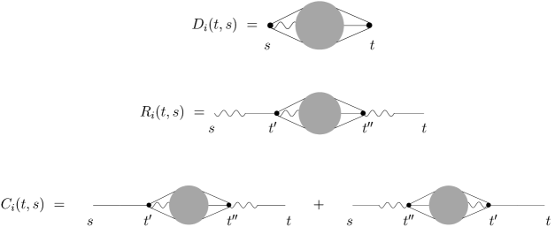
FIG. 3.: Diagrammatic trick.

Each amputated diagram $D_{i}(t,s)$ (with label $i$) contributing to the response function, also contributes to the correlation one in two diagrams, as graphically illustrated in Fig. 3. Taking into account the explicit form of the propagators (see Eqs. (17) and (18)) for $q^{2}=0$ and causality (which also implies that $D_{i}(t,s)\propto\theta(t-s)$ apart from contact terms) it is easy to find that

$$\partial_{s}C_{i}(t,s)=2R_{i}(t,s)+2\int_{0}^{\infty}{\rm d}t^{\prime}\,t^{\prime}D_{i}(t^{\prime},s),$$ (37)

where $C_{i}(t,s)$ is the contribution of this diagram to the correlation function, $R_{i}(t,s)$ the contribution to the response function, and $D_{i}(t^{\prime},s)$ the common amputated part.

FIG. 4.: Diagrams contributing only to the correlation function.

Relation (37) is nothing but a particular case of a relation following an algebraic identity for the functional integral, i. e.

$$0=\int[{\rm d}\varphi{\rm d}\tilde{\varphi}{\rm d}\varphi_{0}]\frac{\delta}{\delta\tilde{\varphi}({\bf x},s)}\left\{\varphi({\bf x}^{\prime},t)e^{-S[\varphi,\tilde{\varphi}]-H_{0}[\varphi_{0}]}\right\}\ ,$$ (38)

with $t>s>0$. At criticality (i.e. $r_{0}=0$, using dimensional regularization) we get in momentum space

$$(\partial_{s}-{\bf q}^{2})\langle\varphi(-{\bf q},t)\varphi({\bf q},s)\rangle=2\langle\varphi(-{\bf q},t)\tilde{\varphi}({\bf q},s)\rangle-\frac{g_{0}}{3!}\langle\varphi(-{\bf q},t)\varphi^{3}({\bf q},s)\rangle\ ,$$ (39)

which, in the limit ${\bf q}^{2}\rightarrow 0$, is diagrammatically expressed by Eq. (37) as far as common amputated contributions to response and correlation functions are concerned.

Diagrams contributing to the correlation function, but not to the response one do exist. They have to be computed without taking advantage of this identity. At two-loop order there are two of them, as in Fig. 4.

Summing the six contributions to the correlation function we finally arrive to the expression:

$${\partial_{s}C_{B}(t,s)\over 2} = R(t,s)-g_{0}{N+2\over 6}(\partial C)^{1,1}_{e}+g_{0}^{2}\left\{\left({N+2\over 6}\right)^{2}(\partial C)^{2,1}_{e}+{(N+2)^{2}\over 18}(\partial C)^{2,2}_{e}\right.$$ (41)

$$\left.+{N+2\over 6}(\partial C)^{2,3}_{e}+{1\over 2}\left[{N+2\over 18}(\partial C)^{2,4}+\left({N+2\over 6}\right)^{2}(\partial C)^{2,5}\right]\right\}+O(g_{0}^{3})\,.$$

Considering the explicit expression for the diagrams given in the Appendix B one obtains the derivative of the bare correlation function. This bare quantity is renormalized using equations (27), (28) and

$$\Omega=Z_{\Omega}\Omega_{B}\qquad\mbox{ with }\qquad Z_{\Omega}=\left({Z_{\varphi}\over Z_{\tilde{\varphi}}}\right)^{1/2}\ ,$$ (42)

so that, taking into account the $\Omega$ we set equal to $1$ in the previous relations,

$$\partial_{s}C(t,s)=Z_{\Omega}Z_{\varphi}^{-1}\,\partial_{s}C_{B}(t,s)=(Z_{\varphi}Z_{\tilde{\varphi}})^{-1/2}\,\partial_{s}C_{B}(t,s)\ .$$ (43)

The expression of $\partial_{s}C(t,s)$ in terms of the renormalized coupling has a multiplicative redefinition of its amplitude at the first order in $\tilde{g}$. Considering the fixed point value for $\tilde{g}$ (cf. Eq. (29)) one finally obtains

$${\partial_{s}C(t,s)\over 2} = \left[1+\epsilon{N+2\over 4(N+8)}+\epsilon^{2}{3(N+2)(3N+14)\over 4(N+8)^{3}}\right]$$ (48)

$$\times\left\{1+\epsilon{N+2\over 4(N+8)}\log{t\over s}+{\epsilon^{2}\over 4}\left[{6(N+2)\over(N+8)^{2}}\left({N+3\over N+8}+\log 2\right)\log{t\over s}+\right.\right.$$

$$\left.\left.{(N+2)^{2}\over 8(N+8)^{2}}\log^{2}{t\over s}-{6(N+2)\over(N+8)^{2}}\log{4\over 3}\log(t-s)\right]\right\}$$

$$\times\Bigg{\{}1+\epsilon^{2}{N+2\over(N+8)^{2}}\left[{3\over 4}\log{4\over 3}\log{t-s\over t+s}-\gamma_{E}{3\over 2}\log{4\over 3}+\Phi(s/t)+{3\over 8}f(s/t)+{N+2\over 8}\right.$$

$$\left.+{3\over 2}\left(1-\log{4\over 3}\right)\log 2-{3\over 4}\left(1+\log{4\over 3}\right)+{3\over 8}\log^{2}{4\over 3}+{3\over 4}{\rm Li_{2}}(1/4)\right]\Bigg{\}}+O(\epsilon^{3})\;,$$

where the function $f(v)$ and $\Phi(v)$ are defined in Eqs. (A32) and (B23) respectively, and ${\rm Li_{2}}$ is the dilogarithmic function whose standard definition is recalled in Eq. (A18). Note that also for $\partial_{s}C(t,s)$ all the nonscaling terms cancel out when the coupling constant is set equal to its fixed point value. This result agrees with the scaling form in momentum space (analogous to Eq. (8))

$$\partial_{s}C(t,s)=A_{\partial C}(t-s)^{a}(t/s)^{\theta}F_{\partial C}(s/t),$$ (49)

with the same $a$ and $\theta$ as given in the previous section and a new universal scaling function $F_{\partial C}(v)$ given by

$$F_{{\partial C}}(v)=1+\epsilon^{2}{3(N+2)\over 8(N+8)^{2}}\left[2\log{4\over 3}\log{1-v\over 1+v}+{8\over 3}(\Phi(v)-\Phi(0))+f(v)-f(0)\right]+O(\epsilon^{3})\,.$$ (50)

A plot of the loop corrections in the above expression (apart from the factor ${3(N+2)\over 8(N+8)^{2}}$ appearing also in $F_{R}(v)$) is shown in Fig. 2. As already noticed for $F_{R}(v)$, effective corrections to mean-field behavior are quantitatively very small for $F_{{\partial C}}(v)$.

Taking the long time limit (according to Eq. (10)) of both the correlation and response functions one obtains the limit of the critical fluctuation-dissipation ratio we are interested in:

$${({\cal X}_{{\bf q}=0}^{\infty})^{-1}\over 2}=1+{N+2\over 4(N+8)}\epsilon+\epsilon^{2}{N+2\over(N+8)^{2}}\left[{N+2\over 8}+{3(3N+14)\over 4(N+8)}+c\right]+O(\epsilon^{3})\,,$$ (51)

with

$$c = -\frac{3}{4}+{3\over 4}\log 2(2+11\log 2-3\log 3)-\frac{23}{8}\log^{2}3$$ (53)

$$+{3\over 2}{\rm Li_{2}}(1/4)-{21\over 4}{\rm Li_{2}}(1/3)+{21\over 8}{\rm Li_{2}}(3/4)-{1\over 8}{\rm Li_{2}}(8/9)=-0.0415\dots\;.$$

We note that the contribution of $c$ to the FDR is quite small. For example, with $N=1$ the sum of the first two terms in brackets is $\sim 1.8$, which is about $45$ times larger than $c$.

V Conclusions and Discussions

In this work we studied the off-equilibrium properties of the purely dissipative relaxational dynamics of an $N$-vector model in the framework of field theoretical $\epsilon$-expansion. The results presented here extend those of Ref. [21]. The scaling forms for the zero-momentum response function and for the derivative with respect to the waiting time of the two-time correlation function read

$$R(t,s) = A_{R}(t-s)^{a}(t/s)^{\theta}F_{R}(s/t)\,,$$ (54)

$$\partial_{s}C(t,s) = A_{\partial C}(t-s)^{a}(t/s)^{\theta}F_{\partial C}(s/t).$$ (55)

The universal functions $F_{R}(s/t)$ and $F_{\partial C}(s/t)$ are given in Eqs. (36) and (50) respectively. In both cases the corrections to the Gaussian value $1$ is of order $\epsilon^{2}$. In principle these corrections should be detectable in computer and experimental works, but being quantitatively very small, they are hard to observe. We would remark that this fact does not mean that aging effects in these models are weak compared with the analogous phenomena in glassy systems. In fact aging manifests itself in the full scaling forms (e.g. $\theta\neq 0$) and in the violation of fluctuation-dissipation theorem, i.e. in $X^{\infty}\neq 1$ in a quantitative way.

We note that the $R(t,s)$ we found agrees with the general RG form, but at first sight it is not compatible with the Fourier transform of Eq. (6). This naïve comparison should be done very carefully because it involves a Fourier integral which could be divergent. The analysis of the full $q$-dependence of $R_{\bf q}(t,s)$ may give some insight into this problem. This dependence has been already carried out up to $O(\epsilon)$ [21], but it is very hard to determine it up to two loops. In other dynamical universality classes this discrepancy already arises at $O(\epsilon)$. The computation of the full $q$-dependence in these cases seems to be simpler and may provide some useful hints [36].

We computed the FDR ${\cal X}_{\bf q=0}$ for general $N$, cf. Eq. (51). As shown in Ref. [21] this quantity for zero momentum has the same long-time limit as the standard FDR $X^{\infty}$. Using this equality we may compare our result with those presented in the literature.

In the limit $N\rightarrow\infty$, Eq. (51) reduces to $X^{\infty}=1/2-\epsilon/8-\epsilon^{2}/32+O(\epsilon^{3})$, in agreement with the exact result for the spherical model $X^{\infty}=1-2/d$ [17].

FIG. 5.: $X^{\infty}$ as a function of the dimensionality $d=4-\epsilon$ for several $N$. For each $N$ the upper curve is the $[2,0]$ Padé approximant and the lower one the $[0,2]$. The exact result for $N=\infty$ is reported as a solid line. The numerical Monte Carlo values for the Ising Model in two and three dimensions are also indicated (for the latter, there is no indication about the error).

The formula for general $N$ (cf. Eq. (51)) allows us to make quantitative prediction for a large class of systems. In Fig. 5 we report the dependence of $X^{\infty}$ on the dimensionality at fixed $N$, while in Fig. 6 we show the dependence on $N$ at fixed $d=4-\epsilon$. For each model we report two values: one is obtained by direct summation (Padé approximant $[2,0]$) and the other by “inverse” summation (Padé approximant $[0,2]$). We do not show the $[1,1]$ approximant, since it has a pole in the range of $\epsilon$ we are interested in. From these figures some general trends may be understood:

• decreasing the dimensionality, $X^{\infty}$ always decreases, at least up to $\epsilon=2$ (for the one-dimensional Ising model the value $X^{\infty}=1/2$ is expected [17]);

• increasing $N$, $X^{\infty}$ decreases, approaching in a quite fast way the exact result for the spherical model;

• for $N=\infty$ the curve of the $[0,2]$ approximant reproduce better the exact result in any dimension with respect to the $[2,0]$ approximant.

The last point suggests the use of the $[0,2]$ value as estimate of $X^{\infty}$, also for physical $N$. We quote as indicative error the difference between the two approximants. Using this procedure, we obtain $X^{\infty}=0.429(6)$ for the three-dimensional $N=1$ model, compared to $\simeq 0.46$ found at one-loop [21], in very good agreement with the Monte Carlo simulation value $X^{\infty}\simeq 0.40$ for the three-dimensional Ising Model [17] with nonconservative (heat-bath Glauber) dynamics. Considering $\epsilon=2$ one obtains $X^{\infty}=0.30(5)$ for $N=1$, improving the one loop estimate $\simeq 0.42$ in the right direction towards the Monte Carlo result $X^{\infty}=0.26(1)$ for the two-dimensional Ising Model with Glauber dynamics [17].

FIG. 6.: $N$ dependence of $X^{\infty}$ for $d=2,\,3$. The upper curve is the $[2,0]$ Padé approximant and the lower one the $[0,2]$. The dotted line is the exact result for $N=\infty$ in $d=3$ ($X^{\infty}=1/3$)

Using our results we can give predictions of $X^{\infty}$ for systems that have not yet been analyzed by numerical simulations. We estimate $X^{\infty}=0.416(8)$ for the three-dimensional $XY$ model and $X^{\infty}=0.405(10)$ for the three-dimensional Heisenberg model. These predictions may be tested by numerical simulations extending the results quoted in [17].

There are also several open questions that need further investigations. For example a “rigorous” proof of the fact that the FDR is exactly $1$ for all modes with $q^{2}\neq 0$ (somehow related to the presence of a mass gap) has not yet been given. Then one might ask how these theoretical results (scaling forms, relaxing modes etc.) change if one changes mesoscopic dynamics (e.g. with conserved quantities), or when more complex static Hamiltonians are considered, e.g. those with disorder or frustration, or when different initial conditions (e.g. with long-range correlations) are considered. We will consider in forthcoming works the $O(N)$ model with Model B and C dynamics [36] and the purely dissipative relaxation of the Ising model with quenched random impurities [37].

A Connected diagrams for the response function

The four diagrams contributing to the response function up to the two-loop order are reported in Fig. 1. The one-loop diagram was already discussed in Ref. [21]. The expression obtained there for the critical bubble (i.e. for the 1PI part of the diagram) is

$$B_{c}(t)=\int\!{{\rm d}^{d}q\over(2\pi)^{d}}\;C_{q}^{0}(t,t)=-{1\over d/2-1}{(2t)^{1-d/2}\over(4\pi)^{d/2}}=-N_{d}{\Gamma(d/2-1)\over 2^{d/2}}t^{1-d/2}.$$ (A1)

Thus the full connected 1-loop diagram for the response function is given by

$$R^{1,1}(t,s) = \int_{s}^{t}{\rm d}t^{\prime}B_{c}(t^{\prime})=-N_{d}{\Gamma(d/2-1)\over 2^{d/2}(2-d/2)}(t^{2-d/2}-s^{2-d/2})$$ (A2)

$$= -N_{d}{1\over 4}\left[\log{t\over s}+{\epsilon\over 2}\left((\gamma_{E}+\log 2+\log t)\log{t\over s}-{1\over 2}\log^{2}{t\over s}\right)\right]+O(\epsilon^{2})\ .$$ (A3)

From these one-loop expressions, it is quite simple to compute the two-loop integrals $R^{2,1}$ and $R^{2,2}$ of Fig. 1. Indeed the two-loop critical bubble (the 1PI part of $R^{2,1}$) can be computed in terms of $B_{c}(t)$ as

$$B_{c2}(t)=\int{{\rm d}^{d}q_{1}\over(2\pi)^{d}}\int_{0}^{\infty}{\rm d}t^{\prime}\;B_{c}(t^{\prime})R^{0}_{q_{1}}(t,t^{\prime})C^{0}_{q_{1}}(t,t^{\prime})=N_{d}^{2}\frac{b(d)}{4-d}t^{3-d}\,,$$ (A4)

where

$$b(d)={\Gamma^{2}(d/2-1)\over 2^{d-1}}\left[1-{(4-d)\Gamma^{2}(2-d/2)\over 2\Gamma(4-d)}\right]=-{1\over 8}\ [1+\epsilon(\log 2+\gamma_{E})+O(\epsilon^{2})].$$ (A5)

By means of this expression, we compute $R^{2,1}$ taking into account the external legs with $q=0$

$$R^{2,1}(s,t)=\int_{s}^{t}{\rm d}t^{\prime}B_{2c}(t^{\prime})=N_{d}^{2}b(d){t^{4-d}-s^{4-d}\over(4-d)^{2}}\,,$$ (A6)

that near four dimensions has the following series expansion

$$R^{2,1}(s,t)={N_{d}^{2}\over 8}\left[-\log{t\over s}\left({1\over\epsilon}+\log t+\log 2+\gamma_{E}\right)+{1\over 2}\log^{2}{t\over s}\right]+O(\epsilon).$$ (A7)

The computation of $R^{2,2}$ is simple once the expressions for $R^{1,1}$ and $B_{c}(t)$ are known. Indeed, from Eq. (A3), it is obtained:

$$R^{2,2}(s,t)=\int_{s}^{t}{\rm d}t^{\prime}R^{1,1}(t,t^{\prime})B_{c}(t^{\prime})=N_{d}^{2}{\Gamma^{2}(d/2-1)\over 2^{d-1}}\left[{t^{2-d/2}-s^{2-d/2}\over{4-d}}\right]^{2}\;,$$ (A8)

that is, expanding in $\epsilon$,

$$R^{2,2}(s,t)=N_{d}^{2}{1\over 32}\log^{2}{t\over s}+O(\epsilon)\;.$$ (A9)

The last diagram $R^{2,3}$ is more difficult to be worked out and it requires a long calculation which main steps are described in what follows. First of all we evaluate its 1PI contribution called $O_{1}(t,s)$

$$O_{1}(t,s) = \int{{\rm d}^{d}q_{1}\over(2\pi)^{d}}\int{{\rm d}^{d}q_{2}\over(2\pi)^{d}}C^{0}_{q_{1}}(t,s)C^{0}_{q_{2}}(t,s)R^{0}_{q_{1}+q_{2}}(t,s)$$ (A10)

$$= \theta(t-s)\int{{\rm d}^{d}q_{1}\over(2\pi)^{d}}{{\rm d}^{d}q_{2}\over(2\pi)^{d}}{1\over q_{1}^{2}q_{2}^{2}}(e^{-q_{1}^{2}(t-s)}-e^{-q_{1}^{2}(t+s)})(e^{-q_{2}^{2}(t-s)}-e^{-q_{2}^{2}(t+s)})e^{-(q_{1}+q_{2})^{2}(t-s)}$$ (A11)

$$= \theta(t-s)\left[(t-s)^{2-d}J_{d}(1,1)+(t+s)^{2-d}J_{d}\left(1,{t-s\over t+s}\right)-2(t-s)^{2-d}J_{d}\left({t+s\over t-s},1\right)\right]\;,$$ (A12)

with

$$J_{d}(a,b)=\int{{\rm d}^{d}q_{1}\over(2\pi)^{d}}\int{{\rm d}^{d}q_{2}\over(2\pi)^{d}}e^{-q_{1}^{2}-aq_{2}^{2}-b(q_{1}+q_{2})^{2}}=N_{d}^{2}[(1+b)(a+b)]^{1-{d\over 2}}F_{d}\left({4b^{2}\over(b+1)(a+b)}\right)\;,$$ (A13)

and

$$F_{d}(x)={\Gamma(d/2)\over 4}\int_{0}^{\infty}{\rm d}ss^{d/2-2}e^{sx/4}\Gamma(0,s)=\frac{\Gamma(d/2)\Gamma(d/2-1)}{2(d-2)}\,_{2}F_{1}\left({d\over 2}-1,{d\over 2}-1,{d\over 2},{x\over 4}\right)\;.$$ (A14)

In particular, for our calculations, we are interested in the limits

$$F_{4}(x) = -{\log(1-x/4)\over x},$$ (A15)

$$F_{4-\epsilon}(1) = \log{4\over 3}+\epsilon\left[\left(\gamma_{E}-{1\over 2}\right)\log{4\over 3}-{1\over 4}\log^{2}{4\over 3}+{1\over 2}{\rm Li_{2}}\left({1\over 4}\right)\right]+O(\epsilon^{2})\,,$$ (A16)

$$F_{d}(0) = {\Gamma^{2}(d/2-1)\over 4}.$$ (A17)

Here ${\rm Li_{2}}(z)$ is the standard dilogarithm, defined as

$${\rm Li_{2}}(z)=\sum_{k=1}^{\infty}{z^{k}\over k^{2}}\;.$$ (A18)

The final expression for $O_{1}(t,s)$, in generic dimension, is

$$O_{1}(t,s)={N_{d}^{2}\,\theta(t-s)\over 2^{d-2}}\left[F_{d}(1)(t-s)^{2-d}+t^{2-d}F_{d}\left(\left({t-s\over t}\right)^{2}\right)-2(t(t-s))^{1-d/2}F_{d}\left({t-s\over t}\right)\right]\;.$$ (A19)

The full connected diagram $R^{2,3}(s,t)$ is thus given by the following expression

$$R^{2,3}(s,t)=\int_{s}^{t}{\rm d}t^{\prime\prime}\int_{t^{\prime\prime}}^{t}{\rm d}t^{\prime}O_{1}(t^{\prime},t^{\prime\prime})=N_{d}^{2}(A_{1}(s,t)+A_{2}(s,t)-2A_{3}(s,t)),$$ (A20)

where

$$A_{1}(s,t) = 2^{2-d}F_{d}(1)\displaystyle{{(t-s)^{4-d}\over(4-d)(3-d)}}\;,$$ (A21)

$$A_{2}(s,t) = 2^{2-d}t^{4-d}\int_{s/t}^{1}{\rm d}y\,y^{3-d}\int_{y}^{1}{\rm d}z\,z^{d-4}F_{d}((1-z)^{2})=2^{2-d}t^{4-d}I_{1}(s/t)\;,$$ (A22)

$$A_{3}(s,t) = 2^{2-d}t^{4-d}\int_{s/t}^{1}{\rm d}y\,y^{3-d}\int_{y}^{1}{\rm d}z\,z^{d-4}(1-z)^{1-d/2}F_{d}(1-z)=2^{2-d}t^{4-d}I_{2}(s/t)\;.$$ (A23)

The evaluation of the two functions $I_{1}(v)$ and $I_{2}(v)$ is rather cumbersome but algebraically trivial. After some calculations one gets

$$I_{1}(v) = {\Gamma^{2}(d/2-1)\over 4}[\log v(8\log 2-6\log 3)+f_{1}(v)+O(\epsilon)],$$ (A24)

$$I_{2}(v) = {\Gamma^{2}(d/2-1)\over 4}\left[-{2\over\epsilon}\log v-\log^{2}v-(1-6\log 2+3\log 3)\log v+f_{2}(v)+O(\epsilon)\right],$$ (A25)

where $f_{i}(v)$ are given by

$$f_{1}(v)/4 = \log v\int_{0}^{v}{\rm d}z\,F_{4}((1-z)^{2})+\int_{v}^{1}{\rm d}z\,\log z\,F_{4}((1-z)^{2}),$$ (A26)

$$f_{2}(v)/4 = \log v\int_{0}^{v}{\rm d}z\,{F_{4}(1-z)-1\over 1-z}+\int_{v}^{1}{\rm d}z\,{\log z\over 1-z}[F_{4}(1-z)-1]+\int_{v}^{1}{\rm d}z{\log(1-z)\over z},$$ (A27)

and in particular these are regular functions in the limit $v\rightarrow 0$

$$f_{1}(0) = \log^{2}2+\log^{2}{8\over 3}+3{\rm Li_{2}}(1/4)-4{\rm Li_{2}}(2/3)\,,$$ (A28)

$$f_{2}(0) = -{\pi^{2}\over 6}+{3\over 2}\log^{2}{4\over 3}-{\rm Li_{2}}(1/4).$$ (A29)

Inserting all these contributions in Eq. (A20), we get

$${4R^{2,3}(s,t)\over N_{d}^{2}} = -{1\over\epsilon}\left(\log{4\over 3}+\log{t\over s}\right)-\log{4\over 3}(\log(t-s)+\gamma_{E})$$ (A31)

$$-({1\over 2}+\gamma_{E}+\log t)\log{t\over s}+{1\over 2}\log^{2}{t\over s}+{f(s/t)\over 4}+O(\epsilon),$$

with

$$f(v) = f_{1}(v)-2f_{2}(v)-\log{4\over 3}(2+\log 12)-2{\rm Li_{2}}(1/4),$$ (A32)

$$f(0) = \frac{\pi^{2}}{3}-2\log{4\over 3}+3\log^{2}2-\log^{2}{8\over 3}+3{\rm Li_{2}}(1/4)-4{\rm Li_{2}}(2/3)$$ (A33)

$$= 0.663707\dots.$$ (A34)

B Connected diagrams for the FDR

In this Appendix we evaluate the rest of the diagrams required for the computation of the FDR. We do not evaluate the full integral for the correlation function, since we make use of the trick explained in details in Section IV. For this reason we consider first those diagrams contributing also to the response function and we evaluate only their extra-contributions (given by $\int_{0}^{\infty}{\rm d}t^{\prime\prime}t^{\prime\prime}D_{i}(t^{\prime\prime},s)$ in Eq. (37) and denoted with the subscript “$e$” in what follows) to the derivative of the correlation function. For the first three diagrams these contributions are very simple:

$$(\partial C)_{e}^{1,1} = sB_{c}(s)=N_{d}\left[-{1\over 4}-{\epsilon\over 8}(\log s+\gamma_{E}+\log 2)\right]+O(\epsilon^{2})\,,$$ (B1)

$$(\partial C)_{e}^{2,1} = \int_{0}^{s}{\rm d}t^{\prime\prime}t^{\prime\prime}B_{c}(t^{\prime\prime})B_{c}(s)=N_{d}^{2}{\Gamma^{2}(d/2-1)\over 2^{d}(3-d/2)}s^{4-d}={N_{d}^{2}\over 16}+O(\epsilon),$$ (B2)

$$(\partial C)_{e}^{2,2} = sB_{c2}(s)=-N_{d}^{2}{1\over 8}({1\over\epsilon}+\gamma_{E}+\log 2+\log s)+O(\epsilon)\,.$$ (B3)

The fourth contribution is less simple

$$(\partial C)_{e}^{2,3} = \int_{0}^{s}{\rm d}t^{\prime\prime}t^{\prime\prime}O_{1}(t^{\prime\prime},s)=N_{d}^{2}2^{2-d}s^{4-d}\Bigg{[}{F_{d}(1)\over(4-d)(3-d)}$$ (B5)

$$+\int_{0}^{1}{\rm d}z\,zF_{d}((1-z)^{2})-2\int_{0}^{1}{\rm d}z\,z(1-z)^{1-d/2}F_{d}(1-z)\Bigg{]}.$$

Using now the explicit form for $F_{4}(x)$ given in Eq. (A15), one obtains

$${4(\partial C)_{e}^{2,3}\over N_{d}^{2}} = -\left({1\over\epsilon}+\log s+\gamma_{E}+{1\over 2}\right)(\log{4\over 3}+1)+{\rm Li_{2}}(1/4)+\log{4\over 3}\left({1\over 4}\log{4\over 3}-\log 2\right)+O(\epsilon)\,.$$ (B6)

The diagrams whose amputated part does not contribute also to the response function are shown in Fig. 4. The sunset-type diagram $(\partial C)^{2,4}$ is quite difficult, thus we first compute its 1PI part $O_{2}(t,s)$. Introducing $q_{3}=q_{1}+q_{2}$, this contribution is given by (for $t>s$)

$$O_{2}(t,s) = \int{{\rm d}^{d}q_{1}\over(2\pi)^{d}}\int{{\rm d}^{d}q_{2}\over(2\pi)^{d}}C^{0}_{q_{1}}(t,s)C^{0}_{q_{2}}(t,s)C^{0}_{q_{3}}(t,s)$$ (B7)

$$= \int{{\rm d}^{d}q_{1}\over(2\pi)^{d}}\int{{\rm d}^{d}q_{2}\over(2\pi)^{d}}\prod_{i}{1\over q_{i}^{2}}(e^{-q_{i}^{2}(t-s)}-e^{-q_{i}^{2}(t+s)})$$ (B8)

$$= N_{d}^{2}\left[\Delta^{3-d}K_{d}(1)+3\sigma^{3-d}K_{d}(\Delta/\sigma)-3\Delta^{3-d}K_{d}(\sigma/\Delta)-\sigma^{3-d}K_{d}(1)\right],$$ (B9)

with $\Delta=t-s$, $\sigma=t+s$, and

$$K_{d}(x) = {1\over N_{d}^{2}}\int{{\rm d}^{d}q_{1}\over(2\pi)^{d}}\int{{\rm d}^{d}q_{2}\over(2\pi)^{d}}{1\over q_{1}^{2}}{1\over q_{2}^{2}}{1\over(q_{1}+q_{2})^{2}}e^{-q_{1}^{2}-q_{2}^{2}-x(q_{1}+q_{2})^{2}}$$ (B10)

$$= {\Gamma(d/2-1)\Gamma(d/2)\over 4}\int_{x}^{\infty}{{\rm d}u\over(1+u)^{d-2}}\int_{0}^{1}{\rm d}vv^{d/2-2}\left[1-{vu^{2}\over(1+u)^{2}}\right]^{1-d/2}.$$ (B11)

In the following we are interested in the limits

$$K_{4}(x) = {1\over 2}\log{2(1+x)\over 1+2x}-{1\over 4x}\log{1+2x\over(1+x)^{2}}\;,$$ (B12)

$$K_{4-\epsilon}(1) = {3\over 4}\log{4\over 3}+{\epsilon\over 4}\left[3\log{4\over 3}\left({1\over 2}+\gamma_{E}\right)+{1\over 4}\log^{2}3+{{\rm Li_{2}}(8/9)\over 2}\right]+O(\epsilon^{2})\;.$$ (B13)

Introducing these results in the expression for the connected diagram

$$(\partial C)^{2,4}=\int_{0}^{t}{\rm d}t^{\prime}O_{2}(t^{\prime},s)=\int_{0}^{s}O_{2}(s,t^{\prime})+\int_{s}^{t}O_{2}(t^{\prime},s),$$ (B14)

one finds

$${(\partial C)^{2,4}\over N_{d}^{2}} = {K_{d}(1)\over 4-d}\left(2s^{4-d}+(t-s)^{4-d}-(t+s)^{4-d}\right)$$ (B17)

$$+3\int_{0}^{s}{\rm d}t^{\prime}\left[(s+t^{\prime})^{3-d}K_{d}\left({s-t^{\prime}\over s+t^{\prime}}\right)-(s-t^{\prime})^{3-d}K_{d}\left({s+t^{\prime}\over s-t^{\prime}}\right)\right]$$

$$+3\int_{s}^{t}{\rm d}t^{\prime}\left[(s+t^{\prime})^{3-d}K_{d}\left({t^{\prime}-s\over t^{\prime}+s}\right)-(t^{\prime}-s)^{3-d}K_{d}\left({s+t^{\prime}\over t^{\prime}-s}\right)\right]$$

$$= {K_{d}(1)\over 4-d}\left(2s^{4-d}+(t-s)^{4-d}-(t+s)^{4-d}\right)$$ (B20)

$$+3(2s)^{4-d}\left[\int_{0}^{1}{\rm d}y(1+y)^{d-5}[K_{d}(y)-y^{3-d}K_{d}(1/y)]\right.$$

$$\left.+\int_{0}^{t-s\over t+s}{\rm d}y(1-y)^{d-5}[K_{d}(y)-y^{3-d}K_{d}(1/y)]\right]$$

$$= {3\over 2}\log{4\over 3}\left({1\over\epsilon}+\log s+{1\over 2}\log{t-s\over t+s}+\gamma_{E}\right)+\Phi(s/t)+O(\epsilon)\,,$$ (B21)

where

$$\Phi(v) = 2K^{\prime}_{4}(1)-{3\over 2}\gamma_{E}\log{4\over 3}+$$ (B23)

$$+3\left[\int_{0}^{1}{{\rm d}y\over 1+y}\left(K_{4}(y)-{1\over y}K_{4}(1/y)\right)+\int_{0}^{1-v\over 1+v}{{\rm d}y\over 1-y}\left(K_{4}(y)-{1\over y}K_{4}(1/y)\right)\right].$$

In particular we are interested in the limit $v\rightarrow 0$, given by

$$\Phi(0) = 2K^{\prime}_{4}(1)+6\int_{0}^{1}{{\rm d}y\over 1-y^{2}}\left[K_{4}(y)-{1\over y}K_{4}\left({1\over y}\right)\right]-{3\over 2}\gamma_{E}\log{4\over 3}$$ (B24)

$$= {3\over 4}\log{4\over 3}+{39\over 4}\log^{2}2-{9\over 4}\log 2+\log 3-{13\over 4}\log^{2}3-{21\over 4}{\rm Li_{2}}(1/3)$$ (B26)

$$+{21\over 8}{\rm Li_{2}}(3/4)-{1\over 8}{\rm Li_{2}}(8/9)=-0.24889\dots$$

Now the only diagram left is $C^{2,5}$ of Fig. 4. It is given by

$$C^{2,5}(t,s) = \int{\rm d}t^{\prime}{\rm d}t^{\prime\prime}R^{0}_{q=0}(t,t^{\prime\prime})B_{c}(t^{\prime\prime})C^{0}_{q=0}(t^{\prime\prime},t^{\prime})B_{c}(t^{\prime})R^{0}_{q=0}(s,t)$$ (B27)

$$= N_{d}^{2}{\Gamma^{2}(d/2-1)\over 2^{d-1}(3-d/2)(2-d/2)}\left[t^{2-d/2}-{s^{2-d/2}\over 5-d}\right]s^{3-d/2}\,.$$ (B28)

Its derivative with respect to $s$, near four dimension, is

$$(\partial C)^{2,5}=\partial_{s}C^{2,5}(t,s)=N_{d}^{2}{1\over 8}\left[\log{t\over s}+1\right]+O(\epsilon)\;.$$ (B29)

REFERENCES

[1] E. Vincent, J. Hammann, M. Ocio,
J. P. Bouchaud, and L. F. Cugliandolo,
Lect. Notes Phys. 492, 184 (1997);
J. P. Bouchaud, L. F. Cugliandolo, J. Kurchan, and M. Mézard,
in Spin Glasses and Random Fields,
Directions in Condensed Matter Physics, vol. 12,
edited by A. P. Young (World Scientific, Singapore, 1998).
[2] L. F. Cugliandolo, J. Kurchan, and G. Parisi,
J. Phys. I (France) 4, 1641 (1994).
[3] We are not interested here in the problem of phase
ordering dynamics (see Ref. [15] for a review), so we will not consider the case of a quench
to .
[4] L. F. Cugliandolo and J. Kurchan,
Phys. Rev. Lett. 71, 173 (1993);
J. Phys. A 27, 5749 (1994).
[5]
T. S. Grigera and N. E. Israeloff, Phys. Rev. Lett. 83, 5038 (1999);
Bellon and S. Ciliberto, Physica D 168-169, 325 (2002);
D. Hérisson and M. Ocio, Phys. Rev. Lett. 88, 257202 (2002).
[6] T. J. Newman and A. J. Bray,
J. Phys. A 23, 4491 (1990).
[7] L. F. Cugliandolo and D. S. Dean,
J. Phys. A 28, 4213 (1995).
[8] L. F. Cugliandolo, J. Kurchan, and L. Peliti,
Phys. Rev. E 55, 3898 (1997).
[9] A. Barrat, Phys. Rev. E 57, 3629 (1998).
[10] L. Berthier, J. L. Barrat, and J. Kurchan,
Eur. Phys. J. B 11, 635 (1999).
[11] S. Franz, M. Mézard, G. Parisi, and L. Peliti,
Phys. Rev. Lett. 81, 1758 (1998); J. Stat. Phys. 97, 459 (1999).
[12] W. Zippold, R. Kühn, and H. Horner,
Eur. Phys. J. B 13, 531 (2000).
[13] S. A. Cannas, D. A. Stariolo, and F. A. Tamarit,
Physica A 291, 362 (2001).
[14] F. Corberi, E. Lippiello, and M. Zannetti,
Phys. Rev. E 63, 061506 (2001);
ibid. 65, 046136 (2002).
[15] A. J. Bray, Adv. Phys. 43, 357 (1994).
[16] E. Lippiello and M. Zannetti,
Phys. Rev. E 61, 3369 (2000).
[17] C. Godrèche and J. M. Luck,
J. Phys. A 33, 9141 (2000).
[18]
L. Berthier, P. C. W. Holdsworth, and M. Sellitto,
J. Phys. A 34, 1805 (2001).
[19] C. Godrèche and J. M. Luck,
J. Phys. A 33, 1151 (2000).
[20] C. Godrèche and J. M. Luck,
J. Phys. Cond. Matter 14, 1589 (2002).
[21]
P. Calabrese and A. Gambassi,
Phys Rev. E 65, 066120 (2002);
Acta Phys. Slov. 52, 335 (2002).
[22]
H. K. Janssen, B. Schaub, and B. Schmittmann,
Z. Phys. B 73, 539 (1989).
[23]
H. K. Janssen,
in From Phase Transition to Chaos –Topics in Modern Statistical Physics,
ed. by G. Györgyi, I. Kondor, L. Sasvári, and T. Tel (World Scientific,
Singapore, 1992).
[24] D. A. Huse, Phys. Rev. B 40, 304 (1989).
[25]
M. Henkel, Nucl. Phys. B 641[FS], 405 (2002);
cond-mat/0209039.
[26] M. Henkel, M. Pleimling, C. Godrèche, and J. M. Luck,
Phys. Rev. Lett. 87, 265701 (2001).
[27]
A. Picone and M. Henkel, J. Phys. A 35 5575 (2002).
[28]
H. W. Diehl, in
Phase Transitions and Critical Phenomena,
edited by C. Domb and J. L. Lebowitz
Vol. 10 (Academic, London, 1986).
[29]
M. Henkel, Phys. Rev. Lett. 78, 1940 (1997);
H. W. Diehl and M. Shpot, Phys. Rev. B 62, 12338 (2000);
H. W. Diehl Acta Phys. Slov. 52, 271 (2002).
[30]
J. Zinn-Justin,
Quantum Field Theory and Critical Phenomena,
3rd edition (Clarendon Press, Oxford, 1996).
[31]
A. Pelissetto and E. Vicari, Phys. Rep. 368, 549 (2002),
and references therein.
[32]
P. C. Hohenberg and B. I. Halperin,
Rev. Mod. Phys. 49, 435 (1977).
[33]
H. K. Janssen,
Z. Phys. B 23, 377 (1976);
R. Bausch, H. K. Janssen, and H. Wagner,
Z. Phys. B 24, 113 (1976).
[34]
F. Langouche, D. Roekaerts, and E. Tirapegui,
Physica 95A, 252 (1979).
[35]
V. Martín-Mayor, P. Calabrese, A. Pelissetto, and E. Vicari,
in preparation.
[36]
P. Calabrese and A. Gambassi, to appear.
[37]
P. Calabrese and A. Gambassi, cond-mat/0207487.