Quantum interferometry with electrons:
outstanding challenges

Contents

toc

I Introduction and Perspectives

Much of the effort in studying mesoscopic systems was directed towards the analysis of thermodynamic or transport properties per se. However, measurements (and, subsequently, the analysis) of such quantities can teach us a lot about the phase of the wavefunctions involved. Evidently, one needs to explicitly incorporate quantum interference into such measurements to allow for the analysis of the quantum phase. Earlier interferometry experiments in mesoscopic conductors focused on various aspects of Aharonov-Bohm (AB) [1] oscillations vis-a-vis transport [2, 3, 4, 5] or thermodynamics (persistent currents and orbital magnetism [6, 7, 8, 9]), initially interpreting the data within the framework of single electron physics. This indeed led to an impressive number of novel and, at times, unexpected effects. Over the past few years it has become clear, though, that the physically motivated, yet naive, picture of independent electrons does not suffice to account for the important details that have emerged in the course of the experimental work. Moreover, further theoretical analysis suggested that the presence of electron-electron interaction may indeed give rise to novel important physics.

Thus the new generation of interference experiments [10, 11, 12, 13, 14] focused on setups where the role of e-e interaction is emphasized and can be controlled. (Here we leave aside the very interesting issue of thermodynamics of mesoscopic systems). The obvious choice is to incorporate quantum dots (QDs) [15, 16, 17] in the interferometers. For QDs which are “closed” (i.e. unconnected to external leads) the electron-electron interaction may be modeled by a $0$-mode capacitive energy term, that is an interaction term which does not have any spatial dependence. Higher, space-dependent, interaction modes are smaller in powers of the inverse diemsnionless conductance of the uncoupled dot [18, 19, 20, 21], $1/g$. Fig. 1 depicts schematically the conductance through a QD as the applied gate voltage, $V_{G}$, is varied. Coulomb peaks appear at values of $V_{G}$ for which the energy of the entire system (i. e., the QD and the reservoirs) is ( nearly) insensitive to the removal/addition of an electron from the leads. Hereafter we denote the width of the Coulomb peaks by $\tilde{\Gamma}$. Such a quantum dot can now be incorporated into an AB interferometer. The two obvious parameters to vary are the enclosed AB flux, $\Phi$, and the gate voltage on the QD. The former is parametrized by $\varphi\equiv 2\pi\Phi/\Phi_{0}$, where $\Phi_{0}\equiv e/hc$ is the flux quantum. Evidently, one may study the dependence on other important parameters, such as the temperature $k_{B}T$, the dimensionless conductance of the uncoupled dot $g$, the coupling strength of the QD to the leads $\Gamma$ etc.

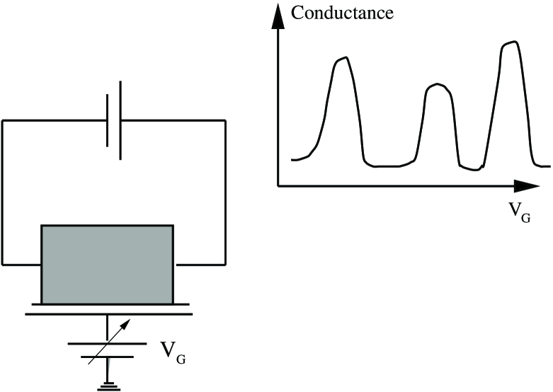
FIG. 1.: A schematic equivalent circuit of a quantum dot. Inset: The linear conductance through the dot as function of the gate voltage $V_{G}$ (schematic).

The quantum dot interferometry experiments yielded a rich set of results. Most of them came initially as a surpirse, but further analysis provided satisfactory explanations to the observed effects within single particle theories or otherwise the orthodox theory of Coulomb blockade. Certain effects, though, turned out to be more puzzling, initiating an extensive theoretical effort which is yet to prove fruitful. Some of the puzzling results even went unnoticed. I shall not attempt to present here a comprehensive review of the physics of coherence and interferometry on mesoscopic scales, nor shall I review all the relevant ( and important) literature. Instead, I provide an updated compendium of the experimental results, the dilemmas they present, and some theoretical perspectives concerning the attempts to address this physics. In fact, the present overview can be regarded as a shopping list of the present challenges in this field. Due to the limited scope of this presentation I will not address the very low temperature limit, where Kondo physics comes to play. Interesting effects are expected in that context, cf. e.g. Refs.  [12, 13, 22, 23, 24, 25]. I also note that the magnetic fields discussed here are sufficiently weak to ignore spin-related Zeeman splitting. Likewise, the systems considered are always small (or narrow) enough for the quantum Hall effect not to show up.

The outline of this paper is the following. In the next section I review some basic facts concerning AB interferometry in electronic systems, including a reference to symmetries at equilibrium (Onsager) and away from equilibrium, a brief discussion of partial coherence, and a simple demonstration of the breakdown of the Landauer formula in the presence of interaction. In Section III I discuss the phenomenon of phase locking (and a scenario for its breakdown). Section IV addresses the issue of the transmission phase correlations. In Section V we discuss the asymmetric features of the coherent AB amplitude. Finally, in Section VI I comment on the dilemmas involving the width of the Coulomb peaks as well as that of the phase lapses.

This short overview is largely based on past and present collaborations. Parts of this manuscript consist of results obtained recently in collaboration with D, E. Feldman, J. König, Y. Oreg and A. Silva.

II Aharonov-Bohm interferometry in electronic systems: some basics

Earlier on in the development of the field of Mesoscopics it became clear that AB interferometry is a most useful tool. This, of course, has to do with the fact that electrons are charged particles, and therefore the electric current is (minimally) coupled to the vector potential, A, generated by a Aharonov-Bohm flux. The vector field A influences the phase of the electron and thus affects the outcome of interference experiments. The first intriguing effect that has been noticed in that context was that while the periodicity (say, of the conductance) under the AB flux should, in principle, be $\delta\varphi=1$ [26, 27], the AB periodicity of a flux threading a (dirty) conducting cylinder was found to be $\delta\varphi={1\over 2}$ [28], a result which was confirmed in experiment [2]. While the latter periodicity was certainly in line with the Byers-Yang theorem [29], stating that equilibrium (hence linear-response) observables should be periodic under $\varphi\rightarrow\varphi+1$, the effect of period halving came as a surprise. It was later understood [30] that period halving was the result of ensemble averaging [31, 32], and that in the absence of such averaging the fundamental period should be $1$ rather than ${1\over 2}$. This indeed was found to be in line with experimental observations [3, 4]. Other exciting, interferometry-related, effects followed (such as persistent currents, orbital magnetism, flux-dependent “universal” conductance fluctuations).

Phase locking

One concept that emerged from those early studies was the phenomenon of phase locking [33, 34, 35]. To understand this effect let us first consider a two-slit experiment, depicted in Fig. 2, for which phase locking is not satisfied.

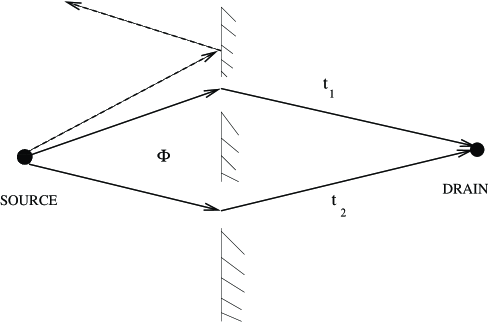
FIG. 2.: Setup for a two-slit interferometry.The dashed line represents a trajectory of an electron absorbed by a “far-gate”.

A single electron physics is assumed. The electron is emitted from the source and may be absorbed by either the drain, the source, or be “lost” (i.e. absorbed by any of the other “far gates”). This motivates later reference to this setup as open geometry. The partial amplitudes for the electron to be transmitted through slits 1 or 2 ( and eventually be absorbed by the drain) are $t_{1}$ and $t_{2}$ respectively, with

$$t_{m}=|t_{m}|\exp(i\alpha_{m})\,\,,$$ (1)

with $m=1,2$. In the presence of an AB flux the partial transmission amplitudes assume additional flux induced, gauge dependent phases,

$$\alpha_{m}\rightarrow\alpha_{m}+2\pi\varphi_{m}\,\,.$$ (2)

The relative phase of the two trajectories described by these two partial amplitudes is

$$\alpha+2\pi\varphi\equiv\alpha_{1}-\alpha_{2}+2\pi\varphi_{1}-2\pi\varphi_{2}\,\,,$$ (3)

where $\varphi\equiv\varphi_{1}-\varphi_{2}$ is the gauge invariant AB phase. The total transmission amplitude, $t_{total}=t_{1}+t_{2}$. Employing the Landauer formula [36, 33], the total transmission probability is given by

$$T_{tr}=|t_{total}|^{2}\,,$$ (4)

where $t_{total}$ is the total transmission amplitude. For our geometry it follows that

$$T_{tr}=|t_{1}|^{2}+|t_{2}|^{2}+2|t_{1}t_{2}|\cos(\alpha+2\pi\varphi)\,\,.$$ (5)

The flux sensitive interference term $2|t_{1}t_{2}|\cos(\alpha+2\pi\varphi)$ is evidently periodic in $\varphi$ (flux) with a period $1$. The asymmetry of the AB signal with respect to $\varphi=0$ is due to the appearance of the orbital phase $\alpha$. It is quite suggestive to refer to a situation where this phase shift disappears (e.g. due to some underlying symmetry, see below) as phase locking.

Partial coherence and visibility

The above expression for the total transmission probability through the double-slit configuration was derived under the conditions of full coherence. The conductance is related to the transmission probability through

$${\cal G}={e^{2}\over h}T_{tr}\,\,.$$ (6)

This relation holds for interacting systems as well. To check whether there is some degree of cohernece in the system is a relatively easy task. We only need to note that there are certain values of the flux for which the total transmission is smaller than the sum of the individual transmissions through each channel, i.e., $T_{tr}<|t_{1}|^{2}+|t_{2}|^{2}$. To assert that there is full coherence in the system is a more demanding task. Consider the expression for the total transmission, Eq.5. For $|t_{1}|\neq|t_{2}|$ the AB amplitude is smaller than the flux-averaged signal. Referring to the conductance we can write the above inequality as

$$\left\langle{\cal G}\right\rangle_{\varphi}={e^{2}\over h}(|t_{1}|^{2}+|t_{2}|^{2})>{\cal G}^{AB}=2{e^{2}\over h}|t_{1}t_{2}|>0\,\,,$$ (7)

with $\left\langle{\cal G}\right\rangle_{\varphi}$ being the flux-averaged conductance, ${\cal G}^{AB}$ is the amplitude of the (periodic) flux dependent term. It is therefore convenient to define the visibility, ${\cal V}$, of such an interferometer

$${\cal V}\equiv{\cal G}^{AB}/\left\langle{\cal G}\right\rangle_{\varphi}\,\,.$$ (8)

There could be 3 different reasons for the visibility to be smaller than one:
(i) The transmission is fully coherent, yet the transmissions through the two interferometer arms are asymmetric–one arm transmits better than the other. This is the scenario outlined above. Evidently when the two interferometer’s arms are symmetric,$|t_{1}|=|t_{2}|$, ${\cal V}=1$.
(ii) There are several transmission channels through each arm, each carrying its own orbital (and possibly AB) phase. It follows that the conditions for destructive interference are different among the different channels, and may not be satisfied simultaneously.
(iii) The transmitted electrons are coupled to other degrees of freedom [37, 38] which give rise to dephasing, setting the stage for partial coherence.

The first two scenarios are fundamentally different from the third one, as they correspond to full coherence (although the observed visibility may be smaller than unity). Indeed, full coherence implies that in principle it is possible to tune or modify the parameters of one of the arms ( “the reference arm”), and vary the flux such that full destructive interference (${\cal V}=1$) is obtained.

From the theoretical point of view there are two main approaches for incorporating dephasing processes in interferometry devices. The first one [39, 40] is phenomenological. One starts with writing down a scattering theory formalism for the problem at hand (a-la Landauer), and then adding “dephasing reservoirs” which absorb and emit electrons, usually without modifying the current. What a dephasing reservoir does is to erase any phase memory of the electrons that go through. Operationally one describes the scattering into/out of the dephasing reservoir by assigning some complex amplitude to such a process, with a phase $\theta$. Once an observable (e.g. the transmission probability through the device) is calculated, an average over $\theta$ is taken. Various generalizations of this approach are possible, e.g. the introduction of numerous, weakly coupled reservoirs along the transmission line which mimicks gradual, continuous dephasing processes [39, 40]. There are certain caveats with this procedure: The dephasing agent here is completely classical. This means that in the process of dephasing energy may be pumped into to electronic system [41]. Also, subtle quantum effects and correlations are ignored in this approach. Finally, the averaging over the phase $\theta$ does not commute with the time reversal operation; performing this averaging and then time reversing the problem may present problems with unitarity [40]. The second approach to the introduction of dephasing is microscopic One can classify the dephasing agents according to whether the coupling term in the Hamiltonian does or does not commute with the Hamiltonian of the uncoupled reservoir [42]. The physics that emerges is elaborate and not yet fully exhausted.

Two-terminal vs. multi-terminal geometries

As we have seen above, owing to the different orbital phases of the two interferometer’s arms, the AB signal is, in general, asymmetric with respect to $\varphi=0$, i.e., no phase locking takes place. This is the case for the open geometry depicted in Fig. 2, and similarly for a multiple-terminal setup, Fig. 3.

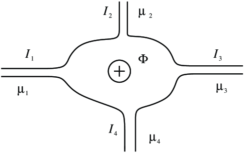
FIG. 3.: A 4-terminal AB interferometer.

In contradistinction, for a two-terminal geometry one expects phase locking to take place. We note that in such a geometry an electron leaving the source may, eventually, be either reflected back to the source or transmitted to the drain ( unlike in a multi-terminal geometry or in an open geometry where the electron may end up in one of the other “gate” terminals). The total transmission and the reflection probabilities satisfies then

$$T_{tr}+R_{ref}=1\,\,.$$ (9)

Employing Eqs. 6 and 9 the flux dependence of ${\cal G}$ can be fully deduced from $R_{ref}$, the latter obtained by taking the square modulus of the sum of the self-returning amplitudes. To accomplish this task we pretend that those amplitudes can be evaluated through an infinite set of semiclassical trajectories which we denote by $\{A_{j}^{(n)}\}$, [43]. This notation is rather symbolic, pretending that there is a countable set of relevant partial amplitudes. We classify the various partial amplitudes according to their winding number, $n$, and a running index $j$ within each class of $n$. Each of these partial amplitudes includes an orbital phase which we denote by $\alpha_{j}^{(n)}$. Furthermore, we need to assign an AB phase (which depends on the winding number only), $\varphi^{(n)}\equiv 2\pi n\varphi$. Thus

$$A_{j}^{(n)}=|A_{j}^{(n)}|\exp(i\alpha_{j}^{(n)})\exp(i\varphi^{(n)})\,\,.$$ (10)

Let $A_{j}^{(n)}$ and $A_{j}^{(-n)}$ represent two trajectories which are mutually time reversed. It follows that

$$A_{j}^{(n)}=A_{j}^{(-n)}\,\,,$$ (11)

$$\varphi^{(n)}=-\varphi^{(-n)}\,\,.$$ (12)

The reflection probability is then given by

$$R_{ref}=r\times r^{*}=\left[\sum_{j,n}A_{j}^{(n)}\right]\times\left[\sum_{j,n}A_{j}^{(n)}\right]^{*}\,\,.$$ (13)

Performing this multiplication we obtain several distinct types of terms:

(i)  ”diagonal terms”, arising from the multiplication of $A_{j}^{(n)}$ by $\left[A_{k}^{(n)}\right]^{*}$ (same winding number, $j,k$ are general). These sample specific terms amount to a flux independent contribution. In particular, the product of the partial amplitude $A_{j}^{(n)}$ with its complex conjugate rids of the (sample specific) orbital phase. Adding together the diagonal contributions of $A_{j}^{(n)}$ and $A_{j}^{(-n)}$ one obtains

$$|A_{j}^{(n)}|^{2}+|A_{j}^{(-n)*}|^{2}=2|A_{j}^{(n)}|^{2}\,\,.$$ (14)

(ii)  ”time reversed” terms, arising from the product of $A_{j}^{(n)}$ and $\left[A_{k}^{(-n)}\right]^{*}$ with $j=k$ (we will be concerned with time-reversed pairs; $j\neq k$ pairs possess sample specific orbital phases; such terms contribute to the statistical fluctuations, in much the same way as the cross-terms of type (iii)). By Eq.11 the orbital phase of a time-reversed pair cancels out, and one is left with a flux-dependent phase only. Adding up two related reversed pairs one obtains

$$A_{j}^{(n)}\times A_{j}^{(-n)*}+A_{j}^{(-n)}\times A_{j}^{(n)*}=2|A_{j}^{(n)}|^{2}\cos(4\pi n\varphi)\,\,.$$ (15)

(iii)  ”cross terms”. These are all the rest. Their magnitude is sample specific, their (orbital) phase is sample specific (hence strongly fluctuating), and in general they are flux dependent.

Detailed analysis of these terms may yield a wide spectrum of effects, basically the entire single-electron mesoscopics in a nutshell, including the effects of period-halving, negative magneto-resistance at weak magnetic fields, conductance fluctuations and more. This is beyond the scope of the present analysis. What we would like to stress here is the emergence of phase locking. This can be easily seen for the ensemble averaged problem. The terms which survive ensemble averaging are given by Eqs.(14, 15) (summation over $j$ is implied); all the other, strongly fluctuating, terms average to zero. Symmetry with respect to $\varphi=0$ is evident. Phase locking, though, is a more robust phenomenon, valid on the level of sample-specific observables. We only need to note that when performing the multiplication implied by Eq.13 we add up the following terms together: $A_{k}^{(n)}\times A_{j}^{(m)*}+A_{k}^{(n)*}\times A_{j}^{(m)}+A_{k}^{(-n)}\times A_{j}^{(-m)*}+A_{k}^{(-n)*}\times A_{j}^{(-m)*}=\\ 4|A_{j}^{(m)}A_{k}^{(n)}|\cos(\alpha_{j}^{(m)}-\alpha_{k}^{(n)})\cos((n-m)\varphi)$. Phase locking is then manifest.

Dephasing or inelastic relaxation processes may suppress the coherent transmission and reflection amplitudes (giving rise to an incoherent background)– more generally they will suppress the related single-particle Green function. It is important to notice, though, that such processes do not destroy the phase locking symmetry. A mechanism for breaking down this symmetry is discussed in Section III.

Careful examination of our analysis of the noninteracting system reveals that phase locking is satisfied within any infinitesimal energy window (we have been dealing with partial amplitudes each possessing a certain energy). In that case the validity of phase locking ( for the two-terminal geometry) is independent of the electron energy distribution function, and it extends beyond linear response. This is not the case in general, where electron-electron interactions render the notion of a “sharply defined single electron energy” inadequate. One may still prove the validity of phase locking assuming that the reservoirs at the boundaries of the system (e.g. the source and the drain) are described by a gas of non-interacting electrons . This proof, originally proposed by Büttiker [33], relies on the general Onsager relations. The fact that a finite external voltage bias can destroy phase locking has been nicely demonstrated by Bruder, Fazio and Schoeller [44].

It should be noted, though, that even away from equilibrium, when linear response does not apply, there may still be certain symmetries governing the behavior of the conductance. König and Gefen [37] noted the connection between the spatial symmetries of the underlying setup and the symmetries of the transport coefficients. In Fig. 4 we depict three different cases in which the system has a distinct spatial symmetries [37].

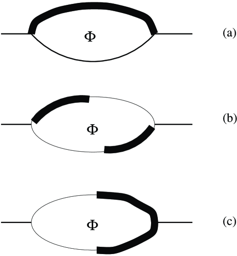
FIG. 4.: Two terminal AB interferometers with different spatial symmetry. Different lines represent different lead geometries/impurity configurations. (a) possesses mirror symmetry with respect to a vertical axis, (b) possesses a point symmetry: invariance under rotation at angle $\pi$, and (c) has a mirror symmetry with respect to a horizontal axis. The chemical potentials of the left/right reservoirs are indicated. In cases (b) and (c) phase locking is preserved even at finite bias.

The general relation for all two-terminal setups

$${\partial I(V,\varphi)\over\partial V}={\partial I(-V,-\varphi)\over\partial V}\,,$$ (16)

where $V$ is the applied bias, yields as a direct consequence the Onsager relation

$${\partial I(\varphi)\over\partial V}\bigg{|}_{V=0}={\partial I(-\varphi)\over\partial V}\bigg{|}_{V=0}$$ (17)

which leads to phase locking in linear response. Fig. 4a represents a system with a mirror symmetry with respect to its vertical axis. One clearly can reverse the direction of the bias and the sign of the AB-flux leaving the magnitude of the current unchanged. The resulting equation is

$${\partial I(V,\varphi)\over\partial V}={\partial I(-V,-\varphi)\over\partial V}$$ (18)

which coincides with Eq (16). Fig. 4b represents a point symmetry: rotation at angle $\pi$ with respect to the center. The resulting invariance is expressed through

$${\partial I(V,\varphi)\over\partial V}={\partial I(-V,\varphi)\over\partial V}\,.$$ (19)

Finally, Fig. 4c depicts a mirror symmetry with respect to a horizontal axis, leading to the equation

$${\partial I(V,\varphi)\over\partial V}={\partial I(V,-\varphi)\over\partial V}\,.$$ (20)

In the two latter cases phase locking symmetry is satisfied [37]. It either follows directly or after making use of Eq. (16). Here phase locking is a consequence of spatial symmetry. In the first case (Fig. 4a), or in the absence of any particular spatial symmetry, breaking of phase locking occurs at finite bias voltages.

Watch the Landauer formula for interacting systems

The Landauer formula provides a convenient framework to study the conductance of specific setups, relating the transmission amplitude through the system to the total transmission probability, cf. Eqs. (4,6). Things are not as simple when it comes to an interacting system. In that case any given electron interacts with other degrees of freedom ( e.g. other electrons), and its energy is not conserved– one needs to resort to a many-particle, continuous energy-channel scheme (cf. [38, 35]. The Landauer formula has indeed been generalized employing Green’s function techniques for interacting systems [45, 46, 47]. To demonstrate the failure of the naive Landauer formula, and to relate it to the concepts of partial coherence and decoherence, we present here a toy model which captures these themes [37]. Let us consider a single-level QD with level energy $\epsilon$, measured from the Fermi energy of the leads. The Hamiltonian

$$H=H_{L}+H_{R}+H_{D}+H_{T}$$ (21)

consists of $H_{r}=\sum_{k\sigma}\epsilon_{kr}a^{\dagger}_{k\sigma r}a_{k\sigma r}$ for the left and right lead, $r=L/R$. The isolated dot is described by $H_{D}=\epsilon\sum_{\sigma}n_{\sigma}+Un_{\uparrow}n_{\downarrow}$, where $n_{\sigma}=c^{\dagger}_{\sigma}c_{\sigma}$, and $H_{T}=\sum_{k\sigma r}(t_{r}a^{\dagger}_{k\sigma r}c_{\sigma}+{\rm H.c.})$ models tunneling between dot and leads (we neglect the energy dependence of the tunnel matrix elements $t_{L/R}$). Due to tunneling the dot level acquires a finite line width $\Gamma=\Gamma_{L}+\Gamma_{R}$ with $\Gamma_{L/R}=2\pi|t_{L/R}|^{2}N_{L/R}$ where $N_{L/R}$ is the density of states in the leads. The electron-electron interaction is accounted for by the charging energy $U=2E_{C}$ for double occupancy. To keep the discussion simple we choose $U=\infty$ for the QD.

As was discussed above, a contribution to the transport through a QD is identified as fully coherent if by adding a reference trajectory fully destructive interference can be achieved. Interaction of the dot electrons with an external bath (e.g. phonons) destroys coherence since interference with a reference trajectory is no longer possible: the transmitted electron has changed its state or, equivalently [48], a trace in the environment is left. One possible mechanism for suppressing coherence in interacting QDs is flipping the spin of both the transmitted electron and the QD [49].

Away from resonance, $|\epsilon|\gg k_{B}T,\Gamma$, transport is dominated by cotunneling. There are three different types of cotunneling processes (for $U=\infty$):
(i) an electron enters the QD, leading to a virtual occupancy, and then leaves it to the other side.
(ii) an electron leaves the QD, and an electron with the same spin enters.
(iii) an electron leaves the QD, and an electron with opposite spin enters.
These three processes are shown schematically in Fig. 5.

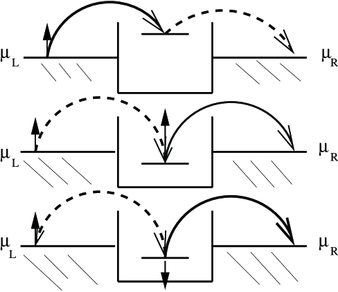
FIG. 5.: Cotunneling processes for $U=\infty$. The solid line indicates the process that happens first, the dashed line – the process that occurs afterwards. Double occupancy of the QD in the initial, intermediate, or final state is prohibited due to the infinite charging energy.

Note that double occupancy of the dot (even in a virtual state) is forbidden since we have assumed $U=\infty$. All processes are elastic in the sense that the energy of the QD has not changed between its initial and final state. In particular, process (iii) is elastic in the sense that the energy of the QD has not changed. It is incoherent, though, since the spin in the QD has flipped ( and it is therefore possible to determine that the electron under study went through the interferometer’s arm with the QD and not through the free reference arm). Such a process will then contribute to the total current but not to the flux-sensitive component thereof, independent of the specific details of the AB interferometer. The observation that energy exchange is not necessary for dephasing [50] and that the latter can take place through, e.g., a spin flip of an external degree of freedom, has been made early on [48]. In our case the electrons in the QD itself (and their spin) serve as the “dephasing bath” [38].

To evaluate the transmission probability, hence the conductance, at finite temperatures, one needs to sum over contributions from different energies. This results in

$${\cal{G}}_{\rm linear-response}\equiv{\partial I\over\partial V}\bigg{|}_{V=0}=-{e^{2}\over h}\sum_{\sigma}\int d\omega\,T_{tr}^{\sigma}(\omega)f^{\prime}(\omega)\,.$$ (22)

Here $T_{tr}^{\sigma}(\omega)$ denotes the transmission probability for an incoming electron of spin $\sigma$ and frequency $\omega$ while $f$ is the Fermi-Dirac distribution function.

The transmission through a single-level QD appearing in Eq. (22) can be obtained [45, 46, 47] from

$$T_{tr(\rm dot)}^{\sigma}(\omega)=-{2\Gamma_{L}\Gamma_{R}\over\Gamma}\,{\rm Im}\,G^{\rm ret}_{\sigma}(\omega)\,.$$ (23)

Here the dot’s Green function, given by

$$G^{\rm ret}_{\sigma}(\omega)=1/(\omega-\epsilon+i\Gamma/2)\,\,,$$ (24)

is the Fourier transform of $-i\Theta(t)\langle\left\{c_{\sigma}(t),c^{\dagger}_{\sigma}(0)\right\}\rangle$. For cotunneling, the transmission probabilities of electrons with energy $\omega$ near the Fermi level of the leads can also be obtained by calculating the transition rate in second-order perturbation theory and multiplying it with the probabilities $P_{\chi}$ to find the system in the corresponding initial state $\chi$. For an incoming electron with spin up the transmission probabilities are $P_{\chi}\Gamma_{L}\Gamma_{R}{\rm Re}[1/(\omega-\epsilon+i0^{+})^{2}]$. Here $P_{\chi}$ are the probabilities to find the system in the corresponding initial states $\chi=0,\uparrow,\downarrow$ for case (i), (ii), and (iii), respectively. Since $P_{0}+P_{\uparrow}+P_{\downarrow}=1$ and $P_{0}+P_{\sigma}=1/[1+f(\epsilon)]$ in equilibrium, we find

$$T_{tr(\rm dot)}^{\sigma}(\omega)=T_{tr(\rm dot,coh)}^{\sigma}(\omega)+T_{tr(\rm dot,incoh)}^{\sigma}(\omega)$$ (25)

with [51]

$$T_{tr(\rm dot)}^{\sigma}(\omega)={\rm Re}\,{\Gamma_{L}\Gamma_{R}\over(\omega-\epsilon+i0^{+})^{2}}\,,$$ (26)

$$T_{tr{\rm dot,con}}^{\sigma}(\omega)={T_{tr({\rm dot})}^{\sigma}(\omega)\over{1+f(\epsilon)}}\,.$$ (27)

The (evidently coherent) transmission amplitude through the QD can be defined in the following way

$$t_{(\rm dot)}^{\sigma}(\omega)=i\sqrt{\Gamma_{L}\Gamma_{R}}\,G^{\rm ret}_{\sigma}(\omega)\,.$$ (28)

We now show that Eq. (28) is not a good building block for calculating the transmission probability for interacting QDs. Employing Eq. (24) we obtain

$$t_{\sigma}^{\rm dot}(\omega)={i(P_{0}+P_{\uparrow})\sqrt{\Gamma_{L}\Gamma_{R}}\over(\omega-\epsilon+i0^{+})}\,\,,$$ (29)

from which it follows that

$$|t_{\sigma}^{\rm dot}(\omega)|^{2}={T_{tr(\rm dot)}^{\sigma}(\omega)\over[1+f(\epsilon)]^{2}}\,\,.$$ (30)

The latter equation does not yield the total transmission through the dot, nor does it represent the contribution to the transmission probability arising from the coherent part of the transmission.

We have thus demonstrated that the the presence of electron-electron interactions gives rise to spin-flip processes, i.e. to incoherent transmission channels, hence to the breakdown of Eq. (4); there is no direct physical meaning of the expression $|t_{\sigma}^{\rm dot}(\omega)|^{2}|$.

III How to break phase locking

The phenomenon of phase locking has been found [26, 27] and recognized [53] in the early days of Mesoscopics. Experiments on small normal systems (simply and multiply connected) revealed magnetoconductance which was asymmetric under reversal of the direction of the magnetic field [54]. It has been then realized theoretically that the magnetoresistance can be asymmetric in the presence of an AB flux. Following some controversy Büttiker has proposed a multi-terminal effective circuit framework which captures the essential symmetries of the problem. This approach is, in principle, generalizable to a many-body interacting system coupled to external terminals of independent electron gas.

Below we provide a brief review of Büttiker’s approach [33] (to be contrasted with the approach outlined e.g. in Section V). We then make a few comments concerning the breakdown of the two-terminal phase locking mentioned earlier. Consider the four-terminal system depicted in Fig. 3. The four terminals are connected to voltage sources (“electron reservoirs”) of chemical potentials $\mu_{i},i=1,...,4$. The reservoirs serve both as a source and a sink of carriers and energy. They possess the following properties: At zero temperature they feed the leads with carriers up to the chemical potential $\mu_{i}$. At finite temperatures they feed the leads at all energies, weighted by the Fermi-Dirac function of the corresponding temperature and chemical potential. Each carrier coming from the lead and reaching the reservoir is absorbed by the reservoir irrespectively of its phase and energy. We first assume that the terminals connecting the respective reservoirs to the system are strictly one-dimensional. This means that at each terminal there are two running states at the Fermi energy, one with positive velocity (away from the reservoir) and the other with negative velocity. At this point we ignore interactions (e.g. electron-electron) or any inelastic processes within the system (inelastic relaxation and dephasing processes take place in the reservoirs). The electrons are scattered elastically in the system. We next assign scattering probabilities $\{T_{ij}(\varphi)\}$ for carriers outgoing from terminal $j$ to be transmitted into terminal $i$; we also use the notation $\{R_{ii}(\varphi)\}$ to denote reflection probabilities from $i$ to $i$. It is clear that

$$T_{ij}(\varphi)=T_{ji}(-\varphi)\,\,,$$ (31)

$$R_{ii}(\varphi)=R_{ii}(\varphi)\,.$$ (32)

These relations can be easily verified employing equations akin to Eqs. (10) and (13). As we are interested in linear response, the differences among the various $\{\mu_{i}\}$ are small, rendering the transmission and reflection probabilities $\{T_{ij}(\varphi)\}$ and $\{R_{ii}(\varphi)\}$ energy independent.

Straightforward algebra leads to the following expression for the current in the $i$-th lead

$$I_{i}={e\over h}\left[(1-R_{ii})\mu_{i}-\sum_{j\neq i}T_{ij}\mu_{j}\right]\,.$$ (33)

Particle conservation, $R_{ii}+\sum_{j\neq i}T_{ij}=1$, implies that Eq. (33) is independent of the choice of the reference potential ($\mu=0$).

Let us first consider an arrangement [33, 55] where the currents satisfy $I_{1}=-I_{3}$ and $I_{2}=-I_{4}$. Inserting into Eq. (33) we obtain

$$I_{1}=\chi_{11}(V_{1}-V_{3})-\chi_{12}(V_{2}-V_{4})\,,$$ (34)

$$I_{2}=-\chi_{21}(V_{1}-V_{3})+\chi_{22}(V_{2}-V_{4})\,,$$ (35)

where $V_{i}=\mu_{i}/e$. Büttiker then found the following expressions for the generalized conductances of Eq. (34):

$$\chi_{11}={e^{2}\over h}\left[(1-R_{11})S-(T_{14}+T_{12})(T_{14}+T_{21})\right]/S\,,$$ (36)

$$\chi_{12}={e^{2}\over h}(T_{12}T_{34}-T_{14}T_{32})/S\,,$$ (37)

$$\chi_{21}={e^{2}\over h}(T_{21}T_{43}-T_{23}T_{41})/S\,,$$ (38)

$$\chi_{22}={e^{2}\over h}\left[(1-R_{22})S-(T_{21}+T_{23})(T_{32}+T_{12})\right]/S\,,$$ (39)

where

$$S=T_{12}+T_{14}+T_{32}+T_{34}=T_{21}+T_{41}+T_{23}+T_{43}\,.$$ (40)

The last equality is obtained by connecting terminals $1$ and $3$ together, and similarly terminals $2$ and $4$. One then obtains a two-terminal geometry, for which it is clear that the transmission $(1,3)\rightarrow(2,4)$ is equal to the transmission in the reverse direction, $(2,4)\rightarrow(1,3)$. Employing Eq. (31) one obtains

$$\chi_{11}(\varphi)=\chi_{11}(-\varphi)\,,$$ (41)

$$\chi_{22}(\varphi)=\chi_{22}(-\varphi)\,,$$ (42)

$$\chi_{12}(\varphi)=\chi_{21}(-\varphi)\,.$$ (43)

Eq. (41) establishes the Onsager relation for this circuit.

We next select the current source and drain to be terminals $1$ and $3$ respectively, and assume that $2$ and $4$ are potentiometer terminals, implying that the voltages $V_{2},V_{4}$ are measures under the condition $I_{2}=I_{4}=0$. One can now define a four-terminal conductance

$${\cal G}_{13,24}={1\over 2}{{I_{1}-I_{3}}\over{V_{2}-V_{4}}}\,.$$ (44)

(We have used $I_{1}={1\over 2}(I_{1}-I_{3})$ to cast ${\cal G}_{13,24}$ in a symmetric form). From Eqs. (34), (36) and (41) one obtains

$${\cal G}_{13,24}={{\chi_{11}\chi_{22}-\chi_{12}\chi_{21}}\over{\chi_{21}}}\,.$$ (45)

Since $\chi_{21}$ is not symmetric in $\varphi$, ${\cal G}_{13,24}$ turns out to be asymmetric as well (although the Onsager relations are clearly satisfied [33]).

We now face the following paradox. Consider a two-terminal AB interferometer. Let us now embed a “conducting island” in each of the interferometer’s arms. Since this is a two-terminal setup, we expect phase-locking to hold. On the other hand, once we make the embedded islands sufficiently large, we may expect that eventually they would represent electron reservoirs (as if we have added two extra terminals to the circuit), leading perhaps to the breakdown of phase locking? If this is indeed the case – what is the characteristic island size where this breakdown can be observed? We first call attention to the fact that, as was discussed above, the mere introduction of inelastic or phase breaking processes cannot lead to the breakdown of phase locking. To address these questions we note [56] that in the context of four- ( or multi-) terminal geometries it is possible to define other quantities whose dimension is conductance. One quantity of interest is

$${\cal G}_{13,13}={1\over 2}{{I_{1}-I_{3}}\over{V_{1}-V_{3}}}\,.$$ (46)

Similarly we define

$${\cal G}_{13,13}^{\prime}={{I_{1}}\over{V_{1}-V_{3}}}\,,$$ (47)

and

$${\cal G}_{13,13}^{\prime\prime}=-{{I_{3}}\over{V_{1}-V_{3}}}\,.$$ (48)

It is clear that as long as $I_{2}=I_{4}=0$, ${\cal G}_{13,13}={\cal G}_{13,13}^{\prime}={\cal G}_{13,13}^{\prime\prime}$, and phase locking follows immediately (we note that in this case the only efffect of the extra terminals is to modify the effective elastic and inelastic scattering rate in the two-terminal interferometer).

We now modify $V_{i}$ slightly into $V^{\prime}_{i}=V_{i}+\delta V_{i},i=2,4$, such that there is small current flowing out of terminal $2$ while the current through terminal $4$ is still zero. Then $I_{3}=-(I_{1}+I_{2})\neq-I_{1}$. and the definition of conductance $G_{13,13}$ becomes ambiguous: $G_{13,13}=1/2(I_{1}-I_{3})/(V_{1}-V_{3})\neq G_{13,13}^{\prime}=I_{1}/(V_{1}-V_{3})\neq G_{13,13}^{\prime\prime}=-I_{3}/(V_{1}-V_{3})$. A simple calculation yields

$$G_{13,13}=(\chi_{11}\chi_{22}-\chi_{12}\chi_{21})/\chi_{22}-\chi_{12}I_{2}/[\chi_{22}(V_{1}-V_{3})]=$$ (49)

$$A(\Phi)+B(\Phi)I_{2}/(V_{1}-V_{3})\,\,.$$ (50)

By Eq. (41) the first term in Eq. (49) is invariant under the transformation $\Phi\rightarrow-\Phi$. However, the second term which is nonzero in the presence of $I_{2}$ is not invariant under this transformation. The condition for the extremum of the conductance ( as function of the flux) is $A^{\prime}(\Phi)+I_{2}B^{\prime}(\Phi)/(V_{1}-V_{3})=0$. Since $A^{\prime}(0)=0$, we estimate the derivative $A^{\prime}(\Phi)$ as $A^{\prime\prime}(0)\Phi$ at small $\Phi$. For small $I_{2}$ this gives for the extremum $\Phi_{\rm extr}=-I_{2}B^{\prime}(0)/[A^{\prime\prime}(0)(V_{1}-V_{3})]$. The flux $\Phi_{\rm extr}$ is nothing else but $-\alpha\Phi_{0}/2\pi$, where $\alpha$ is the orbital phase introduced above.

The above observations can be used for a systematic study of a ”gradual breaking” of phase locking, characteristic of two-terminal geometries. A study of the breakdown of phase locking in connection the loss of unitarity may also be found in Ref. [57].

We finally note that, in a sense, phase-locking may be broken even in a two-terminal geometry if the applied magnetic flux is not purely of a Aharonov-Bohm type. Once the magnetic flux penetrates into the arms, different semi-classical trajectories of the electron’s path will enclose different amount of flux, and the strict periodicity in $\Phi$ is broken. It follows that while ${\cal G}(\varphi)={\cal G}(-\varphi)$ still holds, the relation ${\cal G}(\varphi=n+\delta)={\cal G}(\varphi=n-\delta)$ is broken.

IV The Dilemma of the transmission phase

The discussion in Section (II) shows that in general there is a coherent component of the electron transmitted through a QD. It is therefore legitimate to ask what the phase associated with the transmitted amplitude is. This is a particularly interesting issue since the role of e-e interactions in a low (zero) dimensional system, i.e. a QD, is expected to be enhanced. This question has indeed been taken up by experimentalists. It is clear that to obtain information about quantum phase one needs to resort to interferometry experiments. Typically the setup of such experiments consists of a 2DEG AB interferometer. The latter includes a $G_{a}A_{s}/AlG_{a}A_{s}$ heterostructure QD embedded in one of its arms, and a free arm which serves as reference. The QD is manipulated by varying its gate voltage. In addition one controls the AB flux, the strength of the dot-lead coupling and the temperature. The first measurement (Ref.[10]), employing a two-terminal setup, produced only limited information, having to do with the phenomenon of phase locking. Later open-geometry experiments (Ref.[11]) yielded the flux dependent component of the conductance of an AB interferometer ${\cal G}^{AB}(\varphi)$, as function of the parameter $V_{G}$ (the gate voltage). This can be written as

$${\cal G}^{AB}(\varphi,V_{G})=A(V_{G})g^{AB}(2\pi\varphi+\alpha(V_{G})),$$ (51)

where $g^{AB}$ is a periodic function of $\varphi$. The prefactor $A(V_{G})$ is expected to be large (small) for values of $V_{G}$ that correspond to Coulomb peaks (conductance valleys). Recalling Eq. (5) for non-interacting electrons (in the double-slit geometry alluded to above only the first harmonic in the AB flux appears), it is tempting to draw an analogy between $\alpha(V_{G})$ of Eq. (4) and the orbital phase of Eq. (3). If the orbital part of the transmission phase through the reference arm, $\alpha_{1}$, is insensitive to the gate voltage, one may be motivated to refer to $\alpha(V_{G})$ (up to the constant $\alpha_{1}$), as the transmission phase through the QD. In doing so we stress again that for interacting electrons the transmission probability is not given by the square of the transmission amplitude, Eq. (4).

Thus, in a strict sense, the naive interpretation of $\alpha(V_{G})$ outlined above is wrong. One, however, notes that the flux dependent part of the transmission probability is given by [37]

$$T_{2}^{AB}(\omega)=2\sqrt{\Gamma_{L}\Gamma_{R}}|t^{\text{ref}}|\cos(2\pi\varphi)\text{Re}G^{\text{ret}}(\omega)$$ (52)

for a two-terminal geometry and

$$T^{AB}_{\text{open}}(\omega)=2\sqrt{\Gamma_{L}\Gamma_{R}}|t^{\text{ref}}|\text{Re}|e^{-i(2\pi\varphi+\alpha)}G^{\text{ret}}(\omega)|$$ (53)

for an open geometry. Here $\Gamma_{L},\Gamma_{R}$ are the dot-lead couplings (on the left and right side respectively); $t^{\text{ref}}$ is the transmission amplitude through the reference arm alone); $G^{\text{ref}}$ is the retarded Green function of the coupled dot and $\omega$ is the incident’s electron energy measured from the Fermi energy. The expression for $T_{\text{open}}^{AB}(\omega)$ is analogous to the interference term in Eq. (5) (roughly speaking, the left-right Green function through the dot replaces the transmission amplitude through the dot, $t_{2}$). It is this fact that justifies referring to $\alpha(V_{G})$ as the transmission phase.

Typical parameters for the interferometry circuit are $U\approx 500\mu EV,\ k_{B}T\approx 10\mu eV$ and $\varepsilon_{F}\approx 10meV$. The number of electrons in the dot $N_{el}\approx 200-500$. The mean level spacing $\Delta\approx\varepsilon_{F}/N_{el}\approx 50-150\mu eV$, hence $T\leq\Delta$. The dot-lead coupling $\Gamma\approx 1\mu eV<T$. This set of parameters refers to the large QD experiments of Refs.[10] and [11]. In recent experiments [12], [13] smaller QDs were used in order to facilitate probing of Kondo physics. Our present review does not include discussion of this limit.

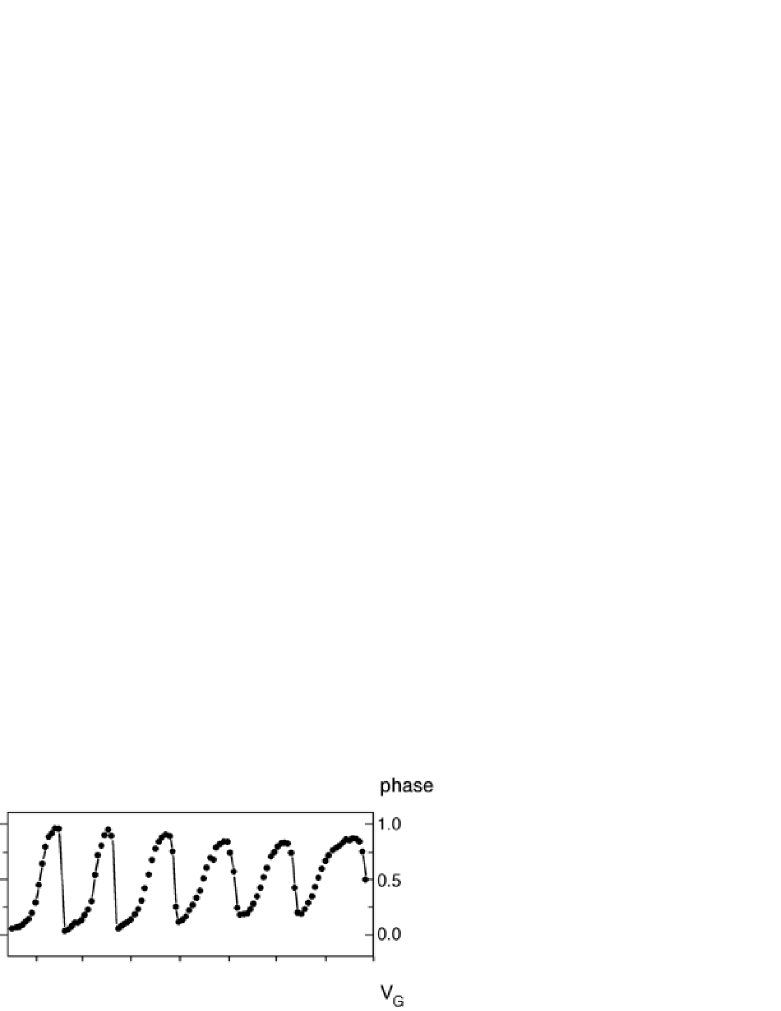
FIG. 6.: The evolution of the transmission phase $\alpha(V_{G})$ from Ref. [11]

The evolution of $\alpha(V_{G})$ is shown in Fig. 6 as function of the gate voltage. The latter is swept across consecutive Coulomb resonances. The phase $\alpha$ increases by $\pi$ as $V_{G}$ is swept across a Coulomb peak [deviations from $\pi$ are, presumably, due to the fact that the induced resonances are not entirely independent: the ratio $\Delta/\Gamma$ is not sufficiently large]. This comes as no surprise and can easily be accounted for if one represents each individual resonance by a Breit-Wigner Lorentzian. The width of the $\pi$-step in $\alpha$ at resonance is of the order of the resonance width. At low temperatures the latter is denoted by $\tilde{\Gamma}$ (in Section VI we comment on the differences between the bare (golden rule) level width $\Gamma$ and $\tilde{\Gamma}$), and remains so as long as $k_{3}T<<\tilde{\Gamma}$. In the conductance valley (i.e., between consecutive Coulomb peaks), the phase appears to drop rather sharply by $\pi$, rendering the phase evolution over a single period (in $V_{G}$) of Coulomb oscillations 0. These valley-to-valley correlations in the transmission phase have been observed repeatedly in a number of measurements, spanning up to 12 consecutive peaks in a single measurements.

This remarkable result soon attracted the attention of theorists, stimulating a large number of papers attempting to explain this phenomenon. I shall not try to present a comprehensive overview of these works. Instead I will mention the main approaches and state to what extent the problem still remains open.

The first point to note in this context is that these transmission phase correlations cannot be accounted for by independent electron theories [58]. Indeed, for a non-interacting “one-dimensional QD” (a segment of a one-dimensional wire of length $L$ bounded by two potential barriers, whose respective transmission and reflection amplitudes from left (right) are $t_{1},r_{1},t_{2},r_{2}$ $(t^{\prime}_{1},r^{\prime}_{1},t^{\prime}_{2},2^{\prime}_{2})$) the transmission amplitude for an incoming electron of wave-number $k$ is

$$t_{1dQD}=\frac{t_{1}t_{2}e^{ikL}}{1-r^{\prime}_{1}r_{2}e^{i2kL}}.$$ (54)

It is easy to determine that as one varies the incoming electron’s energy (or, alternatively, the base potential of the one-dimensional QD) the phase of $t$ varies by $\pi$ across a transmission resonance (i.e., across the energy of a quasi-bound state). This, however, is not accompanied by any phase lapse between resonances. The overall change of the transmission phase over a single period (as we increase the energy of the incoming electrons from, say, just below the $n$-th resonance to just below the $(n+1)$-st resonance) is therefore $\pi$, in stark contradistinction with the experimental data. This change-by-$\pi$-per-period is intimately connected with the fact that the sign $(p(n))$ of the product of the coupling matrix elements of the $n$-th wave function of the dot to the left and to the right leads alternates with $n$ [58] (We consider here a system which possesses time reversal symmetry (e.g., no magnetic field)). The single particle wave functions of the uncoupled dot can thus be chosen to be real; by an appropriate gauge the dot-lead matrix elements can also be made real. The sign of the latter [58], [59] is that of the derivative of the component of the wave function normal to the dot-lead interface, cf. Ref [60]. For a two- or three-dimensional non-interacting dots $p(n)$ is geometry dependent and, in general, does not show any robust $n$-independence to account for the experimental data. Furthermore, for chaotically shaped or diffusively disordered QDs, the signs of the derivative of consecutive single-particle wave functions (near the lead), hence $p(n)$, are (to leading order) uncorrelated (unlike spectral properties). It is thus evident that we need to go beyond the independent particle framework.

Some of the early attempts to resolve the transmission-phase correlation effect [61] (see also [24]) relied on the Friedel sum rule [62, 63] which provides for a relation between phase and charge. One needs, though, to call attention to the fact that the Friedel sum rule deals with the scattering matrix (rather than the transmission matrix). It relates the total charge displaced in the field of a fixed impurity (e.g., the charge added to a quantum dot) to the scattering by that impurity of a free electron at the Fermi momentum $k_{F}$. The number of displaced electrons, $N_{D}$, is given by

$$N_{D}=\frac{1}{\pi}\sum_{l,m_{l},m_{s}}\delta_{l,m_{l},m_{s}},$$ (55)

where the sum runs over the scattering phases $\delta$ with $(l,m_{l}),m_{s}$ being the angular momentum and the spin quantum numbers. More generally one can write

$$N_{D}=\frac{1}{2\pi i}T_{r}\ln S(\mu)$$ (56)

where $S(\mu)$ is the scattering matrix for single-particle-like excitations at the chemical potential $\mu$. Consider for a moment the scattering of non-interacting electrons in one-dimension [64]. (We assume that the scattering is spin independent, hence suppress the spin index). This two-channel problem is described in terms of a $2\times 2$ matrix

$$S=\left(\matrix{r&t^{\prime}\cr t&r^{\prime}\cr}\right)$$ (57)

whose eigenvalues are $e^{i\theta_{l}},l=1,2$ (primed quantities refer to reflection and transmission coefficients for electrons impinging on the scatterer from the right). The one-dimensional version of the Friedel sum rule asserts that [64]

$$n(\varepsilon)=\frac{1}{2\pi}\frac{\delta(\theta_{1}+\theta_{2})}{\delta\varepsilon}\,\,,$$ (58)

where $n(\varepsilon)$ is the density of states contained in the scatterer. It can also be shown that for the 1d case the transmission amplitude, parameterized as $t=|t|e^{i\alpha}$, leads to the relation

$$\frac{\theta_{1}+\theta_{2}}{2}=\alpha+\frac{\pi}{2}\qquad(1d)\,\,.$$ (59)

Therefore, specifically for the 1d case, the Friedel sum rule can be expressed, e.g., through Eq. (59), with the transmission phase $\alpha$ replacing the scattering phases. This, however, is not a general theorem concerning the transmission phase. Furthermore, there is no reason why the total charge accumulated at the scatterer (the QD and the leads near it) over a Coulomb period should be an integer (let alone 0, as is required if the total charge of the scattering phase were to be 0).

The theoretical effort addressing the correlations in the transmission phase could be divided, in large part, into two approaches.

The first school of thought maintains that there are one or few dot levels which are particularly strongly coupled to the leads. Such a strongly coupled level will dominate a number of consecutive transmission peaks. This would imply that successive resonances are dominated by the same tunneling matrix elements. In other words, it is practically the same level which keeps repeating at consecutive resonances, leading to transmission phase correlations over successive Coulomb periods.

As a specific example one may invoke a model QD whose Hamiltonian is made primarily of an integrable part (its eigenstates are products of longitudinal and transverse modes). The subset of states possessing high longitudinal quantum numbers defines the strongly coupled levels. The location of the gates is chosen in such a way that the energies $\{E^{0}_{\alpha}\}$ of the strongly coupled states, $\{F_{\alpha}\}$, are weakly dependent on the gate voltage. We now switch on a small non-integrable term of the potential. This leads to avoided level crossing (of the original, ”bare” levels), as function of $V_{G}$. As is demonstrated in Fig.(7) an actual single-particle level, $\psi_{n}$, (plotted as function of $V_{G}$), is now made piecewise of strongly (flat) and weakly (steep) coupled bare states (F’s and S’s). In particular, a given $F_{\alpha}$ will be equal to $\psi_{n}$ for a certain window of $V_{G}$, to $\psi_{n+}$ for the next interval of $V_{G}$ etc. It so happens that as the levels $n,n+1,n+2,\ldots$ cross successively into the Fermi sea, what used to be the (bare) level $F_{\alpha}$ will keep “floating” over the Fermi level, dominating successive Coulomb resonances.

While this picture [66, 67] provides a correlation-generating mechanism, it has a couple of nagging weaknesses. Firstly, for the level $F_{\alpha}$ to keep ”hovering” just above the Fermi energy, an (approximate) commensurability condition is required between intervals (in $V_{G}$) of consecutive avoided crossings and intervals (in $V_{G}$) over which an additional electron is added to the QD (Coulomb period). This imposes rather stringent constraints on the geometry and the confining potential. Secondly, this picture assumes that the dot’s levels (varying as function of $V_{G}$) are made piecewise of the original bare levels. The latter, other than at value of $V_{G}$ that correspond to avoided crossing, do not mix, implying that the effect of the non-integrable term in the Hamiltonian is weak. Some of the QDs studied in the experiments of the Weizmann group might be indeed almost integrable, and the above approach may be suited to describe the pertinent physics. On the whole, though, this approach lacks the flavor of being generic, i.e., pertaining to chaotic or diffusive QDs where level mixing is strong. As for the first reservation mentioned above the good news is that both finite temperature [65] or quantum [68] fluctuations render the “hovering effect” (i.e., the dominance of a single level $S_{\alpha}$ over a number of consecutive Coulomb peaks) more robust.

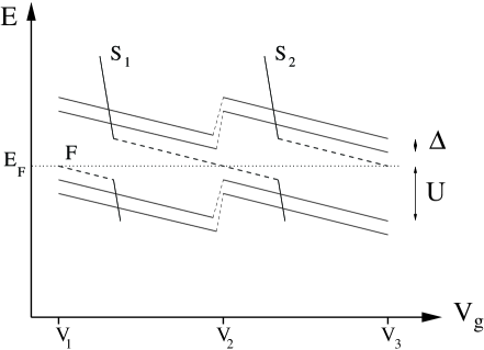
FIG. 7.: Avoided crossings with the steep bare levels $S_{1}$ and $S_{2}$ cause the flat- and strongly coupled- bare level $F$ (dashed) to stay close to the Fermi energy $\varepsilon_{F}$. Resonances dominated by this level occur at gate voltages $V_{1},V_{2},V_{3}$. There is a gap of magnitude $U$ between the last occupied and the first empty level. From Ref. [65]

The second school of thought addressing the phase correlation effect takes the opposite point of view. Rather than a single, particularly strongly coupled level, dominating the transmission phase over a wide interval of $V_{G}$, here we rely on the fact that the coherent transmission in the “conductance valley” (i.e., between Coulomb peaks) is mostly due to the process of elastic cotunneling. A parametrically large number of levels (of order $U/\Delta$) participate, each making a small (in magnitude) and random (in magnitude and phase) contribution to the transmission amplitude through the QD. Shifting the gate voltage to the next valley, these are almost the very same dot’s levels that contribute, leading (with a high probability) to the same phase of the transmission amplitude. This is the mechanism behind the valley-to-valley correlations. Detailed analysis of the phase evolution following this picture is presented in Ref. [69]

V Asymmetry of the interference signal

Let us consider transport through the QD away from resonance. At temperatures higher than the Kondo temperature this is dominated by cotunneling (second order in $\Gamma$). From the discussion of Section II [37] it turns out that such cotunneling effects give rise to an asymmetry of the AB amplitude measured on either side of a Coulomb conductance peak. To see this consider, for example, the two level QD modelled by the Hamiltonian of Eq. 21. We tune the gate voltage such that the Fermi energy is a distance $\epsilon(\ll U)$ above (or below) the Coulomb resonance separating the $N_{el}=0$ from the $N_{el}=1$ valley ($N_{el}$ is the mean number of electrons on the dot). For $\epsilon\gg\Gamma,k_{B}T$ the dominating cotunneling process on the $N_{el}=0$ side of the conductance peak is the first (coherent) process depicted in Fig. 5, while on the $N_{el}=1$ side cotunneling is dominated by the other two processes depicted in Fig. 5. These two processes are of equal probability $\sim\Gamma_{L}\Gamma_{R}{\rm Re}[1/(\omega-\epsilon+i0^{+})^{2}]$. Only one of them is coherent (the second in that figure) while the other contributes to the current through the QD but not to the flux dependent conductance ${\cal G}^{AB}(\varphi)$. If we compare two values of $V_{G}$ on either side of the conductance peak for which the flux-averaged conductance is the same, we expect greater visibility on the $N_{el}=0$ side, hence (cf. Eq. 8) a larger AB amplitude on that side. This would imply that the the AB amplitude is asymmetric with respect to the total conductance (as a function of $V_{G}$).

Our detailed analysis [37] reveals that this asymmetry exists both near resonance (going to first order in $\Gamma$) and in second order. Considering an AB interferometer with a QD in one of the arms, and tuning the transmission of the reference arms to $|t_{\rm ref}|=\sqrt{\Gamma_{L}\Gamma_{R}}/|\epsilon|$ (to maximize the visibility) one finds for the total conductance

$${\partial I^{\rm tot}\over\partial V}\bigg{|}_{V=0}={4e^{2}\over h}{\Gamma_{L}\Gamma_{R}\over\epsilon^{2}}\left[1-{\epsilon\over|\epsilon|}\cos\varphi\right]$$ (60)

for the noninteracting case ($U=0$) and

$${\partial I^{\rm tot}\over\partial V}\bigg{|}_{V=0}=4{e^{2}\over h}{\Gamma_{L}\Gamma_{R}\over\epsilon^{2}}\left[1-{\epsilon\over|\epsilon|}{\cos\varphi\over 1+f(\epsilon)}\right]$$ (61)

for $U=\infty$. This shows that cotunneling in the noninteracting case is fully coherent (we can tune both $t_{\rm ref}$ and $\varphi$ such that the total transmission probability – hence the conductance– vanishes. In the interacting case spin-flip processes are present which spoil coherence. This is described by the asymmetry factor $1/[1+f(\epsilon)]$, in accordance with our intuitive picture (in the above expressions the conductance peak is at $\epsilon=0$.)

The above considerations can be generalized for a multilevel QD. The asymmetry factor can be used to obtain information concerning the total spin of the QD in a parameter regime away from the Kondo limit.

In Fig.8 and Fig.9 we present unpublished data concerning the dependence on gate voltage of both the total conductance through the AB interferometer and and magnitude of the flux-modulated amplitude. The curves presented in Fig.8 agree qualitatively with the above discussion: for the small QD data it is possible to identify and distinguish between Coulomb blockade valleys (where the total number of electrons is presumably even) and Kondo valleys ( odd number). The latter can be identified through the very low temperature behavior of the conductance, not shown here [12, 13]. The theoretical prediction is that the peaks of the AB curve are shifted asymmetrically ( with respect to the conductance peaks) away from the Kondo valleys, which is indeed suggested by Fig.8. Surprisingly enough this seems not to be the case for the large dot curve, Fig.9, where the peaks of the AB amplitude appear to be all shifted to the right of the conductance peaks.

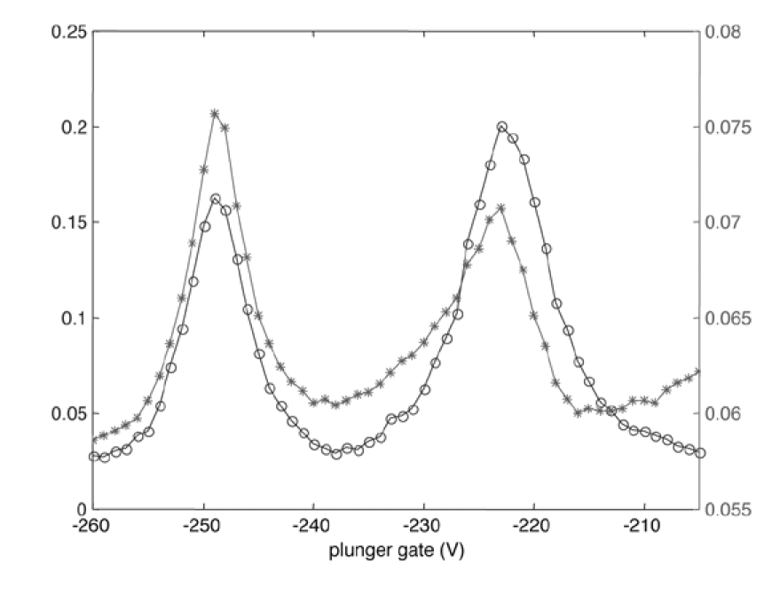
FIG. 8.: Total conductance(circles) and the AB amplitude (dots) as function of $V_{G}$ for a single (small) QD interferometer. Data are courtesy of Yang Ji and M. Heiblum

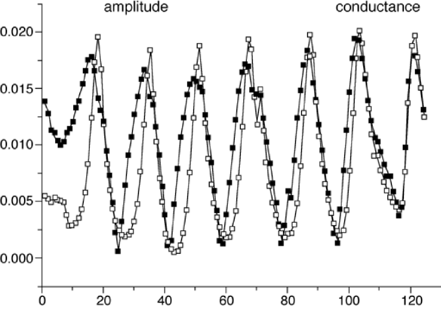
FIG. 9.: Total conductance (grey) and AB amplitude (black) as function of $V_{G}$ for a large QD interferometer. Data are courtesy of R. Schuster, Yang Ji and M. Heiblum

One might note the shape of the conductance ( and the AB) peaks is asymmetric as well. It was proposed that this is a manifestation of the Fano resonance effect, cf. Refs. [70, 71, 72, 73, 24, 74].

VI On the Width of the Resonance and the Phase Lapses

The evolution of the transmission phase discussed above presents us with further dilemmas which have been pretty much ignored till now. These concern with the widths of both the phase change by $\pi$ at the Coulomb peaks and the phase change (again by $\pi$) at the phase lapses. These widths are measured on the scale of (the change of) the gate voltage $V_{G}$. The issue is yet far from being resolved. Here we shall present the problems and add a few comments.

Let us first consider the range of $V_{G}$ (near resonance) over which the phase change by $\pi$ takes place. This is also the width of the Coulomb peak. We first consider “metallic dots”, meaning that $k_{B}T>\Delta$. It is commonly accepted that (at least for a multichannel dot-level coupling) the physics of the Coulomb peaks is a function of the dimensionless dot-level conductance, $g_{DL}$. We will assume that the couplings of the $QD$ to the left and to the right leads are of comparable strengths. We also note that $g_{DL}\sim\frac{\Gamma}{\Delta}$, where $\Gamma$ is the (bare) golden-rule width of a dot’s level. One should be careful distinguishing $\Gamma$ from $\tilde{\Gamma}$, the latter being the width of the Coulomb peak. In the weak coupling limit [16] $\tilde{\Gamma}\sim\max(\Gamma,k_{B}T)$ (for a metallic dot $\tilde{\Gamma}$ is dominated by $k_{B}T$ in this limit)[75]. To get the flavor of the dilemma involved, let us now replace the actual Coulomb peaks by a periodic (in $V_{G}$) sequence of identical Lorentzians

$$\frac{d(\text{conductance})}{d(\text{energy})}=\frac{e^{2}}{\pi h}\sum_{m}\frac{\tilde{\Gamma}}{(V_{G}-mU)^{2}+\tilde{\Gamma}^{2}}$$ (62)

The Fourier transform of the above expression (with respect to the gate voltage) is

$$\frac{e^{2}}{2\pi h}\sum_{n}e^{-\frac{2\pi n\tilde{\Gamma}}{U}}e^{i2\pi nV_{G}/U}.$$ (63)

This behavior is characteristic of mesoscopic systems. For observables which are periodic in some parameter, higher harmonics are suppressed faster (as function of width, inelastic rate, dephasing rate etc.)

Turning now our attention to the strong coupling limit one expects that the periodic modulation (of the conductance, the derivative of the particle number etc.) is all but suppressed. Only exponentially small modulation survives (of order $e^{-\frac{\pi^{2}}{8}g_{DL}}$) [76, 77]. In the language of the above Fourier expansion this amounts to the first harmonic being

$$e^{-\frac{\pi}{4}\frac{\Gamma}{\Delta}}e^{i2\pi nV_{G}/U},$$ (64)

(higher harmonics will be suppressed even further) [78]. The fact that the (exponentially small) first harmonic dominates implies that the width of the (exponentially small) “Coulomb peak” is $\sim U$. Comparing Eqs. (63) and (64) (at $\Gamma/\Delta\sim 1$) reveals that in the vicinity of the weak-to-strong-coupling crossover, $\tilde{\Gamma}$ changes dramatically from $\tilde{\Gamma}\sim k_{B}T$ (or $\Gamma$) to $\tilde{\Gamma}\sim U$ over a rather small interval of $V_{G}$. We also note that Eqs. (63) and (64) cannot be reconciled within a single parameter scaling theory [79]. We stress that at this point our considerations are rather qualitative. We expect a similar fast crossover of $\tilde{\Gamma}$ (from the weak to the strong coupling limit) with other quantities as well, e.g. $d\langle N_{el}\rangle/d_{V_{G}}$, where $\langle N_{el}\rangle$ is the expectation value of the number of electrons on the QD. We also expect a fast crossover of $\tilde{\Gamma}$ in the discrete level limit ($k_{B}T<\Delta$) as well.

Let us now turn our attention to the width of the phase lapses that occur in the “Coulomb valleys”, between Coulomb peaks. As has been discussed earlier, a universally accepted theory for such phase lapses is not yet available. Here we focus on another interesting observation – it appears that the experimentally observed typical width of these phase lapses, $\Gamma_{PL}$, is significantly smaller than that of the Coulomb peak, $\tilde{\Gamma}$. Presently this is a qualitative observation, yet to be backed up by a detailed study.

It is indeed a challenge to find a mechanism which provides for $\Gamma_{PL}$ which is parametrically smaller that $\tilde{\Gamma}$. In order to develop a feel as to what the difficulty is let us consider a toy model which exhibits a phase lapse. This is a spinless two-level QD coupled to two leads with the Hamiltonian (cf. Eq. 21)

$$H=\sum\epsilon_{k,\alpha}\;c^{\dagger}_{k,\alpha}c_{k,\alpha}+\sum_{j}\epsilon_{j}d^{\dagger}_{j}d_{j}+\\ +\sum_{k,\alpha,j}\left[V_{\alpha,j}c^{\dagger}_{k,\alpha}d_{j}+h.c\right],$$ (65)

Here the operators $c_{k,\alpha}$ refer to the electronic states in the leads ($i=L,R$) and the operators $d_{1},d_{2}$ are associated with the QD states. We note that each of the dot’s level will acquire a width $\Gamma$ due to its coupling to the leads (this width may be further renormalized due to higher order dot-lead tunnelling processes, c.f. Ref. [80]). We have intentionally chosen all dot-lead matrix elements to have the same sign. It can be shown that this indeed leads to a phase lapse [81, 82]. Moreover, the original analysis, treating the tunnelling into/from each dot level independently, results in the phase lapse having a width of $\Gamma=2\pi V^{2}\rho$ ($\rho$ is the density of status in the leads). However, our recent analysis of Eq. 65 [83] shows that the tunnelling-induced coupling between the QD’s levels must not be neglected. Since the toy model at hand is of non-interacting electrons, its analysis is straightforward. The single electron Greens function is given by

$$G(w)=\left[w-\tilde{\mathcal{H}}\right]^{-1}$$ (66)

where, in terms of the variables $\tilde{\varepsilon}=-(\varepsilon_{1}+\varepsilon_{2})/2$ and $\delta_{G}=(\varepsilon_{1}-\varepsilon_{2})/2$ the effective Hamiltonian of the QD (in the Hilbert space of levels 1,2) is

$$\tilde{\mathcal{H}}=\left(\matrix{-\tilde{\varepsilon}+\delta\varepsilon-i\Gamma&-i\Gamma\cr-i\Gamma&-\tilde{\varepsilon}-\delta\varepsilon-i\Gamma\cr}\right).$$ (67)

One can readily find

$$G(w)=\frac{1}{D(w)}\left(\matrix{w+\tilde{\varepsilon}+\delta\varepsilon+i\Gamma&-i\Gamma\cr-i\Gamma&w+\tilde{\varepsilon}-\delta\varepsilon+i\Gamma\cr}\right),$$ (68)

when the determinant $D(w)=(w+\tilde{\varepsilon})^{2}-(\delta\varepsilon)^{2}+2i\Gamma(w+\tilde{\varepsilon})$. The transmission amplitude from left to right can be written as

$$t(w)=\Gamma\sum_{i,j=1,2}G_{i,j}(w)=\frac{2\Gamma}{D(w)}(w+\tilde{\varepsilon}).$$ (69)

Varying the gate voltage amounts to varying $\tilde{\varepsilon}$ (leaving all other parameters unchanged). It is clear from Eq. 69 that one can tune the gate voltage (hence $\tilde{\varepsilon}$) to obtain an exact zero of the transmission amplitude between two peaks. This occurs for $w=-\tilde{\varepsilon}$. Sweeping $V_{G}$ around this point results in a sign change of $t(w)$, hence a zero-width phase lapse [83]. This phase lapse acquires a finite width at finite temperatures, or when the hopping matrix elements assume non-trivial relative phases. The above discussion (presented here for a non-interacting QD) demonstrates that the physics responsible for the width of phase lapses is quite different from that applicable at resonances, and may indeed give rise to parametrically narrow $\Gamma_{PL}$.

Acknowledgment.  I acknowledge useful discussions with Y. Imry, A. Kamenev and H. A. Weidenmüller. This overview employs results and relies on insights obtained in the course of my present collaboration with D. E. Feldman, J. König, Y. Oreg and A. Silva. I am indebted to my colleagues Yang Ji, M. Heiblum and R. Schuster for discussions concerning the experiments and for the permission to present unpublished data. This work was supported by the U.S.-Israel Binational Science Foundation, by the GIF, by the Israel Science Foundation and by the Minerva Foundation.

REFERENCES

- [1] Y. Aharonov and D. Bohm, Phys. Rev. 115, 485 (1959).
- [2] D. Yu. Sharvin and Yu. V. Sharvin, JETP Lett. 34, 272 (1981).
- [3] R. A. Webb, S. Washburn, C. P. Umbach and R. B. Laibowitz in Proceedings of the Third International Conference on Superconducting Quantum Devices, p. 561, Ed. by H. D. Hahlbuhm and H. Lübbig, Berlin, de Gruyter, (1985).
- [4] R. A. Webb, , S. Washburn, C. P. Umbach and R. B. Laibowitz, Phys. Rev. Lett. 54, 2696 (1985).
- [5] A. D. Benoit, S. Washburn, C. P. Umbach, R. B. Laibowitz and R. A. Webb, Phys. Rev. Lett. 57, 1765 (1986).
- [6] L. P. Levy, G. Dolan, J. Dunsmuir and H. Bouchiat, Phys. Rev. Lett. 64, 2074 (1990).
- [7] V. Chandrasekar, R. A. Webb, M. J. Brady, M. B. Ketchen, W. J. Gallagher and A. Kleinasser, Phys. Rev. Lett. 67, 3578 (1991).
- [8] D. Mailly, C. Chapelier and A. Benoit, Phys. Rev. Lett. 70, 2020 (1993).
- [9] P. Mohanty and R. A. Webb, Phys. Rev. Lett. 84, 4481 (2000).
- [10] A. Yacoby, M. Heiblum, D. Mahalu and H. Shtrikman, Phys. Rev. Lett. 74, 4047 (1995).
- [11] R. Schuster, E. Buks, M. Heiblum, D. Mahalu, V. Umansky and H. Shtrikman, Nature 385, 417 (1997).
- [12] Y. Ji, M. Heiblum, D. Sprinzak, D. Mahalu and H. Shtrikman, Science 290, 779 (2000).
- [13] Y. Ji, M. Heiblum and H. Shtrikman, cond-mat/0106469.
- [14] W. G. van der Wiel, S. de Franceschi, T. Fujisawa, J. M. Elzerman, S. Tarucha, L. P. Kouwenhoven, Science 289, 2105 (2000).
- [15] L. P. Kouwenhoven, C. M. Marcus, P. L. Mceuen, S. Tarucha, R. M. Westervelt and N. S. Wingreen in Mesoscopic Electron Transport, Ed. by L. L. Sohn, L. P. Kouwenhoven and G. Schoen, Dordrecht, NATO Series, Kluwer (1997).
- [16] Y. Alhassid, Rev. Mod. Phys. 72, 895 (2000).
- [17] I. L. Aleiner, P. W. Brouwer and L. I. Glazman, cond-mat/0103008.
- [18] A. Kamenev and Y. Gefen, unpublished ( 1995).
- [19] Ya. M. Blanter, Phys. Rev. B 54, 12807 (1996).
- [20] B. L. Altshuler, Y. Gefen, A. Kamenev and L. S. Levitov, Phys. Rev. Lett. 78, 2803 (1997).
- [21] Ya. M. Blanter and A. D. Mirlin, Phys. Rev. E 55, 6514 (1997).
- [22] U. Gerland, J. v. Delft, T. A. Costi and Y. Oreg, Phys. Rev. Lett. 84, 3710 (2000).
- [23] E. V. Anda, C. Busser, G. Chiappe and M. A. Davidovich, cond-mat/0106055.
- [24] W. Hofstetter, J. König, H. Schoeller, Phys. Rev. Lett. 87, 156803 (2001).
- [25] I. Affleck and P. Simon, cond-mat/0012002.
- [26] Y. Gefen, Y. Imry and M. Ya. Azbel, Phys. Rev. Lett. 52,129 (1984).
- [27] Y. Gefen, Y. Imry and M. Ya. Azbel, Surf. Sci. 142, 203 (1984).
- [28] B. L. Altshuler, A. G. Aronov and B. Z. Spivak, JETP Lett. 33, 94 (1981).
- [29] N. Byers and C. N. Yang, Phys. rev. Lett. 7, 46 (1961).
- [30] Y. Gefen, unpublished (1984).
- [31] M. Murat, Y. Gefen and Y. Imry, Phys. Rev. B 34, 659 (1986).
- [32] A. D. Stone and Y. Imry, Phys. Rev. Lett. 56, 189 (1986).
- [33] M. Büttiker, Phys. Rev. Lett. 57, 1761 (1986).
- [34] Note that the phase locking symmetry is present in the results of ref. [26].
- [35] Y. Imry Introduction to Mesoscopic Physics. New York, Oxford University Press, 1997.
- [36] R. Landauer, Phil. Mag. 21, 863 (1970).
- [37] J. König and Y. Gefen, Phys. Rev. Lett. 86, 3855 (2001); cond-mat/0107450.
- [38] P. A. Mello, Y. Imry, and B. Shapiro, Phys. Rev. B 61, 16570 (2000).
- [39] M. Büttiker, Phys. Rev. B 32, 1846 (1985).
- [40] H. F. Cheung, Y. Gefen and E. K. Riedel, IBM J. Res. Div. 32, 359 (1988).
- [41] Y. Gefen and G. Schön, Phys. Rev. B 30, 7323, (1984).
- [42] E. Shimshoni and Y. Gefen, Ann. Phys. (NY) 210, 16 (1991).
- [43] The approach outlined here applies more broadly than the range of validity of semiclassics, where we write down the individual amplitudes within each class of winding number. Rather than doing so we can group all the contributions within such a class into one complex amplitude . The latter quantity ( the total transmission amplitude associated with a given winding number) has a wider range of applicability than semiclassics. Also note that the partial amplitudes may represent processes which include backscattering of point-like impurities, where the validity of semiclasics needs to be reconsidered, cf. S. Chakravarty and A. Schmid, Phys. repts. 140, 193 (1986); N. Argaman, Y. Imry and U. Smilansky Phys. rev. B 47, 4440 (1993).
- [44] C. Bruder, R. Fazio and H. Schoeller, Phys. Rev. Lett. 76, 114 (1996).
- [45] Y. Meir and N. Wingreen, Phys. Rev. Lett. 68, 2512 (1992).
- [46] J. König, H. Schoeller, and G. Schön, Phys. Rev. Lett. 76, 1715 (1996); J. König, J. Schmid, H. Schoeller, and G. Schön, Phys. Rev. B 54, 16820 (1996).
- [47] H. Schoeller, in Mesoscopic Electron Transport, eds. L.L. Sohn et al. (Kluwer 1997); J. König, Quantum Fluctuations in the Single-Electron Transistor (Shaker 1999).
- [48] A. Stern, Y. Aharonov, and Y. Imry, Phys. Rev. A 41,3436 (1990).
- [49] In ref.[37] it is shown why, in the absence of electron-electron interaction in the dot, the amplitude of spin-flip processes vanishes.
- [50] B.L. Altshuler, A.G. Aronov, D.E. Khmelnitsky, J. of Phys. C: Solid State Physics 15, 7367 (1982).
- [51] The regularization is put here by hand, but can be derived within a complete cotunneling theory [52].
- [52] J. König, H. Schoeller, and G. Schön, Phys. Rev. Lett. 78, 4482 (1997); Phys. Rev. B 58, 7882 (1998).
- [53] Büttiker, M., Y. Imry and M. Ya. Azbel: 1984 Phys. Rev. A 30, 1982.
- [54] See, for example, Umbach, C. P., S. Washburn, R. B. Laibowitz and R. A. Webb, Phys. Rev. B 38, 4848 (1984), Ref. [5] and references therein.
- [55] H. B. G. Casimir, Rev. Mod. Phys. 17, 343 (1945).
- [56] D. E. Feldman and Y. Gefen, unpublished.
- [57] O. Entin-Wohlman, A. Aharony, Y. Imry, Y. Levinson and A. Schiller, cond-mat/0108064.
- [58] R. Berkovits, Y. Gefen and O. Entin-Wohlman, Phil. Mag. B77, 1123 (1998).
- [59] C. B. Duke, Solid State Phys. Suppl. 10, Chap. 18, 207 (1969).
- [60] J. Bardeen, Phys. Rev. Lett. 6, 57 (1961).
- [61] A. L. Yeyati and M. Büttiker, Phys. Rev. B52, R14360 (1995).
- [62] J. Friedel, Phil. Mag. 43, 153 (1952).
- [63] J. S. Langer and V. Ambegaokar, Phys. Rev. 121, 1090 (1961).
- [64] P. W. Anderson and P. A. Lee, Supp. Prog. Theoretical Physics, 69, 212 (1980).
- [65] R. Baltin, Y. Gefen, G. Hackenbroich and H. A. Weidenmüller, Eur. Phys. J. B10, 119 (1999).
- [66] G. Hackenbroich, W. D. Heiss and H. A. Weidenmüller, Phys. Rev. Lett. 79, 127 (1997).
- [67] Y. Oreg and Y. Gefen, Phys. Rev. B B55, 13726 (1997).
- [68] P. G. Silvestrov and Y. Imry, Phys. Rev. Lett. 85, 2565 (2000).
- [69] R. Baltin and Y. Gefen, Phys. Rev. Lett. 83, 5094 (1999).
- [70] U. Fano, Phys. Rev. 124, 1866 (1961).
- [71] P. S. Deo and A. M. Jayannavar, Mod. Phys. Lett. 10, 787 (1996); H. Xu and W. Sheng, Phys. Rev. B 57, 11903 (1998); C.-M. Ryu and S. Y. Cho, Phys. Rev. B 58, 3572 (1998); H.-W. Lee, Phys. Rev. Lett. 82, 2358 (1999).
- [72] J. Göres, D. Goldhaber-Gordon, S. Heemeyer, M. A. Kastner, H. Shtrikman, D. Mahalu and U. Meirav, Phys. Rev. B 62, 2188 (2000).
- [73] B. R. Bulka and P. Stefanski, Phys. Rev. Lett. 86, 5128 (2001).
- [74] O. Entin-Wohlman, A. Aharony, Y. Imry and Y. Levinson, cond-mat/0109328.
- [75] When one goes beyond first order “sequential tunnelling” analysis, the “width of the Coulomb peak” is not a well-defined quantity. For example, order cotunnelling gives rise to power law tails of the conductance peaks. This underscores the problematics of employing naive sealing to study the width. I am grateful to Y. Nazarov for his comments on this point.
- [76] Yu. V. Nazarov, Phys. Rev. Lett. 82, 1245 (1999).
- [77] A. Kamenev, Phys. Rev. Lett. 85, 4160 (2000).
- [78] Note that while the height and the width of the Coulomb peak are strongly renormalized in the strong coupling limit, this is not the case with the peak-to-peak distance . The latter might be modified by trivial factors, involving the ratio of self-capacitance/dot-gate capacitance.
- [79] J. König, Y. Gefen, A. Silva and Y. Oreg, to be published.
- [80] J. König, Y. Gefen and G. Schön, Phys. Rev. Lett. 81, 4468 (1998).
- [81] G. Hackenbroich and H.A. Weidenmüller, Europhys. Lett. 38, 129 (1997).
- [82] Y. Oreg and Y. Gefen, Phys. Rev. B 55, 13726 (1997).
- [83] A. Silva, Y. Oreg and Y. Gefen, Submitted for publication.