Ground state numerical study of the three-dimensional random field Ising model

Abstract

The random field Ising model in three dimensions with Gaussian random fields is studied at zero temperature for system sizes up to $60^{3}$. For each realization of the normalized random fields, the strength of the random field, $\Delta$ and a uniform external, $H$ is adjusted to find the finite-size critical point. The finite-size critical point is identified as the point in the $H$–$\Delta$ plane where three degenerate ground states have the largest discontinuities in the magnetization. The discontinuities in the magnetization and bond energy between these ground states are used to calculate the magnetization and specific heat critical exponents and both exponents are found to be near zero.

I Introduction

The random field Ising model (RFIM) is among the simplest statistical mechanical models with quenched disorder but is still not well understood. It is presumed to describe equilibrium phase transitions in physical systems such as fluids adsorbed in porous media and diluted antiferromagnets. However, comparisons between theoretical predictions and experiments have been inconclusive because of the difficulty of equilibrating the experimental systems. For the three-dimensional RFIM, it is known that there is an ordered phase for sufficiently low temperature and weak randomness Imry and Ma (1975); Imbrie (1984); Bricmont and Kupiainen (1987). The standard picture Villain (1985); Fisher (1986); Bray and Moore (1985); Nattermann (1997) is that the phase transition is continuous and is controlled by a zero temperature fixed point with three scaling exponents. The zero temperature (strong disorder) fixed point implies that controlled renormalization group calculations cannot be carried out so that information about exponents has come from numerical simulations, series analysis Houghton et al. (1985); Gofman et al. (1996) and real space Cao and Machta (1993); Falicov et al. (1995) and other approximate renormalization group calculations Grinstein and Ma (1982). There have also been suggestions that the transition is first-order Houghton et al. (1985); Young and Nauenberg (1985); Brezin and De Dominicis (1998); Machta et al. (2000) and, in fact, it is difficult to determine whether the magnetization vanishes continuously or discontinuously at the transition because the value of the magnetic exponent, $\beta/\nu$ is very small.

Monte Carlo simulations Rieger and Young (1993); Rieger (1995); Newman and Barkema (1996); Machta et al. (2000) of the RFIM suffer from long equilibration times and have been limited to small systems. The validity of obtaining critical exponents from small systems has been called into question by simulations Machta et al. (2000) showing that for $24^{3}$ systems even qualitative features such as the apparent order of the transition vary from realization to realization. The difficulties of long equilibration times and small system sizes for Monte Carlo simulations have prompted a number of studies of the zero temperature RFIM Ogielski (1986); Swift et al. (1997); Hartmann and Nowak (1999); Sourlas (1999); Hartmann and Young (2001); Middleton and Fisher (2002). Ground states of the RFIM can be determined efficiently by mapping to the maximum flow problem and then using a polynomial time algorithm to solve the latter Hartmann and Rieger (2001). The assumption of these studies is that the zero temperature transition is in the same universality class as the transition at nonzero temperature. In this paper we consider the zero temperature RFIM phase transition.

Estimates of many of the critical exponents for the three-dimensional RFIM are converging but there is still a problem with the specific heat exponent, $\alpha$. Monte Carlo simulations Rieger (1995) and some zero temperature studies Hartmann and Young (2001); Nowak et al. (1998) find $\alpha$ to be quite negative, for example Hartmann and Young Hartmann and Young (2001) find $\alpha=-0.65$. On the other hand, a recent zero temperature study by Middleton and Fisher Middleton and Fisher (2002) concludes that $\alpha$ is near zero. Some experimental measurements of the specific heat Wong (1986); Satooka et al. (1998); Birgeneau et al. (1995) show no divergence and can be interpreted as $\alpha$ near $-1$ while other measurements Belanger et al. (1983); Slanic and Belanger (1998) yield $\alpha$ near zero and the experimental picture remains controversial Wong (1996); Birgeneau et al. (1995); Belanger et al. (1996). Large negative values for $\alpha$ are in disagreement with the modified hyperscaling relation, $\alpha=2-(d-\theta)\nu$, that is a central feature of the zero temperature fixed point picture. The relatively well established results that $\nu$ is in the range $1.1-1.4$ and that $\theta$ is very close to $3/2$ imply that $\alpha$ is not much less than zero. Very negative values of $\alpha$ are also inconsistent with the Rushbrooke relation $\alpha+2\beta+\gamma=2$ since $\gamma$ is believed to be close to 2.

In this paper we study the zero temperature phase transition of the three-dimensional RFIM with Gaussian random fields. Our two primary goals are to provide evidence that the transition is, indeed, continuous and to measure the specific heat exponent, $\alpha$. The novel feature of our approach is that for each realization of the normalized random fields we fine-tune both the strength of the random field and a uniform external field in order to bring the system to its finite-size “critical point” (we refer to it as a critical point in anticipation of our result that the transition is continuous). Machta, Newman and Chayes Machta et al. (2000) implemented a similar idea in their Monte Carlo simulations. We identify the finite-size critical point as the point where three degenerate spin configurations have the largest jumps in the magnetization. Critical exponents are extracted from the finite-size scaling of the discontinuities in the magnetization and energy at the finite-size critical point. Our results support the view that the transition is continuous with $\alpha$ and $\beta$ both near zero.

II The random field Ising model at zero temperature

The random field Ising model considered here is defined by the Hamiltonian:

$${\cal H}=-J\sum_{<i,j>}s_{i}s_{j}-\Delta\sum_{i}h_{i}s_{i}-H\sum_{i}s_{i}$$ (1)

where $J$ is the coupling strength, $\Delta$ is the strength of the random field, $H$ is the uniform external field, $h_{i}$ is the normalized random field at site $i$ and $s_{i}$ is the Ising spin variable at site $i$. $<i,j>$ indicates a sum over nearest neighbor pairs on a three dimensional cubic lattice of linear size $L$ with periodic boundary conditions. We take $J=1$ and the random fields to be Gaussian distributed with zero mean and unit variance,

$$P(h_{i})=\frac{1}{\sqrt{2\pi}}\exp(-\frac{h^{2}_{i}}{2}).$$ (2)

The two quantities of primary quantities that we measure are the magetization, $m$,

$$m=\frac{1}{L^{3}}\sum_{i}s_{i}$$ (3)

and the bond energy, $e$,

$$e=-\frac{1}{L^{3}}\sum_{<i,j>}s_{i}s_{j}.$$ (4)

The presumed phase diagram of the three-dimensional RFIM is shown in Fig. 1. The solid line is the phase transition between the ordered and disordered phases. The point $(T_{c},0)$ is the critical point of the pure Ising model while the zero temperature phase transition is at the point $(0,\Delta_{c})$. Assuming the absence of special points along the phase transition line (e.g. a tricritical point) the universal properties along the entire phase transition line, except at $\Delta=0$, are expected to be the same as at the zero temperature transition.

Consider the zero temperature transition. If $\Delta<\Delta_{c}$ the system is in one of two ordered phases so the magnetization as a function of $H$ has a jump at $H=0$ while for $\Delta>\Delta_{c}$, the magnetization is a continuous function of $H$. If the transition is continuous, the spontaneous magnetization, $\psi$ is expected to vanish as a power law as $\Delta$ approaches $\Delta_{c}$ from below,

$$\psi\sim(\Delta_{c}-\Delta)^{\beta}$$ (5)

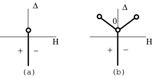
Figure 2: Possible phase diagrams for the zero temperature phase transition: (a) continuous transition, (b) first-order transition. $+$ and $-$ are the coexisting ordered phases and $0$ is the coexisting disordered phase in (b).

where $\psi=m(H\rightarrow 0^{+})$ and $\beta$ is the magnetization exponent. Figure 2a illustrates the continuous transition scenario in the zero temperature $H$-$\Delta$ plane with a critical point at the end of a line of first-order transitions. Another possibility is that the zero temperature transition is first-order. A possible scenario is illustrated with Fig. 2b. Here $(H=0,\Delta=\Delta_{c})$ is a point of coexistence of two ordered phases and one disordered phase. The magnetization of the coexisting ordered phases is nonzero while the disordered phase has zero magnetization. There will also be a nonzero “latent heat” at the transition. Although entropy is ill-defined at zero temperature, it is reasonable to define latent heat in terms of a discontinuity in the bond energy, $e$, between the ordered and disordered phases.

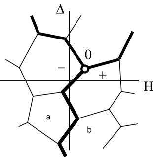
Figure 3: Ground states for a given realization of normalized random fields, $\{h_{i}\}$. Coexistence lines between ground states with very different magnetizations are shown as thick lines on the plot, the finite-size critical point is shown as an open circle and the three coexisting states at the finite-size critical point are labeled $+$, $-$ and $0$ as described in the text.

The foregoing applies to infinite systems. The ground states of a typical finite system for a given realization of the random field are shown in Fig. 3. Each point in the $H$-$\Delta$ plane corresponds to a single ground state of the system. The set of points corresponding to a single ground state form a polygon since, for a given spin configuration, the energy is linear in both $H$ and $\Delta$. In principle, there might be several degenerate ground states in a nonzero area of the $H$-$\Delta$ plane but, for a continuous distribution of random fields, the probability of exact degeneracy vanishes except along lines and at points. Along the edges between polygons the two ground states corresponding to each polygon are degenerate. Three ground states are degenerate at “triple points” where three edges meet. In principle, more than three ground states can be degenerate at a point but, for a continuous distribution of random fields, the probability of more than three degenerate ground states vanishes.

Degenerate ground states typically differ on a small fraction of spins but, corresponding to the first-order line of the infinite system, some degenerate ground states differ by a large fraction of the total number of spins. The bold lines in Fig. 3 correspond to large jumps in the magnetization. For $\Delta<\Delta_{c}$, there is a single jump between ground states with large positive and negative magnetization and the separation between these “phases” is the piecewise linear curve $H_{\rm coex}(\Delta)$. This coexistence line is close to but not coincident with the $\Delta$ axis. The spontaneous magnetization, $\psi$ is the magnetization of the positively magnetized ground states along $H_{\rm coex}$. As $\Delta_{c}$ is approached from below, $\psi$ decreases in steps at triple points. Since the net change in magnetization around a triple point is zero, the decrease in magnetization along $H_{\rm coex}$ is exactly the jump across the third edge or “lateral line” that defines the triple point. As the critical point is approached, the magnetization drops more precipitously so that the magnetization jump across the lateral line increases. We identify the finite-size “critical point” as the triple point with the largest jump across the lateral line. In Fig. 3 the finite-size critical point is shown as an open circle and the corresponding lateral line is also shown as thick line. The three states that are degenerate at the critical point are called the $+$, $-$ and $0$ states according to their relative magnetizations. If the transition were first-order these states would be the zero temperature analog of $+$ and $-$ ordered phases and the disordered phase that coexist at a thermal first-order transition.

One way to measure the discontinuity in the magnetization at the critical point is via the quantity, $m^{\ast}$,

$$m^{\ast}=\frac{1}{2}(m_{+}-m_{0})(m_{-}-m_{0})(m_{+}-m_{-})$$ (6)

where $m_{+}$, $m_{0}$ and $m_{-}$ are the magnetizations of the three coexisting critical ground states. Note that the same combination of three magnetizations is small at triple points away from the critical point, even along the first-order line.

Although the energy, ${\cal H}$, is a continuous function of $H$ and $\Delta$, the bond energy, $e$, has discontinuities across edges separating coexisting ground states. The bond energy along the coexistence line, $H_{\rm coex}(\Delta)$, is expected to increase monotonically as $\Delta$ increases with jumps across each lateral line. The largest discontinuity in the bond energy is expected at the finite-size critical point and the quantity $e^{\ast}$, is a measure of that discontinuity,

$$e^{\ast}=\frac{1}{2}(e_{+}+e_{-})(e_{0}-e_{+})(e_{0}-e_{-})$$ (7)

where $e_{+}$, $e_{-}$ and $e_{0}$ are the bond energies of the $+$, $-$ and $0$ states, respectively.

If the phase transition is continuous, both $m^{\ast}$ and $e^{\ast}$ must approach zero as the system size goes to infinity while if the transition is first-order, these quantities will saturate at nonzero values. Furthermore, if the transition is continuous, we propose the following finite-size scaling behavior for the disorder averages of these quantities,

$$\overline{m^{\ast}}\sim L^{-3\beta/\nu}$$ (8)

and

$$\overline{e^{\ast}}\sim L^{-2(1-\alpha)/\nu}$$ (9)

where $L$ is the linear size of the system, $\alpha$ is the specific heat exponent, $\beta$ is the magnetization exponent and $\nu$ is the correlation length critical exponent. The finite-size scaling hypothesis for the magnetization is essentially identical to the standard finite-size scaling hypothesis except that the measurement is made at a point that is fine-tuned for the given realization of disorder rather than at the infinite system size critical point. The finite-size scaling for the bond energy energy is more difficult to motivate. First, at zero temperature free energy and energy are identical and entropy and specific heat are not well-defined. It is reasonable to suppose that the derivatives of energy with respect to $J$ at zero temperature have the same singularities as the derivatives of the free energy with respect to temperature at nonzero temperature. Thus, from Eq. (1), bond energy plays the role of entropy and its derivative with respect to $J$ plays the role of specific heat. The conventional finite-size scaling hypothesis for the specific heat is

$$C(T)\sim L^{\alpha/\nu}\tilde{C}((T-T_{c})L^{1/\nu})$$ (10)

If the specific heat is integrated across the finite-size rounding region defined by $|T-T_{c}|<L^{-1/\nu}$ we obtain the finite-size “latent heat”, $l$ of the transition,

$$l\sim L^{-(1-\alpha/)\nu}$$ (11)

At zero temperature, this latent heat is replaced by the discontinuity in the the bond energy. Furthermore, since the bond energy changes at a discrete set of discontinuities, we propose that a finite fraction of the latent heat is concentrated at the triple point with the largest discontinuity, i.e. the point we have identified as the finite-size critical point. Since $e^{\ast}$ measures the square of the latent heat at the finite-size critical point, we obtain Eq. (9).

III Simulation method

The main goal of our simulations is to find and measure the properties of the zero temperature, finite-size critical point. The finite-size critical point is defined as the triple point with the largest jump in the magnetization between all three coexisting states. To find it we carry out an iterative search using a method similar to the one described in Ref.  Frontera et al. (2000). First, a point in the ordered phase on the first-order line is located. For example, in Fig.  3 we locate ground states “a” and “b” and a point on the coexistence line between them. Next, the first-order line is followed in the direction of increasing $\Delta$ from one triple point to the next. In the example of Fig.  3 the triple point where “a”, “b ”and “+” are degenerate is located first. At each triple point, the continuation of the first-order line (in this example, between “a” and “+”) and the lateral line (between “b” and “+” ) are identified according to the relative sizes of the discontinuities in the magnetization across the lines. The sequence of triple points is recorded and the triple point with the largest discontinuity in the magnetization across the lateral line is identified as the finite-size critical point.

The most difficult computational problem in carrying out this program is to find the ground state for given values of $\Delta$, $H$ and $\{h_{i}\}$. Finding ground states can be reduced to the problem of finding the maximum flow on a graph Ogielski (1986); Angles d’Auriac et al. (1985) for which there exists polynomial time algorithms. We use the push-relabel network flow algorithm Goldberg and Tarjan (1988); Cherkassky and Goldberg (1997), implemented in Goldberg as version hi_pr, to find ground states.

Let’s now describe in detail the two subroutines of the search algorithm. Subroutine 1 finds a point on the first-order line separating the positively and negatively ordered phases. Two ground states are found deep in the ordered phases at values $\Delta_{0}=2.2$ and $H=\pm 0.1$. Once these ground states are found, the algorithm calculates the value of $H$ where these two states are degenerate along the $\Delta=\Delta_{0}$ line. This point of degeneracy is easily found by the solution of two simultaneous linear equations since once ${\cal H}$, $e$ and $m$ are known for a given spin configuration at some point in the $H-\Delta$ plane, the value of ${\cal H}$ for that spin configuration at any other point is linearly related. At this point of degeneracy the ground state is calculated. If the result is either of the two original ground states then we have found a point on the first-order line. If the ground state at the point of degeneracy is not one of the original states then a new point of degeneracy is found between this new state and one of the original two states. The choice of which original state to pick is made by the criterion that the jump in the magnetization between it and the new state is biggest. This process is repeated until the first-order line is found.

Subroutine 2 follows the first-order line found in subroutine 1 until the first triple point is found in the direction of increasing $\Delta$. From the point found by subroutine 1 on the first-order line a new point is picked by moving in the direction of the first-order line and increasing $\Delta$ by $0.1$. On Fig. 3 this new point is on an imagined continuation of the thick line between “a” and “b” in the direction of $+$. An increase of $0.1$ in $\Delta$ has proved to be sufficiently large to extend to a new ground state for all system sizes studied. Subroutine 2 is similar to subroutine 1 except that original ground states are always retained in the iteration and a sequence of new ground states with decreasing values of $\Delta$ are generated. At each step in the iteration, the point of degeneracy is found between the new and the old states and the ground state is computed at that point. If the ground state is one of already identified states then the triple point has been found otherwise the iteration is repeat. Call this first triple point $(H_{1},\Delta_{1})$.

The triple point $(H_{1},\Delta_{1})$ defines three lines of coexistence, one of these lines is the previously identified first-order line. The jumps in magnetization across the other two lines are measured. The line with the smaller jump in magnetization is called the “lateral line” and the remaining line with the large jump in magnetization is continuation of the first-order line. The jump across the lateral line is recorded and subroutine 2 is invoked again to find the next triple point along the first-order line. By repeating this set of steps many times, a sequence of triple points $(H_{i},\Delta_{i})$ are identified. The triple point with the largest jump across the lateral line is identified as the finite-size critical point, $(H^{\ast},\Delta^{\ast})$.

We note that while the critical point is identified by the size of the jumps in the magnetization, in every case that we examined it also has the largest discontinuity in the bond energy. In principle, a definition of the finite-size critical point based on the bond energy discontinuity might sometimes yield a different triple point.

A typical running time for finding the ground state for a system of $L=10$ is $6\times 10^{-5}$ sec/spin on a Pentium III 750MHz machine. The total running time of the entire algorithm for the same system size is approximately one minute. We simulated systems of size up to $L=60$. The number of realizations of disorder range from 23 to 126 for different system sizes. The small number of realizations are a consequence of the fact that many ground states must be explored for each realization of disorder to find the finite-size critical point.

IV Results

Figure 4 shows the critical magnetization discontinuity $m^{\ast}$ as a function of system size $L$. Clearly this plot, together with Eq. (8) suggests that the magnetization discontinuity at the critical point does not decrease with $L$ which can be interpreted either as a first-order transition or a value of $\beta$ very near zero. The quality of the data is not sufficient to make a useful measurement of $\beta$. Figure 5 shows the finite-size scaling of the critical bond energy discontinuity $e^{\ast}$. A fit of the form:

$$e^{\ast}=a+bL^{-c}$$ (12)

yields $a=0.007\pm 0.005$, $b=21\pm 5$ and $c=1.7\pm 0.1$. It is clear that $e^{\ast}$ vanishes as power of $L$. This result is a clear indication of a continuous transition. Assuming a=0, we obtain a fit, shown in Fig. 5, of the form:

$$e^{\ast}=bL^{-c}$$ (13)

with $b=16.0\pm 2.6$ and $c=1.59\pm 0.05$. From the latter result and Eq. (9) we obtain $(1-\alpha)/\nu=0.80\pm 0.03$ (with $\chi^{2}=2.84$, $\chi^{2}/d.o.f.=0.57$ and $Q=0.73$). This result is in agreement with Middleton and Fisher’s valueMiddleton and Fisher (2002), $0.82\pm 0.02$.

The correlation length exponent $\nu$ and the infinite size critical disorder strength, $\Delta_{c}$ can be obtained from the finite size scaling of $\Delta^{\ast}$. The fit in Fig. 6 is:

$$\Delta^{\ast}=\Delta_{c}+bL^{-1/\nu}$$ (14)

with $\Delta_{c}=2.29\pm 0.02$, $b=4.1\pm 0.6$ and $\nu=1.1\pm 0.1$ (with $\chi^{2}=2.79$, $\chi^{2}/d.o.f.=0.69$ and $Q=0.59$). This result is in relatively good agreement with recent results in the literature as shown on Table 1. The value of $\nu$ is somewhat smaller than the recent values in Refs. Hartmann and Young (2001); Middleton and Fisher (2002) which may result from the use of a smaller maximum system size in our study. Combining our results for $\nu$ and for $(1-\alpha)/\nu$ yields $\alpha=0.1\pm 0.1$. Using the larger values of $\nu$ from Refs. Hartmann and Young (2001); Middleton and Fisher (2002) gives slightly negative values of $\alpha$. In any case, within the uncertainties, our results are consistent with modified hyperscaling.

V Discussion

The main result of this study is a new measurement of the specific heat exponent of the RFIM. Our result is a value of $\alpha$ near zero that is consistent with the modified hyperscaling relation and the recent simulation results by Middleton and Fisher Middleton and Fisher (2002). It is not clear why a very similar measurement by Hartmann and Young Hartmann and Young (2001) give $\alpha$ quite negative. Our value of $\alpha$ and that of Ref. Middleton and Fisher (2002) are based directly on the finite-size scaling of the bond energy at the critical point whereas in Ref.  Hartmann and Young (2001) the average bond energy is numerically differentiated to obtain the specific heat and the finite-size scaling of the peak is used to obtain $\alpha$.

Ref.		$\Delta$		$\nu$		$(1-\alpha)/\nu$		$\alpha$
This work		2.29(2)		1.1(1)		0.80(3)		0.12
Hartmann and Young (2001)		2.28(1)		1.36(1)		1.20		$-0.63(7)$
Middleton and Fisher (2002)		2.270(4)		1.37(9)		0.82(2)		$-0.12$
Angles d’Auriac and Sourlas (1997)		2.26(1)		1.22(6)
Hartmann and Nowak (1999)		2.29(4)		1.19(8)
Nowak et al. (1998)		2.37(5)		1.0(1)		1.55		$-0.55(20)$

Table 1: A summary of recent zero temperature estimates of $\Delta_{c}$, $\nu$, $(1-\alpha)/\nu$, and $\alpha$. For $\alpha$ and $(1-\alpha)/\nu$ the value without error estimated is derived from the other, directly measured, value and the same authors’ value of $\nu$.

Figure 1: Phase diagram of the random field Ising model. The ordered ferromagnetic phase is labeled $F$ and the disordered paramagnetic phase is labeled $P$. The curve is a line of phase transitions.

Figure 4: The magnetization discontinuity at the critical point, $m^{\ast}$ vs. system size, $L$.

Figure 5: Log-log plot of bond energy discontinuity at the critical point, $e^{\ast}$ vs. the system size, $L$. The solid line is a fit as described in the text.

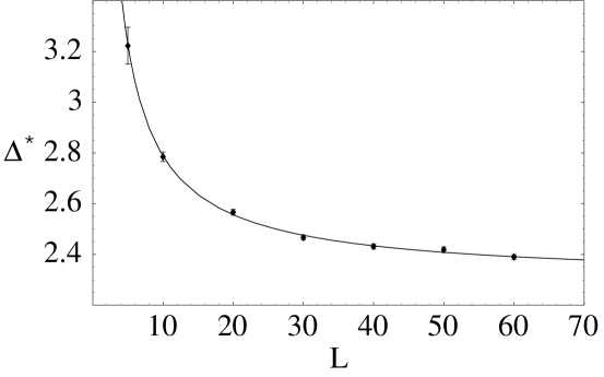
Figure 6: The critical strength of randomness, $\Delta^{\ast}$ vs. system size, $L$. The solid line is a fit as described in the text.