Statistical Error in Particle Simulations
of Hydrodynamic Phenomena

Abstract

We present predictions for the statistical error due to finite sampling in the presence of thermal fluctuations in molecular simulation algorithms. Specifically, we establish how these errors depend on Mach number, Knudsen number, number of particles, etc. Expressions for the common hydrodynamic variables of interest such as flow velocity, temperature, density, pressure, shear stress and heat flux are derived using equilibrium statistical mechanics. Both volume-averaged and surface-averaged quantities are considered. Comparisons between theory and computations using direct simulation Monte Carlo for dilute gases, and molecular dynamics for dense fluids, show that the use of equilibrium theory provides accurate results.

Keywords: Statistical error, sampling, fluctuations, Monte Carlo, hydrodynamics

1 Introduction

Recently much attention has been focused on the simulation of hydrodynamic problems at small scales using molecular simulation methods such as Molecular Dynamics (MD) [1, 2] or the direct simulation Monte Carlo (DSMC) [3, 4]. Molecular Dynamics is generally used to simulate liquids while DSMC is a very efficient algorithm for simulating dilute gases. In molecular simulation methods the connection to macroscopic observable fields, such as velocity and temperature, is achieved through averaging appropriate microscopic properties. The simulation results are therefore inherently statistical and statistical errors due to finite sampling need to be fully quantified.

Though confidence intervals may be estimated by measuring the variance of these sampled quantities, this additional computation can be burdensome and thus is often omitted. Furthermore, it would be useful to estimate confidence intervals a priori so that one could predict the computational effort required to achieve a desired level of accuracy. For example, it is well known that obtaining accurate hydrodynamic fields (e.g., velocity profiles) is computationally expensive in low Mach number flows so it is useful to have an estimate of the computational effort required to reach the desired level of accuracy.

In this paper we present expressions for the magnitude of statistical errors due to thermal fluctuations in molecular simulations for the typical observables of interest, such as velocity, density, temperature, and pressure. We also derive expressions for the shear stress and heat flux in the dilute gas limit. Both volume averaging and flux averaging is considered, even though the measurement of the shear stress and heat flux through volume averaging is not exact unless the contribution of the impulsive collisions is accounted for. Although we make use of expressions from equilibrium statistical mechanics, the non-equilibrium modifications to these results are very small, even under extreme conditions [5]. This is verified by the good agreement between our theoretical expressions and the corresponding measurements in our simulations.

In addition to direct measurements of hydrodynamic fields, this analysis will benefit algorithmic applications by providing a framework were statistical fluctuations can be correctly accounted for. One example of such application is the measurement of temperature for temperature-dependent collision rates [16]; another example is the measurement of velocity and temperature for the purpose of imposing boundary conditions [20]. Additional examples include hybrid methods [11, 14] where the coupling between continuum and molecular fields requires both averaging of finite numbers of particles in a sequence of molecular realizations as well as the generation of molecular realizations, based on continuum fields, with relatively small numbers of particles (e.g., buffer cells).

In section 2 the theoretical expressions for the statistical error due to thermodynamic fluctuations are derived. These expressions are verified by molecular simulations, as described in section 3. The effect of correlations between samples in dilute gases is briefly discussed in section 4 and concluding remarks appear in section 5.

2 Statistical error due to thermal fluctuations

2.1 Volume-averaged quantities

We first consider the fluid velocity. In a particle simulation, the flow field is obtained by measuring the instantaneous center of mass velocity, $\mathbf{u}$, for particles in a statistical cell volume. The statistical mean value of the local fluid velocity, $\langle\mathbf{u}\rangle_{s}$, is estimated over $M$ independent samples. For steady flows, these may be sequential samples taken in time; for transient flows these may be samples from an ensemble of realizations. The average fluid velocity, $\langle\mathbf{u}\rangle$, is defined such that $\langle\mathbf{u}\rangle_{s}\rightarrow\langle\mathbf{u}\rangle$ as $M\rightarrow\infty$; for notational convenience we also write $\langle\mathbf{u}\rangle=\mathbf{u}_{0}$. Define $\delta u_{x}\equiv u_{x}-u_{x0}$ to be the instantaneous fluctuation in the $x$-component of the fluid velocity; note that all three components are equivalent. From equilibrium statistical mechanics [6],

$$\langle\delta u_{x}^{2}\rangle=\frac{kT_{0}}{mN_{0}}=\frac{a^{2}}{\gamma\mathrm{Ac}^{2}N_{0}}$$ (1)

where $N_{0}$ is the average number of particles in the statistical cell, $T_{0}$ is the average temperature, $m$ is the particle mass, $k$ is Boltzmann’s constant, $a$ is the sound speed, and $\gamma=c_{P}/c_{V}$ is the ratio of the specific heats. The acoustic number $\mathrm{Ac}=a/a^{i}$ is the ratio of the fluid’s sound speed to the sound speed of a “reference” ideal gas at the same temperature

$$a^{i}=\sqrt{\gamma kT/m}$$ (2)

Note that this reference ideal gas has a ratio of specific heats ($\gamma^{i}$) equal to the original fluid specific heat ratio, that is $\gamma^{i}=\gamma$ as shown in equation (2).

An alternative construction of (1) is obtained from the equipartition theorem [6]

$${\textstyle\frac{3}{2}}kT_{0}={\textstyle\frac{1}{2}}m\langle|\mathbf{c}-\mathbf{c}_{0}|^{2}\rangle={\textstyle\frac{1}{2}}m\langle((c_{x}-c_{x0})^{2}+(c_{y}-c_{y0})^{2}+(c_{z}-c_{z0})^{2})\rangle={\textstyle\frac{3}{2}}m\langle(c_{x}-c_{x0})^{2}\rangle$$ (3)

where $\mathbf{c}$ is the translational molecular velocity. For a non-equilibrium system, this expression defines $T_{0}$ as the average translational temperature. Note that $\mathbf{u}_{0}=\mathbf{c}_{0}$ and

$$\langle|\delta\mathbf{u}|^{2}\rangle=\frac{\langle|\mathbf{c}-\mathbf{c}_{0}|^{2}\rangle}{N_{0}}=\frac{3kT_{0}}{mN_{0}}.$$ (4)

The above expression also reminds us that the expected error in estimating the magnitude of the fluid velocity is $\sqrt{3}$ larger than in estimating a velocity component.

We may define a “signal-to-noise” ratio as the average fluid velocity over its standard deviation; from the above,

$$\frac{|u_{x0}|}{\sqrt{\langle\delta u_{x}^{2}\rangle}}=\mathrm{Ac}\,\mathrm{Ma}\sqrt{\gamma N_{0}}$$ (5)

where $\mathrm{Ma}=|u_{x0}|/a$ is the local Mach number based on the velocity component of interest. This result shows that for fixed Mach number, in a dilute gas simulation ($\mathrm{Ac}=1$), the statistical error due to thermal fluctuations cannot be ameliorated by reducing the temperature. However, when the Mach number is small enough for compressibility effects to be negligible, favorable relative statistical errors may be obtained by performing simulations at an increased Mach number (to a level where compressibility effects are still negligible).

The one-standard-deviation error bar for the sample estimate $\langle u_{x}\rangle_{s}$ is $\sigma_{u}=\sqrt{\langle\delta u_{x}^{2}\rangle}/\sqrt{M}$ and the fractional error in the estimate of the fluid velocity is

$$E_{u}=\frac{\sigma_{u}}{|u_{x0}|}=\frac{1}{\sqrt{MN_{0}}}\,\frac{1}{\mathrm{Ac}\,\mathrm{Ma}\sqrt{\gamma}},$$ (6)

yielding

$$M=\frac{1}{\gamma\mathrm{Ac}^{2}N_{0}\mathrm{Ma}^{2}E_{u}^{2}}.$$ (7)

For example, with $N_{0}=100$ particles in a statistical cell, if a one percent fractional error is desired in a $\mathrm{Ma}=1$ flow, about $M=100$ independent statistical samples are required (assuming $\mathrm{Ac}\approx 1$). However, for a $\mathrm{Ma}=10^{-2}$ flow, about $10^{6}$ independent samples are needed, which quantifies the empirical observation that the resolution of the flow velocity is computationally expensive for low Mach number flows.

Next we turn our attention to the density. From equilibrium statistical mechanics, the fluctuation in the number of particles in a cell is

$$\langle\delta N^{2}\rangle=-N^{2}\frac{kT_{0}}{V^{2}}\left(\frac{\partial V}{\partial P}\right)_{T}=\kappa_{T}N_{0}^{2}\frac{kT_{0}}{V}$$ (8)

where $V$ is the volume of the statistics cell and $\kappa_{T}\equiv-V^{-1}(\partial V/\partial P)_{T}$ is the isothermal compressibility. Note that for a dilute gas $\kappa_{T}=1/P$ so $\langle\delta N^{2}\rangle=N$ and, in fact, $N$ is Poisson random variable. The fractional error in the estimate of the density is

$$E_{\rho}=\frac{\sigma_{\rho}}{\rho_{0}}=\frac{\sigma_{N}}{N_{0}}=\frac{\sqrt{\langle\delta N^{2}\rangle}}{N_{0}\sqrt{M}}=\frac{\sqrt{\kappa_{T}kT_{0}}}{\sqrt{MV}}=\frac{\sqrt{\kappa_{T}/\kappa_{T}^{i}}}{\sqrt{MN_{0}}}$$ (9)

where $\kappa_{T}^{i}=V/N_{0}kT_{0}$ is the isothermal compressibility of the reference dilute gas ($\gamma^{i}=\gamma$) at the same density and temperature. Since $a\propto 1/\sqrt{\kappa_{T}}$,

$$E_{\rho}=\frac{1}{\sqrt{MN_{0}}}\,\frac{1}{\mathrm{Ac}}$$ (10)

Note that for fixed $M$ and $N_{0}$, the error decreases as the compressibility decreases (i.e., as the sound speed increases) since the density fluctuations are smaller.

Let us now consider the measurement of temperature. First we should remark that the measurement of instantaneous temperature is subtle, even in a dilute gas. But given that temperature is measured correctly, equilibrium statistical mechanics gives the variance in the temperature fluctuations to be

$$\langle\delta T^{2}\rangle=\frac{kT_{0}^{2}}{c_{V}N_{0}}$$ (11)

where $c_{V}$ is the heat capacity per particle at constant volume. The fractional error in the estimate of the temperature is

$$E_{T}=\frac{\sigma_{T}}{T_{0}}=\frac{\sqrt{\langle\delta T^{2}\rangle}}{T_{0}\sqrt{M}}=\frac{1}{\sqrt{MN_{0}}}\,\sqrt{\frac{k}{c_{V}}}$$ (12)

Because the fluctuations are smaller, the error in the temperature is smaller when the heat capacity is large. Note that the temperature associated with various degrees of freedom (translational, vibrational, rotational) may be separately defined and measured. For example, if we consider only the measurement of the translational temperature, then the appropriate heat capacity is that of an ideal gas with three degrees of freedom, i.e. $c_{V}=\frac{3}{2}k$, corresponding to the three translational components.

Finally, the variance in the pressure fluctuations is

$$\langle\delta P^{2}\rangle=-kT_{0}\left(\frac{\partial P}{\partial V}\right)_{S}=\frac{\gamma kT_{0}}{V\kappa_{T}}$$ (13)

so the fractional error in the estimate of the pressure is

$$E_{P}=\frac{\sigma_{P}}{P_{0}}=\frac{\sqrt{\langle\delta P^{2}\rangle}}{P_{0}\sqrt{M}}=\frac{P_{0}^{i}}{P_{0}}\,\frac{\mathrm{Ac}\sqrt{\gamma}}{\sqrt{MN_{0}}}$$ (14)

where $P_{0}^{i}=N_{0}kT_{0}/V$ is the pressure of an ideal gas under the same conditions. Note that the error in the pressure is proportional to the acoustic number while the error in the density, eqn. (10), goes as $\mathrm{Ac}^{-1}$.

2.2 Shear stress and heat flux for dilute gases

The thermodynamic results in the previous section are general; in this section we consider transport quantities and restrict our analysis to dilute gases. In a dilute gas, the shear stress and heat flux are defined as

$$\tau_{xy0}=\langle\tau_{xy}\rangle=\langle\rho c_{x}c_{y}\rangle$$ (15)

and

$$q_{x0}=\langle q_{x}\rangle=\langle\frac{1}{2}\rho c_{x}c^{2}\rangle$$ (16)

respectively. This definition neglects the contribution of impulsive collisions to the transport within a given volume due to the negligible size of particles in the dilute limit. When, however, simulation methods such as DSMC are used to simulate a dilute gas that use a finite molecular size, a small error arises when momentum and energy transport is calculated in a volume averaged manner. In fact, this inconsistency has been addressed at the equation of state level by Alexander et al. [15] who pointed out that DSMC reproduces an ideal gas equation of state while simulating transport of a hard-sphere gas with molecules of finite size. Thus, under the assumption of a very dilute gas, the fluctuation in the (equilibrium) shear stress and heat flux in a volume $V$ containing $N_{0}$ particles can be calculated using the Maxwell-Boltzmann distribution. In equilibrium, the expected values of the above quantities are zero.

Using the definitions of shear stress and heat flux in terms of moments of the velocity distribution, direct calculation of the variance of the $x$-$y$ component of the stress tensor based on a single-particle distribution function gives

$$\langle\tau_{xy}^{2}\rangle = \langle(\rho c_{x}c_{y})^{2}\rangle$$ (17)

$$= \rho_{0}^{2}\;\langle(c_{x}c_{y})^{2}\rangle$$ (18)

$$= \frac{1}{4}\rho_{0}^{2}\left(\frac{2kT_{0}}{m}\right)^{2}=P_{0}^{2}$$ (19)

In obtaining the second equation we assumed $\langle c_{x}\rangle=\langle c_{y}\rangle=\langle(\rho-\rho_{0})c_{x}c_{y}\rangle=0$. For the $x$ component of the heat flux vector, we find

$$\langle q_{x}^{2}\rangle = \langle(\frac{1}{2}\rho c_{x}c^{2})^{2}\rangle$$ (20)

$$= \rho_{0}^{2}\;\langle(\frac{1}{2}c_{x}c^{2})^{2}\rangle$$ (21)

$$= \frac{35}{32}\rho_{0}^{2}\left(\frac{2kT_{0}}{m}\right)^{3}=\frac{35}{8}c_{\mathrm{m}}^{2}P_{0}^{2}$$ (22)

where $c_{\mathrm{m}}=\sqrt{2kT_{0}/m}$ the most probable particle speed and we have assumed $\langle c_{x}\rangle=\langle c_{y}\rangle=\langle(\rho-\rho_{0})c^{2}\rangle=0$. Note that in equilibrium for a cell containing $N_{0}$ particles, the variance of the mean is given by $\langle\delta\tau_{xy}^{2}\rangle=\langle\tau_{xy}^{2}\rangle/N_{0}$ and $\langle\delta q_{x}^{2}\rangle=\langle q_{x}^{2}\rangle/N_{0}$ for the shear stress and heat flux respectively.

In order to derive expressions for the relative fluctuations we need expressions for the magnitude of the fluxes. We are only able to provide closed form expressions for the latter in the continuum regime where

$$\tau_{xy}=\mu\left(\frac{\partial u_{x}}{\partial y}+\frac{\partial u_{y}}{\partial x}\right)$$ (23)

and

$$q_{x}=-\kappa\frac{\partial T}{\partial x}$$ (24)

where $\mu$ is the coefficient of viscosity and $\kappa$ is the thermal conductivity. Above Knudsen numbers of $\mathrm{Kn}\approx 0.1$, it is known that these continuum expressions are only approximate and better results are obtained using more complicated formulations from kinetic theory (e.g., Burnett’s formulation). Here, the Knudsen number is defined as $\mathrm{Kn}=\lambda/\ell$ and the mean free path as

$$\lambda=\frac{8}{5\sqrt{\pi}}\frac{c_{\mathrm{m}}\mu}{P_{0}}$$ (25)

Note that this expression for the mean free path simplifies to the hard sphere result when the viscosity is taken to be that of hard spheres.

Using (23) and (24) we find that in continuum flows, the relative fluctuations in the shear stress and heat flux are given by

$$E_{\tau}=\frac{\sqrt{\langle\delta\tau_{xy}^{2}\rangle}}{|\tau_{xy0}|\sqrt{M}}=\frac{16}{5\sqrt{2\pi\gamma}}\frac{1}{\mathrm{Kn}\,\mathrm{Ma}_{*}}\frac{1}{\sqrt{N_{0}M}}\left|\frac{\partial u_{x}^{*}}{\partial y^{*}}+\frac{\partial u_{y}^{*}}{\partial x^{*}}\right|^{-1}$$ (26)

and

$$E_{q}=\frac{\sqrt{\langle\delta q_{x}^{2}\rangle}}{|q_{x0}|\sqrt{M}}=\frac{8\sqrt{35}}{5\sqrt{2\pi}}\frac{\mathrm{Pr}(\gamma-1)}{\gamma}\frac{T}{\Delta T}\frac{1}{\mathrm{Kn}}\frac{1}{\sqrt{N_{0}M}}\left|\frac{\partial T^{*}}{\partial x^{*}}\right|^{-1}$$ (27)

respectively. Here, stars denote non-dimensional quantities: $u^{*}=u_{0}/\tilde{u}$, $T^{*}=T/\Delta T$ and $x^{*}=x/\ell$, where $\tilde{u}$, $\Delta T$, and $\ell$ are characteristic velocity, temperature variation and length. The Mach number $\mathrm{Ma}_{*}$ is defined with respect to the characteristic velocity $\tilde{u}$ rather than the local velocity as in eq. (6).

If viscous heat generation is responsible for the temperature differences characterized by $\Delta T$, then it is possible to express equation (27) in the following form

$$E_{q}=\frac{\sqrt{\langle\delta q_{x}^{2}\rangle}}{|q_{x0}|\sqrt{M}}=\frac{8\sqrt{35}}{5\gamma\sqrt{2\pi}}\frac{\mathrm{Br}}{\mathrm{Kn}\mathrm{Ma}^{2}_{*}}\frac{1}{\sqrt{N_{0}M}}\left|\frac{\partial T^{*}}{\partial x^{*}}\right|^{-1}$$ (28)

The Brinkman number

$$\mathrm{Br}=\frac{\mu\tilde{u}^{2}}{\kappa\Delta T},$$ (29)

is the relevant non-dimensional group that compares temperature differences due to viscous heat generation to the characteristic temperature differences in the flow. (It follows that if viscous heat generation is responsible for the temperature changes, $\mathrm{Br}\approx 1$.)

It is very instructive to extend the above analysis to equation (12). If we define the relative error in temperature with respect to the temperature changes rather than the absolute temperature, we obtain

$$E_{\Delta T} = \frac{\sigma_{T}}{\Delta T}=\frac{\sqrt{\langle\delta T^{2}\rangle}}{\Delta T\sqrt{M}}=\frac{T_{0}}{\Delta T\sqrt{MN_{0}}}\,\sqrt{\frac{k}{c_{V}}}$$ (30)

$$= \frac{1}{\mathrm{Pr}(\gamma-1)}\frac{\mathrm{Br}}{\mathrm{Ma}_{*}^{2}}\frac{1}{\sqrt{MN_{0}}}\,\sqrt{\frac{k}{c_{V}}}$$ (31)

where again, if viscous heat generation is the only source of heat, $\mathrm{Br}\approx 1$. The above development shows that resolving the temperature differences or heat flux due to viscous heat generation is very computationally inefficient for low speed flow since for a given expected error $E_{\Delta T}$ we find that the number of samples $M\propto\mathrm{Ma}^{-4}_{*}$.

Comparison of equations (6) and (26) and equations (12) and (27) reveals that

$$E_{\tau}\sim\frac{E_{u}}{\mathrm{Kn}}$$ (32)

and

$$E_{q}\sim\frac{E_{\Delta T}}{\mathrm{Kn}}$$ (33)

since the non-dimensional gradients will be of order one. As the above equations were derived for the continuum regime ($\mathrm{Kn}<0.1$), it follows that the relative error in these moments is significantly higher. This will also be shown to be the case in the next section when the shear stress and heat flux are evaluated as fluxal (surface) quantities. This has important consequences in hybrid methods [14, 11], as coupling in terms of state (Dirichlet) conditions is subject to less variation than coupling in terms of flux conditions.

2.3 Fluxal quantities

In this section we predict the relative errors in the fluxes of mass and heat as well as the components of the stress tensor, when calculated as fluxes across a reference surface. Our analysis is based on the assumption of an infinite, ideal gas in equilibrium. In this case, it is well known that the number of particles, $N_{i}$, in each infinitessimal cell $i$ is an independent Poisson random variable with mean and variance,

$$\langle N_{i}\rangle=\langle\delta N_{i}^{2}\rangle=n\Delta x_{i}\Delta y_{i}\Delta z_{i},$$ (34)

where $n=\rho/m$ is the particle number density.

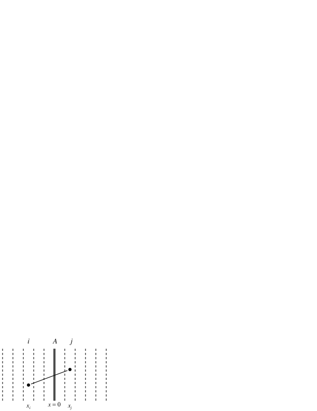
Figure 1: Schematic particle motion crossing surface $A$.

In the Appendix, it is shown that, more generally, all number fluctuations are independent and Poisson distributed. In particular, the number of particles, $N^{+}_{ij}$, leaving a cell $i$ at position $(x_{i},y_{i},z_{i})$, crossing a surface, and arriving in another cell $j$ at position $(x_{j},y_{j},z_{j})$ after a time $\Delta t$ (see Figure 1) is also an independent Poisson random variable. Its mean and variance are given by

$$\langle N_{ij}^{+}\rangle=\langle(\delta N_{ij}^{+})^{2}\rangle=P_{ij}\langle N_{i}\rangle$$ (35)

where

$$P_{ij}=P(x_{ij},y_{ij},z_{ij})\Delta x_{j}\Delta y_{j}\Delta z_{j},$$ (36)

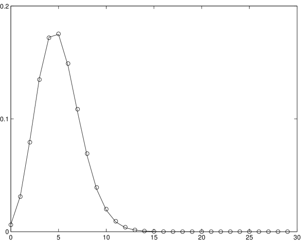
Figure 2: Probability disrtibution of number of particles crossing a surface in the gas. The circles denote equilibrium DSMC results and the solid line shows a Poisson distribution with mean $\langle N\rangle$ based on the equilibrium result $\langle J^{+}\rangle=nc_{\mathrm{m}}/2\sqrt{\pi}$.

is the probability that a particle makes the transition, which depends only upon the relative displacements, $x_{ij}=x_{j}-x_{i}$, $y_{ij}=y_{j}-y_{i}$, and $z_{ij}=z_{j}-z_{i}$. These properties hold exactly for an infinite ideal gas in equilibrium, but they are also excellent approximations for most finite, dilute gases, even far from equilibrium, e.g. as shown by the DSMC result in Figure 2.

Without loss of generality we place a large planar surface of area $A$ at $x=0$. The flux in the positive direction, $J_{h}^{+}$, of any velocity-dependent quantity, $h(c_{x},c_{y},c_{z})$, can be expressed as a sum of independent, random contributions from different cells $i$ and $j$ on opposite sides of the surface,

$$J_{h}^{+}=\frac{1}{A\Delta t}\sum_{x_{i}<0}\sum_{x_{j}>0}\sum_{y_{i}}\sum_{y_{j}}\sum_{z_{i}}\sum_{z_{j}}\bar{h}(x_{ij},y_{ij},z_{ij})N_{ij}^{+}$$ (37)

where $\bar{h}(x_{ij},y_{ij},z_{ij})=h(c_{x},c_{y},c_{z})$ is the same quantity expressed in terms of relative displacements during the time interval, $\Delta t$. We begin by calculating the mean flux. Taking expectations in Eq. (37), we obtain

$$\langle J^{+}_{h}\rangle = \frac{1}{A\Delta t}\sum_{x_{i}<0}\sum_{x_{j}>0}\sum_{y_{i}}\sum_{y_{j}}\sum_{z_{i}}\sum_{z_{j}}\bar{h}(x_{ij},y_{ij},z_{ij})\langle N_{i}\rangle P_{ij}$$ (38)

$$\sim \frac{1}{\Delta t}\sum_{x_{i}<0}\sum_{x_{j}>0}\sum_{y_{j}}\sum_{z_{j}}\bar{h}(x_{ij},y_{j},z_{j})n\Delta x_{i}P(x_{ij},y_{j},z_{j})\Delta x_{j}\Delta y_{j}\Delta z_{j},$$ (39)

where without loss of generality we have taken $y_{i}=z_{i}=0$ and also separately performed the sums parallel to the surface,

$$\sum_{y_{i}}\sum_{z_{i}}\Delta y_{i}\Delta z_{i}=A,$$

by invoking translational invariance and neglecting any edge effects, since $\langle c_{y}\rangle\Delta t,\langle c_{z}\rangle\Delta t=o(\sqrt{A})$ in the limit $\Delta t\rightarrow 0$ (taken below).

Passing to the continuum limit in Eq. (39) and letting $A\rightarrow\infty$, we arrive at an integral expression for the mean flux through an infinite flat surface,

$$\langle J^{+}_{h}\rangle = \frac{n}{\Delta t}\;\int^{0}_{-\infty}dx^{\prime}\;\int^{\infty}_{0}dx\;\int^{\infty}_{-\infty}dy\;\int^{\infty}_{-\infty}dz\;\bar{h}(x-x^{\prime},y,z)P(x-x^{\prime},y,z)$$ (40)

$$= \frac{n}{\Delta t}\;\int^{\infty}_{0}dx\;\int_{x}^{\infty}ds\;\int^{\infty}_{-\infty}dy\;\int^{\infty}_{-\infty}dz\;\bar{h}(s,y,z)P(s,y,z).$$

Since the integrand does not depend on $x$, switching the order of integration,

$$\langle J^{+}_{h}\rangle = \frac{n}{\Delta t}\;\int_{0}^{\infty}ds\;\int^{\infty}_{-\infty}dy\;\int^{\infty}_{-\infty}dz\;\bar{h}(s,y,z)P(s,y,z)\int_{0}^{s}dx$$ (41)

$$= n\;\int_{0}^{\infty}ds\;\int^{\infty}_{-\infty}dy\;\int^{\infty}_{-\infty}dz\;\bar{h}(s,y,z)P(s,y,z)\frac{s}{\Delta t}$$

produces a simple formula for the mean flux as a conditional average over the velocity distribution (with $c_{x}>0$),

$$\langle J^{+}_{h}\rangle=n\;\langle c_{x}\;h(c_{x},c_{y},c_{z})\rangle^{+}$$ (42)

in the limit $\Delta t\rightarrow 0$. For $h(c_{x},c_{y},c_{z})=m,mc_{x},mc_{y},mc_{z},\frac{1}{2}mc^{2}$ in the absence of a mean flow, we obtain,

$$\langle J_{m}^{+}\rangle = n\langle c_{x}\;m\rangle^{+}=\frac{\rho c_{\mathrm{m}}}{2\sqrt{\pi}}$$ (43)

$$\langle J_{xx}^{+}\rangle = n\langle c_{x}\;mc_{x}\rangle^{+}=\frac{\rho kT_{0}}{2m}=\frac{P_{0}}{2}$$ (44)

$$\langle J_{xy}^{+}\rangle = n\langle c_{x}\;mc_{y}\rangle^{+}=0\qquad\qquad\langle J_{xz}^{+}\rangle=n\langle c_{x}\;mc_{z}\rangle^{+}=0$$ (45)

$$\langle J_{e}^{+}\rangle = n\langle c_{x}\;{\textstyle\frac{1}{2}}mc^{2}\rangle^{+}=\frac{\rho c_{\mathrm{m}}^{3}}{2\sqrt{\pi}}$$ (46)

which are the well-known results for the expected one-sided fluxes of mass, momentum, and energy, respectively.

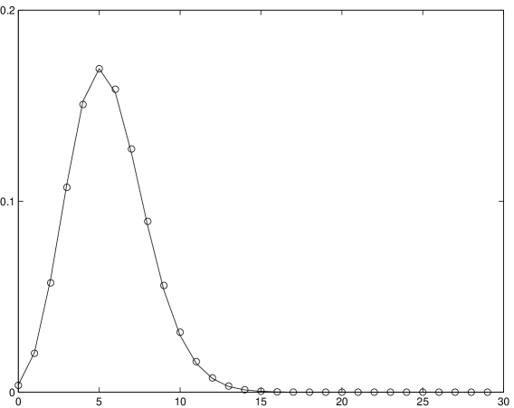
Figure 3: Probability disrtibution of number of particles crossing a surface in the gas in the presence of mean flow normal to the surface of interest. The circles denote equilibrium DSMC results and the solid line shows a Poisson distribution with mean $\langle N\rangle$ based on the particle flux in the presence of a mean flow.

Using the same formalism as above, we now derive a general formula for the variance of the flux, $\langle(\delta J^{+}_{h})^{2}\rangle$. For simplicity, we assume that the mean flow is zero normal to the reference surface, but our results below are easily extended to the case of a non-zero mean flow through the surface since Eq. (35) still holds in that case (see Figure 3). Taking the variance of Eq. (37) and using the independence of $\{N_{ij}^{+}\}$, we obtain

$$\langle(\delta J^{+}_{h})^{2}\rangle = \frac{1}{A^{2}\Delta t^{2}}\sum_{x_{i}<0}\sum_{x_{j}>0}\sum_{y_{i}}\sum_{y_{j}}\sum_{z_{i}}\sum_{z_{j}}\bar{h}(x_{ij},y_{ij},z_{ij})^{2}\langle(\delta N^{+}_{ij})^{2}\rangle$$ (47)

$$= \frac{1}{A^{2}\Delta t^{2}}\sum_{x_{i}<0}\sum_{x_{j}>0}\sum_{y_{i}}\sum_{y_{j}}\sum_{z_{i}}\sum_{z_{j}}\bar{h}(x_{ij},y_{ij},z_{ij})^{2}\langle N_{i}\rangle P_{ij}$$

Following the same steps above leading from Eq. (38) to Eq. (42) we arrive at the simple formula,

$$\langle(\delta J^{+}_{h})^{2}\rangle=\frac{n}{A\Delta t}\;\langle c_{x}\;h(c_{x},c_{y},c_{z})^{2}\rangle^{+}$$ (48)

in the continuum limit as $\Delta t\rightarrow 0$. The variance of the total flux is

$$\langle\delta J_{h}^{2}\rangle=\langle(\delta J_{h}^{+}+\delta J_{h}^{-})^{2}\rangle=\langle(\delta J_{h}^{+})^{2}\rangle+\langle(\delta J_{h}^{-})^{2}\rangle=2\langle(\delta J^{+}_{h})^{2}\rangle$$ (49)

since the one-sided fluxes through the surface, $J^{+}_{h}$ and $J^{-}_{h}$, are independent and identically distributed (with opposite sign).

Using this general result, we can evaluate the standard deviations of the fluxes above,

$$\sqrt{\langle\delta J_{m}^{2}\rangle} = \sqrt{\frac{\rho c_{\mathrm{m}}}{\sqrt{\pi}}}\sqrt{\frac{m}{A\Delta t}}$$ (50)

$$\sqrt{\langle\delta J_{xy}^{2}\rangle} = \sqrt{\frac{\rho c_{\mathrm{m}}^{3}}{2\sqrt{\pi}}}\sqrt{\frac{m}{A\Delta t}}$$ (51)

$$\sqrt{\langle\delta J_{e}^{2}\rangle} = \sqrt{\frac{3\rho c_{\mathrm{m}}^{5}}{2\sqrt{\pi}}}\sqrt{\frac{m}{A\Delta t}}$$ (52)

These formulae may be simplified by noting that

$$\langle J^{+}_{m}\rangle=\frac{mN^{+}}{A\Delta t}=\frac{\rho c_{\mathrm{m}}}{2\sqrt{\pi}}$$ (53)

where $N^{+}$ is the mean total number of particles crossing the reference surface in one direction in time $\Delta t,$, which yields

$$\sqrt{\langle\delta J_{m}^{2}\rangle} = \frac{\rho c_{\mathrm{m}}}{\sqrt{2\pi}}\frac{1}{\sqrt{N^{+}}}$$ (54)

$$\sqrt{\langle\delta J_{xy}^{2}\rangle} = \frac{\rho c^{2}_{\mathrm{m}}}{2\sqrt{\pi}}\frac{1}{\sqrt{N^{+}}}$$ (55)

$$\sqrt{\langle\delta J_{e}^{2}\rangle} = \sqrt{\frac{3}{\pi}}\frac{\rho c^{3}_{\mathrm{m}}}{2}\frac{1}{\sqrt{N^{+}}}$$ (56)

We may relate these to the results from the previous section by identifying $\langle\delta(\tau_{xy}^{f})^{2}\rangle=\langle\delta J_{xy}^{2}\rangle$ and $\langle\delta(q_{x}^{f})^{2}\rangle=\langle\delta J_{e}^{2}\rangle$, and additionally include the effect of $M$ (independent) samples in time. The superscript $f$ denotes fluxal measurement. By noting that transport fluxes are defined with respect to the rest frame of the fluid, it can be easily verified that the above relations hold in the case where a mean flow in directions parallel to the measuring surface exists, under the assumption of a local equilibrium distribution.

We can derive expressions for the relative expected error in the continuum regime in which models exist for the shear stress and heat flux. In this regime we find

$$E_{\tau}^{f}=\frac{\sqrt{\delta(\tau_{xy}^{f})^{2}}}{|\tau_{xy0}^{f}|\sqrt{M}} = \frac{16}{5\pi\sqrt{2\gamma}}\frac{1}{\mathrm{Kn}\;\mathrm{Ma}_{*}}\frac{1}{\sqrt{MN^{+}}}\left|{\frac{\partial u^{*}}{\partial y^{*}}}+{\frac{\partial v^{*}}{\partial x^{*}}}\right|^{-1}$$ (57)

and

$$E_{q}^{f}=\frac{\sqrt{\delta(q_{x}^{f})^{2}}}{|q_{x0}^{f}|\sqrt{M}} = \frac{16\sqrt{3}}{5\pi}\frac{\mathrm{Pr}(\gamma-1)}{\gamma}\frac{T}{\Delta T}\frac{1}{\mathrm{Kn}}\frac{1}{\sqrt{MN^{+}}}\left|\frac{\partial T}{\partial x^{*}}\right|^{-1}$$ (58)

$$= \frac{16\sqrt{3}}{5\gamma\pi}\frac{\mathrm{Br}}{\mathrm{Kn}\;\mathrm{Ma}^{2}_{*}}\frac{1}{\sqrt{MN^{+}}}\left|\frac{\partial T}{\partial x^{*}}\right|^{-1}$$ (59)

Comparing (57) with the corresponding expressions for volume-averaged stress tensor, (28), one finds that, aside from the numerical coefficients, the expressions differ only in the number of particles used, either $N^{+}$ or $N_{0}$; one finds a similar result for the heat flux.

2.4 Connection to Fluctuating Hydrodynamics

Fluctuating hydrodynamics, as developed by Landau, approximates the stress tensor and heat flux as white noises, with variances fixed by matching equilibrium fluctuations. In this section we identify the connection between Landau’s theory and the variances of fluxes obtained in section 2.2.

Landau introduced fluctuations into the hydrodynamic equations by adding white noise terms to the stress tensor and heat flux [17] (in the spirit of Langevin’s theory of Brownian motion [19]). The amplitudes of these noises are fixed by evaluating the resulting variances of velocity and temperature and matching with the results from equilibrium statistical mechanics [18]. For example, in Landau’s formulation the total heat flux in the $x$-direction is $q_{x}^{\mathrm{L}}=-\kappa\partial T/\partial x+g_{x}$ where the first term on the r.h.s. is the deterministic part of the flux and the second is the white noise term. The latter has mean zero and time correlation given by the following expression

$$\langle g_{x}(t)g_{x}(t^{\prime})\rangle=\frac{2k\kappa T^{2}}{V}\delta(t-t^{\prime})$$ (60)

Note that at a steady state the deterministic part is constant so $\langle\delta q_{x}^{\mathrm{L}}(t)\delta q_{x}^{\mathrm{L}}(t^{\prime})\rangle=\langle g_{x}(t)g_{x}(t^{\prime})\rangle$.

On the other hand, recall from eqn. (22),

$$\langle\delta q_{x}^{2}\rangle=\frac{35}{32}\frac{\rho^{2}c_{\mathrm{m}}^{6}}{N_{0}}$$ (61)

The question naturally arises: how does one reconcile (60) and (61)? Note that the fluctuating hydrodynamics expression contains the thermal conductivity, which depends on the particle interaction (e.g., for hard-spheres $\kappa$ depends on the particle diameter) while the kinetic theory expression is independent of this interaction.

The key lies in identifying the $\delta$-function with a decay time, $t_{d}$, that is vanishingly small at hydrodynamic scales. Specifically, we may write

$$\delta(t-t^{\prime})\rightarrow\left\{\begin{array}[]{cc}t_{d}^{-1}&|t-t^{\prime}|<t_{d}\\ 0&\mathrm{otherwise}\end{array}\right.$$ (62)

so

$$\langle g^{2}_{x}(t)\rangle=\frac{2k\kappa T^{2}}{t_{d}V}=\frac{\kappa V}{2kN_{0}c_{\mathrm{m}}^{2}t_{d}}\frac{\rho^{2}c_{\mathrm{m}}^{6}}{N_{0}}$$ (63)

Comparing with the above gives

$$t_{d}=\frac{16}{35}\frac{\kappa V}{kN_{0}c_{\mathrm{m}}^{2}}$$ (64)

For a hard sphere gas, $\kappa=\frac{5}{2}c_{V}\mu$ so using (25) we may write this as,

$$t_{d}=\frac{15\sqrt{\pi}}{28}\frac{\lambda}{c_{\mathrm{m}}}$$ (65)

For other particle interactions the coefficients will be slightly different but in general $t_{d}\approx\lambda/c_{\mathrm{m}}$, thus it is approximately equal to the molecular collision time. In conclusion, the two formulations are compatible once the white noise approximation in fluctuating hydrodynamics is justified by the fact that the hydrodynamic time scale is much longer than the kinetic (i.e., collisional) time scale. Landau’s construction provides a useful hydrodynamic approximation for $g_{x}$ but (61) is the actual variance of the heat flux.

3 Simulations

3.1 Dilute Gases

We performed DSMC simulations to verify the validity of the expressions derived above. Standard DSMC techniques [3, 4] were used to simulate flow of gaseous argon (molecular mass $m=6.63\times 10^{-26}$ kg, hard sphere diameter $\sigma=3.66\times 10^{-10}$ m) in a two-dimensional channel (length $L$ and height $H$). The simulation was periodic in the $x$ direction (along the channel axis). The two walls at $y=-H/2$ and $y=H/2$ were fully accommodating and flat. The simulation was also periodic in the third (homogeneous) direction.

The average gas density was $\rho_{0}=1.78\mathrm{kg}/\mathrm{m}^{3}$ and in all calculations over 40 particles per cell were used. The cell size was $\Delta x=\lambda_{0}/3$ where $\lambda_{0}$ is the reference mean free path. The time step was $\Delta t=\lambda_{0}/(7.5c_{\mathrm{m}})$. For a discussion of the errors resulting from finite cell sizes and time steps see [8, 9, 10]. The fractional error in the simulations is obtained from the standard deviation of cell values in the $x$ and $z$ directions. To ensure that the samples were independent, samples were taken only once every 250 time steps. To ensure that the system was in its steady state the simulation was run for $10^{6}$ time steps before sampling was started.

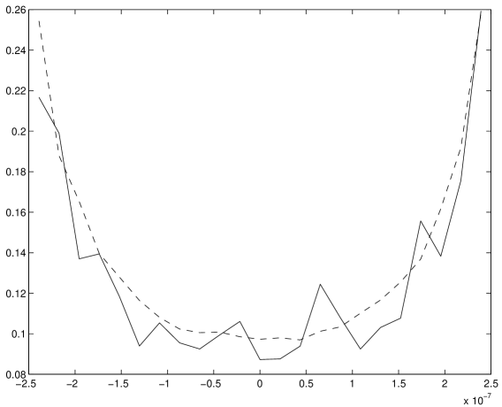
Figure 4: Fractional error in velocity for Poiseuille flow in a channel as a function of the transverse channel coordinate, $y$. The dashed line denotes equation (6) and the solid line denotes DSMC simulation results.

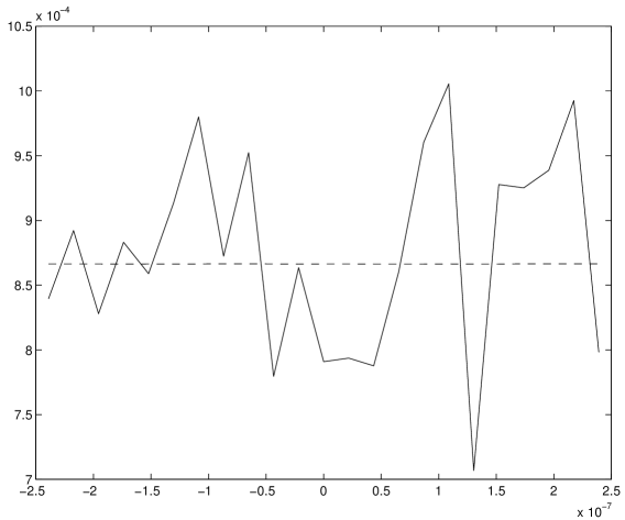
Figure 5: Fractional error in density for Poiseuille flow in a channel as a function of the transverse channel coordinate, $y$. The dashed line denotes equation (10) and the solid line indicates DSMC simulation results.

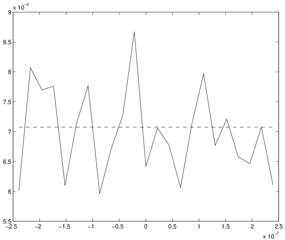
Figure 6: Fractional error in temperature for Poiseuille flow in a channel as a function of the transverse channel coordinate, $y$. The dashed line denotes equation (12) and the solid line indicates DSMC simulation results.

A constant acceleration was applied to the particles to produce Poiseuille flow in the $x$ direction with maximum velocity at the centerline $u_{0}^{\mathrm{max}}\approx 2$ m/s. Figures 4, 5, and 6 show good agreement between the theoretical expressions from section 2 and simulation measurements for the fractional error in velocity, density and temperature, respectively. The fractional error in the velocity measurement is minimum at the centerline since the Poiseuille velocity profile is parabolic and maximum at the centerline, (see Fig. 4). The density and temperature were nearly constant across the system so the fractional errors in these quantities are also nearly constant.

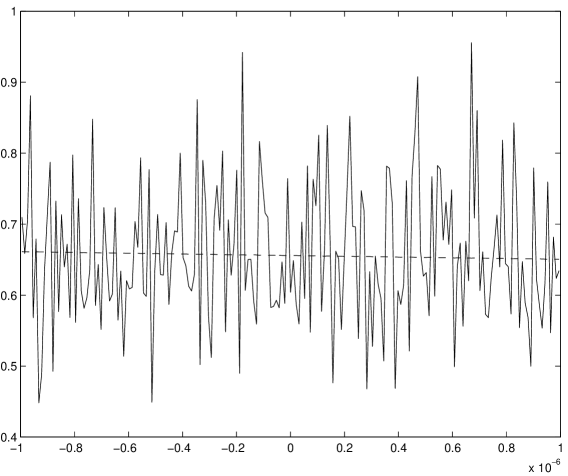
Figure 7: Fractional error in the shear stress $\tau_{xy}$ for Couette flow in a channel as a function of the transverse channel coordinate, $y$. The dashed line denotes equation (26) and the solid line indicates DSMC simulation results.

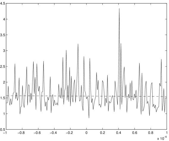
Figure 8: Fractional error in the shear stress for Couette flow in a channel as a function of the transverse channel coordinate, $y$. The dashed line denotes equation (57) and the solid line indicates DSMC simulation results.

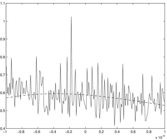
Figure 9: Fractional error in the heat flux for “Tempearture Couette” in a channel as a function of the transverse channel coordinate, $y$. The dashed line denotes equation (27) and the solid line indicates DSMC simulation results.

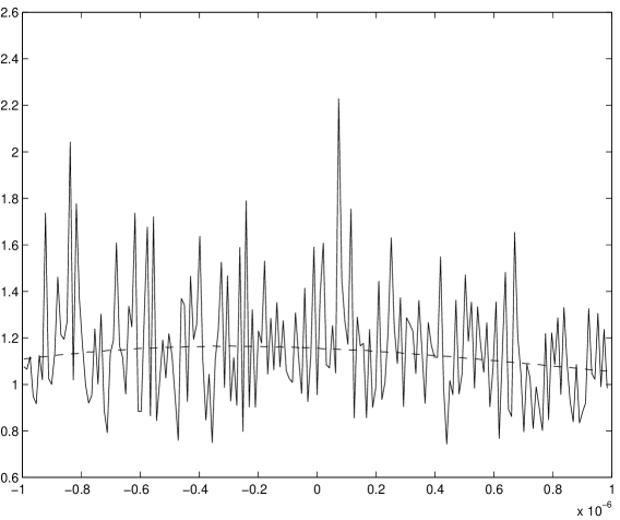
Figure 10: Fractional error in the heat flux for “Temperature Couette” in a channel as a function of the transverse channel coordinate, $y$. The dashed line denotes equation (59) and the solid line indicates DSMC simulation results.

The expressions for shear stress and heat flux were verified using Couette (walls at equal temperature with different velocities) and “temperature” Couette (walls at zero velocity with different temperatures) calculations respectively. In these calculations, very small cell sizes ($\Delta x=\lambda/6$) and time steps $(\Delta t=\lambda/(30c_{\mathrm{m}}))$ were used in order to minimize the discrepancy between the volume-averaged and surface-averaged shear stress and heat flux [8]. The system was equilibrated for $10^{6}$ time steps and samples were taken every 50 time steps. The momentum and energy fluxes de-correlate faster than the conserved hydrodynamic variables, such as density, so independent samples are obtained after fewer time steps (see section 4). Good agreement is found between the theoretical results and simulation measurements for volume averaged and fluxal quantities, as shown in figures 7, 8, 9, 10.

A final note: In DSMC simulations one considers each particle as “representing” a large number of molecules in the physical system. In all the expressions given above, $N_{0}$ and $N^{+}$ relates to the number of particles used by the simulation so the fluctuations can be reduced by using larger numbers of particles (i.e., using a lower molecule-to-particle ratio).

3.2 Dense fluids

We performed molecular dynamics simulations to test the validity of equations (6), (10), (12) for dense fluids. A similar geometry to the dilute gas simulations described above was used but at a significantly higher density. In particular, we simulated liquid argon ($\sigma_{LJ}=3.4\times 10^{-10}$m, $\varepsilon_{LJ}=119.8k_{b}$) at $T=240K$ and $\rho=860Kg/\mathrm{m}^{3}$ in a two-dimensional channel with the $x$ and $z$ directions periodic. The channel height was $H=69.7\sigma_{LJ}$. The wall molecules were connected to fcc lattice sites through springs and interacted with the fluid through a Lennard-Jones potential with the same parameters. The spring constant $k_{s}=460\varepsilon\sigma^{-2}$ was chosen in the way that root mean square displacement of wall atoms around their equilibrium position at the simulated temperature was well below the Lindermann criterion for the melting point of a solid. The length and depth of the system was $28\sigma_{LJ}$ and $29.1\sigma_{LJ}$ in the $x$ and $z$ directions respectively. A constant force $f=8\times 10^{-5}\varepsilon/\sigma_{LJ}$ per particle was used to generate a velocity field with a maximum velocity of approximately $13$ m/s.

In order to calculate the fluctuation of density, temperature and velocity, we divided the simulation cell into 13 layers in the $y-$direction with a height $\Delta y=4.6396\sigma$. We further divided each layer into $49$ cells, 7 in each of the $x$ and $z$ directions. The density, temperature and velocity in each cell were calculated in every $2000(0.005t_{LJ})$, where $t_{LJ}=\sqrt{m_{LJ}\sigma_{LJ}^{2}/\varepsilon_{LJ}}$. We have checked that this time interval is longer than the system’s correlation time such that samples taken between such intervals are independent. For each cell, $200$ samples are used to calculate the average density, temperature and velocity. The fluctuation was calculated for each layer using the 49 equivalent cells in the $x-z$ plane.

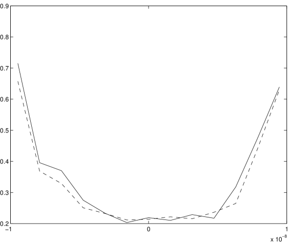
Figure 11: Fractional error in velocity for dense-fluid Poiseuille flow in a channel as a function of the transverse channel coordinate, $y$. The dashed line denotes equation (6) and the solid line denotes MD simulation results.

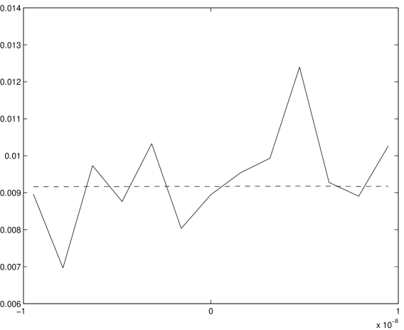
Figure 12: Fractional error in temperature for dense-fluid Poiseuille flow in a channel as a function of the transverse channel coordinate, $y$. The dashed line denotes equation (12) and the solid line indicates MD simulation results.

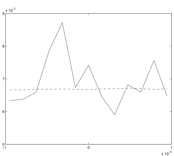
Figure 13: Fractional error in density for dense-fluid Poiseuille flow in a channel as a function of the transverse channel coordinate, $y$. The dashed line denotes equation (10) and the solid line indicates MD simulation results.

Due to the sensitivity of the compressibility $\kappa_{T}$ on the interaction cutoff $r_{c}$, a rather conservative value of $r_{c}=4.0\sigma_{LJ}$ was used. We also introduced a correction for the still-finite cutoff which used the compressibility predictions of the Modified Benedict-Webb-Rubin equation of state [13]. The agreement between the theoretical predictions and the simulations is good (see Figures 11, 12 and 13).

4 Independent Samples and Correlations

The results in figures 7, 8, 9, 10 suggest that volume-averaged measurements provide a superior performance due to a smaller relative error. This conclusion, however, is not necessarily correct because our results are based on arbitrary choices of “measurement spacing”, in the sense that the only consideration was to eliminate correlations in the data since the theoretical formulation in section 2 is based on the assumption of uncorrelated samples. The two methods of sampling are in fact linked by a very interesting interplay between the roles of time and space: fluxal sampling is a measurement at a fixed position in space for a period of time, whereas volume sampling is performed over some region of space at a fixed time. The theoretical performance of each method can be increased by extending the respective window of observation. However, by increasing the time of observation, a fluxal measurement becomes correlated with neighboring measurements if the same particle crosses more than one measuring station within the period of observation. Similarly, by increasing the region of measurement, subsequent volume measurements will suffer from time correlations if previously interrogated particles do not have sufficient time to leave the measurement volume. This relation between spatial and temporal sampling and the role of the particle characteristic velocity is also manifested in the theoretical predictions. Enforcing equality of the variances of the respective volume and fluxal measurements (eqs (55) and (26), and eqs (56) and (27)) yields $\Delta x=\beta c_{\mathrm{m}}\Delta t$ where $\beta\approx 1$. The generalization of this work to include time and spatial correlations is the subject of future work.

The effect of time correlation in volume measurements can be approximated using the theory of the “persistent random walk” [21], first introduced by Fürth [22] and Taylor [7]. A persistent random walk is one in which each step displacement, $u(t_{\eta})=u(\eta\Delta t)$, is identically distributed and has a positive correlation coefficient with the previous step,

$$\alpha=\frac{\langle\delta u(t_{\eta})\;\delta u(t_{\eta-1})\rangle}{\langle\delta u^{2}\rangle},$$ (66)

($0<\alpha<1$), e.g. to model diffusion in a turbulent fluid [7, 23]. This assumption implies that step correlations decay exponentially in time,

$$\frac{\langle\delta u(t_{\eta})\;\delta u(0)\rangle}{\langle\delta u^{2}\rangle}=\alpha^{\eta}=e^{-t_{\eta}/t_{c}},$$ (67)

where $t_{c}=-\Delta t/\log\alpha$ is the correlation time, beyond which the steps are essentially indepedent. The position, $U(t_{\eta})$, of the random walker after $\eta$ steps is the sum of these correlated random displacements, $U(t_{\eta})=\sum_{j=1}^{\eta}u(t_{j})$. Following Taylor, it is straightforward to show that for times long compared to the correlation time ($t_{\eta}\gg t_{c}$), the usual diffusive scaling holds

$$\langle\delta U(t_{\eta})^{2}\rangle\sim\langle\delta u^{2}\rangle\;\eta\;\left(\frac{1+\alpha}{1-\alpha}\right),$$ (68)

where the bare diffusion coefficient is modified by the term in parentheses due to correlations.

There is a natural connection with the measurement of statistical averages. If we view each step in the persistent random walk as a correlated sample of some quantity in the gas, then the position of the walker (divided by the number of samples) corresponds to the sample average. Thus the variance of a set of sequentially correlated random variables $\{u(t_{\eta})\}$, $Var^{c}(u)$, may be written as

$$Var^{c}(u)=Var(u)\frac{1+\alpha}{1-\alpha}$$ (69)

where $Var(u)$ is the variance of the uncorrelated samples ($\alpha=0$). The theory above implies that the sample variance is amplified by the presence of correlations, because effectively fewer independent samples have been taken compared to the uncorrelated case, $\alpha=0$.

Note that a sequence of correlated random variables, $\{u(t_{\eta})\}$, satisfying Eqs. (66) and (67) can be explicitly constructed from a sequence of independent, identically distributed variables, $\{\tilde{u}(t_{\eta})\}$, by letting $u(t_{\eta})$ equal the previous value $u(t_{\eta-1})$ with probability $\alpha$ or a new value $\tilde{u}(t_{\eta})$ with probability $1-\alpha$. This allows us to interpret $\alpha$ as the probability that a sample is the same as the previous one, which is precisely the source of correlations when volume-sampling dilute gases.

There are two distinct ways that a new sample of a dilute gas can actually provide new information: (i) Either some new particles have entered the sampling cell, or (ii) some particles previously inside the cell have changed their properties due to collisions. Regarding (i), the probability that a particle will remain in a cell of size $\Delta x$ after time step $\Delta t$ is given by

$$\alpha_{l}=\left(\frac{1}{\Delta x}\int_{-\Delta x/2}^{\Delta x/2}\int_{-\Delta x/2}^{\Delta x/2}f\left(\frac{x-\tilde{x}}{\Delta t}\right)dxd\tilde{x}\right)^{d}$$ (70)

where $d$ is the dimensionality of the cell and $f(c_{i})$ is the probability distribution function of the particle velocity, and thus $f(\frac{x-\tilde{x}}{\Delta t})$ represents the probability that a particle originating from location $\tilde{x}$ is found at $x$ after a time interval, $\Delta t$. Note that the above expression holds when the components of the particle velocity in different directions are uncorrelated and that the particle spatial distribution inside the cell is initially uniform. Regarding (ii), if the single-particle auto-correlation function decays exponentially, the “renewal” probability $1-\alpha_{c}$ for collisional de-correlation can, at least in principle, be inferred from simulations using Eq. (67). The net correlation coefficient, giving the probability of an “identical” sample, is $\alpha=\alpha_{c}\,\alpha_{l}$.

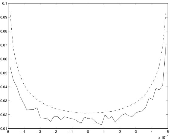
Figure 14: Fractional error in velocity for Poiseuille flow in a channel as a function of the transverse channel coordinate, $y$. The dashed line denotes the theoretical prediction including correlations and the solid line denotes DSMC simulation results.

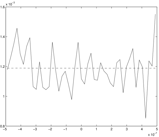
Figure 15: Fractional error in density for Poiseuille flow in a channel as a function of the transverse channel coordinate, $y$. The dashed line denotes the theoretical prediction including correlations and the solid line indicates DSMC simulation results.

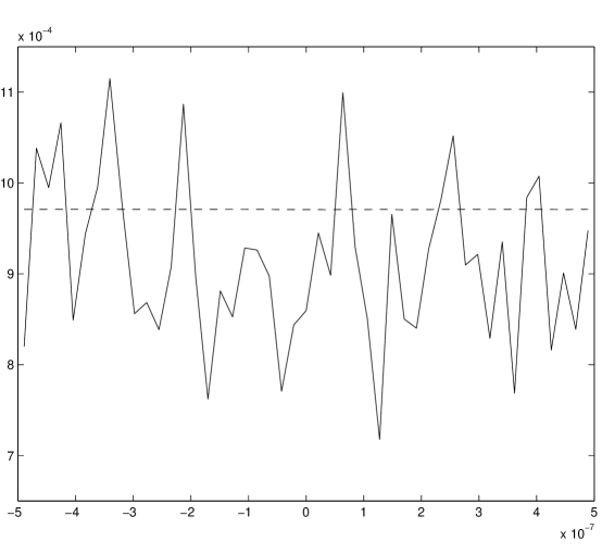
Figure 16: Fractional error in temperature for Poiseuille flow in a channel as a function of the transverse channel coordinate, $y$. The dashed line denotes the theoretical prediction including correlations and the solid line indicates DSMC simulation results.

In our DSMC simulations, the single-particle correlation coefficient for the velocity was estimated to be $\alpha_{c}\approx 0.94$ for $\Delta t=\lambda/(15c_{\mathrm{m}})$ by fitting Eq. (67) to data; the same value for $\alpha_{c}$ was found in both equilibrium and non-equilibrium simulations. In the comparison of figures 14, 15 and 16, however, we use $\alpha_{c}=1$ since mass, momentum and energy are conserved during collisions. We find that this analysis produces very good results in the case of density and temperature (see figures 15 and 16) and acceptable results for the case of mean velocity (see figure 14). Use of $\alpha_{c}=0.94$ would tend to make the agreement better but no theoretical justification exists for it. The value of $\alpha_{l}$ was directly calculated by assuming an equilibrium distribution. For our two-dimensional calculations with $\Delta x/(c_{\mathrm{m}}\Delta t)=2.5$, we find $\alpha_{l}\approx 0.6$. The effect of a mean flow is very small if the Mach number is small. This was verified through both direct evaluation of Eq. (70) using a local equilibrium distribution function and DSMC simulations.

5 Conclusions

We have presented expressions for the statistical error in estimating the velocity, density, temperature and pressure in molecular simulations. These expressions were validated for flow of a dilute gas and dense liquid in a two-dimensional channel using the direct simulation Monte Carlo and Molecular Dynamics respectively. Despite the non-equilibrium nature of the validation experiments, good agreement is found between theory and simulation, verifying that modifications to non-equilibrium results are very small. In particular, in the dense fluid case, despite the significant non-equilibrium due to a shear of the order of $5.5\times 10^{8}~{}\mathrm{s}^{-1}$, the agreement with equilibrium theory is remarkable. We thus expect these results to hold for general non-equilibrium applications of interest.

Predictions were also presented for the statistical error in estimating the shear stress and heat flux in dilute gases through cell averaging and surface averaging. Comparison with direct Monte Carlo simulations shows that the equilibrium assumption is justified. Within the same sets of assumptions, we were able to show that the distribution of particles leaving a cell is Poisson-distributed.

One consideration that significantly limits the applicability of cell (volume) averaging for transport quantities is their neglect of transport due to collisions in the cell volume. In DSMC in particular, as the time step of the simulation is increased, the fraction of particles in a cell undergoing collision increases, and as a result, the error from using the above method increases.

It was found that the fluctuation in state variables is significantly smaller compared to flux variables in the continuum regime $Kn\rightarrow 0$. This is important for the development of hybrid methods. Although a direct comparison was only presented between volume averaged quantities, we find that the fluxal measurements for the shear stress and heat flux perform similarly to the volume averaged counterparts (regarding scaling with the Knudsen number).

Appendix: Number Fluctuations in Dilute Gases

Consider an infinite ideal gas in equilibrium with mean number density, $n$. By definition, each infinitessimal volume element, $dV$, contains a particle with probability, $ndV$, and each such event in independent. From these assumptions, it is straightforward to show that the number of particles $N$ in an arbitrary volume $V$ is a Poisson random variable [12],

$$\mbox{Prob}(N=m)=\frac{e^{-\langle N\rangle}{\langle N\rangle}^{m}}{m!}$$

with mean and variance given by

$$\langle N\rangle=\langle\delta N^{2}\rangle=nV.$$

Note that this result does not strictly apply to a finite ideal gas because the probabilities of finding particles in different infinitessimal volumes are no longer independent, due to the global constraint of a fixed total number of particles. Nevertheless, it is an excellent approximation for most dilute gases, even finite non-ideal gases far from equilibrium (e.g. as demonstrated by simulations in the main text).

Now consider a property $A$ which each particle in a volume $V$ may possess independently with probability, $P_{A}$. In this Appendix, we show that the distribution of the number of such particles, $N_{A}$, is also a Poisson random variable with mean and variance given by

$$\langle N_{A}\rangle=\langle\delta N_{A}^{2}\rangle=P_{A}\langle N\rangle=P_{A}nV.$$

For example, in the main text we require the number of particles, $N_{ij}$, which travel from one region, $i$, to another region, $j$, in a time interval, $dt$. The proof given here, however, is much more general and applies to arbitrary number fluctuations of an infinite ideal gas in equilibrium, such as the number of particles in a certain region, moving in a certain direction, of a certain “color”, with speeds above a certain theshold, etc.

We begin by expressing $N_{A}$ as a random sum of random variables,

$$N_{A}=\sum^{N}_{i=1}\chi_{i}$$ (71)

where

$$\chi_{i}=\left\{\begin{array}[]{r@{\quad}l}1&\mathrm{if}\;A\;\mathrm{occurs}\\ 0&\mathrm{otherwise.}\end{array}\right.$$

is an indicator function for particle $i$ to possess property $A$, which is a Bernoulli random variable with mean, $P_{A}$. It is convenient to introduce probability generating functions,

$$f_{\chi}(z)=\sum^{\infty}_{m=0}\mbox{Prob}(\chi=m)z^{m}=(1-P_{A})+P_{A}z$$

and

$$f_{N}(z)=\sum^{\infty}_{m=0}\mbox{Prob}(N=m)z^{m}=\sum^{\infty}_{m=0}\frac{e^{-\langle N\rangle}{\langle N\rangle}^{m}z^{m}}{m!}=e^{\langle N\rangle(z-1)}$$ (72)

because the generating function for a random sum of random variables, as in Eq. (71), is simply given by a composition of the generating functions for the summand and the number of terms [12],

$$f_{N_{A}}(z)=\sum_{m=0}^{\infty}\mbox{Prob}(N_{A}=m)z^{m}=f_{N}\left(f_{\chi}(z)\right).$$

Combining these expressions we have

$$f_{N_{A}}(z)=e^{\langle N\rangle(1-P_{A}+P_{A}z-1)}=e^{P_{A}\langle N\rangle(z-1)}.$$

Comparing with Eq. (72) completes the proof that $N_{A}$ is a Poisson random variable with mean, $P_{A}\langle N\rangle$.

6 Acknowledgements

The authors wish to thank M. Malek-Mansour and B. Alder for helpful discussions. The authors would also like to thank X. Garaizar for making this work possible through the computer resources made available to them. This work was also supported, in part, by a grant from the University of Singapore, through the Singapore-MIT alliance.

References

- [1] Allen MP, Tildesley DJ. Computer Simulation of Liquids, Clarendon Press, Oxford, 1987.
- [2] D. Frenkel and B. Smit, “Understanding Molecular Simulation, From Algorithms to Applications”, Academic Press, San Diego, 2002.
- [3] Bird GA., 1994. Molecular Gas Dynamics and the Direct Simulation of Gas Flows, Clarendon Press, Oxford, 1994.
- [4] F. J. Alexander and A. L. Garcia, “The Direct Simulation Monte Carlo”, Computers in Physics, 11, 588-593, 1997.
- [5] M. Malek-Mansour, A. L. Garcia, G. C. Lie, E. Clementi, “Fluctuating Hydrodynamics in a Dilute Gas”, Physical Review Letters, 58, 874–877, 1987; A. L. Garcia, M. Malek-Mansour, G. Lie, M. Mareschal, E. Clementi, “Hydrodynamic fluctuations in a dilute gas under shear” Physical Review A, 36, 4348–4355, 1987.
- [6] Landau LD, Lifshitz EM. Statistical Mechanics. Oxford: Pergamon Press, 1980.
- [7] G. I. Taylor, “Diffusion by continuous movements”, Proc. London Math. Society, 20, 196–211, 1920.
- [8] F. Alexander, A. Garcia and B. Alder, “Cell Size Dependence of Transport Coefficients in Stochastic Particle Algorithms”, Phys. Fluids, 10 1540 (1998); Erratum: Phys. Fluids, 12 731 (2000).
- [9] N. G. Hadjiconstantinou, “Analysis of discretization in the direct simulation Monte Carlo”, Phys. Fluids, 12, 2634, 2000.
- [10] A. Garcia and W. Wagner, “Time step truncation error in direct simulation Monte Carlo”, Phys. Fluids, 12, 2621, 2000.
- [11] N. G. Hadjiconstantinou, “Hybrid Atomistic-Continuum Formulations and the Moving Contact-Line Problem”, Journal of Computational Physics, 154, 245–265 (1999).
- [12] W. Feller, An Introduction to Probability Theory and Its Applications, Vol 1, Chap. 12, 3rd edition, Wiley, 1968.
- [13] J. K. Johnson, J. A. Zollweg and K. E. Gubbins, “The Lennard-Jones equation of state revisited”, Molecular Physics, 78, 591–618, 1993.
- [14] A.L. Garcia, J.B. Bell, Wm.Y. Crutchfield, and B.J. Alder, “Adaptive Mesh and Algorithm Refinement using Direct Simulation Monte Carlo”, J. Comp. Phys. 154 134 (1999).
- [15] F. Alexander, A. Garcia and B. Alder, “A Consistent Boltzmann Algorithm”, Phys. Rev. Lett. 74 5212 (1995).
- [16] F. Alexander, A. Garcia and B. Alder, “The Consistent Boltzmann Algorithm for the van der Waals Equation of State”, Physica A 240 196 (1997).
- [17] L.D. Landau and E.M. Lifshitz, Statistical Mechanics, Part 2 (Pergamon Press, Oxford, 1980), Section 88.
- [18] L.D. Landau and E.M. Lifshitz, Statistical Mechanics, Part 1 (Pergamon Press, Oxford, 1980), Section 112.
- [19] P. Langevin, Comptes Ren. Acad. Sci. Paris 146, 530 (1908).
- [20] W. W. Liu and Y. C. Fang, “Implicit boundary conditions for direct simulation Monte Carlo method in MEMS flow predictions”, CMES, 1, 119, 2000.
- [21] G. H. Weiss, “Some applications of persistent random walks and the telegreapher’s equation,” in preparation.
- [22] R. Fürth,Schwankungeserscheinungen in der Physik (Sammlung Verlag, Braunschweig, 1920).
- [23] S. Ghosal and J. B. Keller, Nonlinearity 13, 1855 (2000).