Simulations of Helix Unwinding in Ferroelectric Liquid Crystals

Abstract

In bulk ferroelectric liquid crystals, the molecular director twists in a helix. In narrow cells, this helix can be unwound by an applied electric field or by boundary effects. To describe helix unwinding as a function of both electric field and boundary effects, we develop a mesoscale simulation model based on a continuum free energy discretized on a two-dimensional lattice. In these simulations, we determine both the director profile across the cell and the net electrostatic polarization. By varying the cell size, we show how boundary effects shift the critical field for helix unwinding and lower the saturation polarization. Our results are consistent with experimental data.

I Introduction

One of the most extensively studied phases of liquid crystals, both for basic research and for applications, is the smectic-C* (SmC*) phase of chiral molecules. In this phase, the molecules lie in layers and are tilted with respect to the layer normal direction. The combination of molecular chirality, smectic layering, and tilt order leads to two effects: a ferroelectric polarization within the smectic layer plane and a helical modulation in the orientation of the molecular tilt from layer to layer degennes93 . The ferroelectric polarization is useful for display devices, which use an applied electric field to switch the molecular orientation goodby91 . It is also useful for thermal sensors, which measure the temperature variation of the polarization, known as the pyroelectric effect osullivan95 ; crandall99 . Both of these applications require a uniform orientation of the molecules. Hence, the helix must be suppressed, or unwound, by an applied electric field or by boundary effects.

Helix unwinding has been modeled through continuum elastic theory. In a bulk SmC* phase, unwinding induced by an applied electric field can be described by the sine-Gordon equation, presented below meyer68 ; meyer69 ; kamien01 . Under an electric field, the helix distorts and the helical pitch increases. If the field is increased above a critical threshold, the pitch diverges and the helix is suppressed. By contrast, helix unwinding induced by boundary effects in a narrow cell is more complex cladis72 ; luban74 ; glogarova83 ; povse93 . In this case, a helix must have a series of disclination lines near the cell surfaces, which separate a twisted interior region from a uniform surface region. Continuum elastic theory shows that the unwinding transition is controlled by an energetic competition between the helical state with disclinations and the uniform untwisted state. If the cell thickness is below a critical threshold comparable to the helical pitch, the uniform state is favored and the helix is suppressed. (A third possible mechanism for helix unwinding is shear flow rey96 , but this is not often used in SmC* liquid crystals, and we will not discuss it here.)

In this paper, we investigate the unwinding of a SmC* helix by boundary effects, or by combined boundary and electric-field effects, through a series of Monte Carlo simulations of a continuum free energy discretized on a 2D lattice. These simulations serve two purposes. First, they allow us to visualize the complex director configuration within a narrow cell as a function of cell thickness and electric field. We obtain snapshots of the molecular tilt profile through the helix unwinding process. Second, they allow us to relate the microscopic director configuration to two macroscopic variables, an average chiral order parameter and the net electrostatic polarization of the cell. The latter variable can be compared with experimental measurements of SmC* cells.

In these simulations, we first consider boundary effects alone. We simulate the SmC* phase in narrow cells, and determine the structure of the helix as a function of cell thickness. We confirm that the helix unwinds at a threshold thickness approximately equal to the helical pitch, in agreement with continuum elastic theory. We then use the same Monte Carlo approach to simulate helix unwinding due to the combined effects of cell boundaries and electric field. In these simulations, we calculate both the molecular tilt profile across the cell and the net electrostatic polarization. We observe three distinct regimes of response, in which the helical pitch is first distorted and then expelled as the applied field is increased. By varying the cell thickness, we determine how boundary effects shift the critical field for helix unwinding and lower the saturation polarization. These simulation results are consistent with trends observed in experiments.

The plan of this paper is as follows. In Sec. II, we review the continuum elastic theory of the SmC* phase. We show how an applied electric field unwinds the SmC* helix in a bulk system, and sketch an approximate energetic argument for a finite cell. In Sec. III, we use Monte Carlo simulations to investigate the effects of finite cell thickness under zero applied electric field. In Sec. IV, we combine the effects of cell boundaries and applied electric field to determine the tilt profile and the polarization, and compare the polarization with experimental measurements.

II Theory

Figure 1: Idealized bookshelf geometry of a SmC* liquid crystal in a narrow cell. The helical axis is along the $z$-axis, perpendicular to the smectic layers. An electric field is applied along the $y$-axis.

A SmC* liquid crystal in a narrow cell has the idealized bookshelf geometry shown in Fig. 1. The molecules lie in layers, and they are tilted with respect to the smectic layer normal. The 3D orientation is represented by the director $\mathbf{n}$. This unit vector can be written in spherical coordinates as $\mathbf{n}=(\sin\theta\cos\phi,\sin\theta\sin\phi,\cos\theta)$, where $\theta$ is the polar angle of the tilt and $\phi$ is the azimuthal angle. The molecular tilt is conventionally described in terms of the projection of $\mathbf{n}$ into the layer plane, $\mathbf{c}=(\sin\theta\cos\phi,\sin\theta\sin\phi)$.

In this geometry, we expect the director to depend on the $y$ and $z$ coordinates. The $z$ coordinate is along the smectic layer normal. Because of the molecular chirality, the molecular orientation rotates in a helix from layer to layer, which makes the director a periodic function of $z$. The $y$ coordinate is the narrow dimension of the cell, with a thickness $d$ of order microns, across which an electric field $\mathbf{E}$ is applied. The molecules may interact strongly with the front and back surfaces of the cell, at $y=0$ and $d$. As a result, the director may rotate as a function of $y$. By contrast, we do not expect the director to depend on the third coordinate $x$. In this bookshelf geometry, the system is uniform as a function of $x$. (In certain liquid crystals, the smectic layers buckle as a function of $x$ crawford94 ; geer98 ; bartoli98 ; selinger00 , but we do not consider that effect here.) For that reason, we write the angles $\theta$ and $\phi$ as functions of $y$ and $z$.

We can now construct the simplest model free energy to describe variations in the director. This model must include four interactions. First, the smectic layer order interacts with the molecular orientation, and favors a particular tilt of the molecules with respect to the layers. This interaction can be expanded as a power series in the tilt magnitude $|\mathbf{c}|=\sin\theta$, which gives $-\frac{1}{2}r|\mathbf{c}|^{2}+\frac{1}{4}u|\mathbf{c}|^{4}$, for some series coefficients $r$ and $u$. In terms of these coefficients, the favored tilt is $|\mathbf{c}|=(r/u)^{1/2}$. Second, there is an electroclinic interaction of the molecules with the applied electric field $\mathbf{E}$. Because of the molecular chirality, this interaction couples the field in the $y$ direction with the tilt in the $x$ direction, so it can be written as $b\mathbf{z}\cdot\mathbf{E}\times\mathbf{c}=-bE_{y}c_{x}$. In other words, the electrostatic polarization is $\mathbf{P}=b\mathbf{z}\times\mathbf{c}$, or $P_{y}=-bc_{x}$. Third, there is a chiral interaction that favors a variation of the director from layer to layer, which can be written as $-\lambda\mathbf{z}\cdot\mathbf{c}\times\partial\mathbf{c}/\partial z$. Fourth, there is the Frank free energy for elastic distortions of the director, which limits the variations from layer to layer. This contribution can be written as $\frac{1}{2}K(\partial_{i}c_{j})(\partial_{i}c_{j})$, summed over $i$ and $j$. Putting these pieces together, the total free energy density becomes

$$F=-\frac{1}{2}r|\mathbf{c}|^{2}+\frac{1}{4}u|\mathbf{c}|^{4}+b\mathbf{z}\cdot\mathbf{E}\times\mathbf{c}-\lambda\mathbf{z}\cdot\mathbf{c}\times\frac{\partial\mathbf{c}}{\partial z}+\frac{1}{2}K(\partial_{i}c_{j})(\partial_{i}c_{j}).$$ (1)

This free energy is invariant under rotations in the $xy$ plane, but it is not invariant under reflections, because reflection symmetry is broken by the molecular chirality.

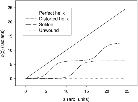
Figure 2: Unwinding of a SmC helix in a bulk system under an applied electric field $E$. Solid line: Perfect helix for $E=0$. Dashed line: Distorted helix under moderate $E$. Dot-dashed line: Single soliton in the director, near the threshold for helix unwinding. Dotted line: Unwound uniform director.

We can see immediately that this minimal model leads to a helix in the $z$ direction. Consider a director of the form $\mathbf{c}=(c\cos\phi,c\sin\phi)$, where the magnitude $c=\sin\theta$ is constant and the azimuthal angle $\phi$ depends on position. The free energy density simplifies to

$$F=-\frac{1}{2}rc^{2}+\frac{1}{4}uc^{4}-bEc\cos\phi-\lambda c^{2}\frac{\partial\phi}{\partial z}+\frac{1}{2}Kc^{2}\left|\nabla\phi\right|^{2}.$$ (2)

In the limit of zero electric field, $E=0$, we minimize this free energy over $\phi$ to obtain

$$\frac{\partial\phi}{\partial z}=\frac{\lambda}{K}.$$ (3)

Hence, the azimuthal angle increases linearly as $\phi(z)=\phi_{0}+q_{0}z$, with $q_{0}=\lambda/K$, as shown by the solid line in Fig. 2. This linear increase in $\phi$ implies a perfect sinusoidal helix in $\mathbf{c}$.

This minimal model also predicts unwinding of the helix under an applied electric field. This behavior is analogous to the theory of Meyer for a cholesteric phase in an electric or magnetic field meyer68 ; meyer69 ; kamien01 . For $E\not=0$, minimizing the free energy over $\phi$ gives

$$\frac{\partial^{2}\phi}{\partial z^{2}}=\frac{bE}{Kc}\sin\phi.$$ (4)

This is the standard sine-Gordon equation. The form of the solutions depends on the value of $E$, as shown in Fig. 2. For low $E$, the helix is distorted, so that the director is approximately aligned with the field in most of the system. As $E$ increases, the helix becomes even more distorted, with sharper steps between domains where $\phi$ is approximately a multiple of $2\pi$. Eventually the system crosses over into regime of uniform domains separated by sharp domain walls, or solitons. In that regime, a single soliton has the profile $\phi(z)=2\pi-4\tan^{-1}[\exp(-(z-z_{\rm wall})/\xi)]$, where $\xi=(2Kc/bE)^{1/2}$. As $E$ continues to increase, the spacing between the domain walls increases, or equivalently their density decreases. At the critical threshold $E=(\pi^{2}/8)(\lambda^{2}c/bK)$, the last domain wall vanishes and the system becomes uniform.

The question is now: What other types of influences can also unwind a SmC* helix? Clearly one possibility is surface effects. Interactions along the front and back surfaces of a finite cell, at $y=0$ and $d$, can anchor the director at those surfaces. If the elastic interactions described by the parameter $K$ are sufficiently strong, and the cell thickness $d$ is not too big, then this anchoring may extend throughout the interior of the cell, giving a uniform director. This is the basis of surface-stabilized ferroelectric liquid crystal cells goodby91 .

The threshold thickness for unwinding a helix is not obvious. As shown in Fig. 1, the helical pitch is along the $z$ direction, but the narrow dimension of the cell is along the $y$ direction. Because these directions are perpendicular, there is no simple geometric reason why a helix must unwind when the cell thickness is less than the pitch. Rather, there must be some energetic argument that relates these two length scales.

An energetic argument has been developed for narrow cells of the cholesteric phase cladis72 ; luban74 , and has been extended to narrow cells of the SmC* phase glogarova83 ; povse93 . In its simplest form, the argument can be stated as follows meyerprivate . If a cell has a helix in the interior, but a uniform director along the front and back surfaces, then it must have a series of disclination lines running along the $x$ direction near the surfaces. There must be one disclination line for each helical pitch. We can compare the energy of the helix (with disclinations) with the energy of the uniform state to find the threshold thickness for helix unwinding. The energy of the helix (with disclinations) is the negative energy gained from the helix plus the positive energy lost to the disclinations,

$$\frac{\Delta E}{\text{volume}}\approx-Kq_{0}^{2}+\frac{E_{\text{line}}}{(d)(\text{pitch})},$$ (5)

where $E_{\text{line}}$ is the disclination line energy per unit length. The helix unwinds if $\Delta E>0$, which implies

$$d\gtrsim\left(\frac{E_{\text{line}}}{K}\right)(\text{pitch}).$$ (6)

Since the line energy $E_{\text{line}}$ should be of order $K$, the threshold thickness should be comparable to the pitch.

In the following sections, we test this argument through a series of Monte Carlo simulations. In these simulations, we obtain snapshots of the director configuration for different cell thicknesses, both at zero field and under an applied electric field. These snapshots provide specific illustrations of the disclinations discussed above. For zero field, the simulations confirm that the helix unwinds at a critical thickness approximately equal to the helical pitch. For finite field, the simulations show helix unwinding induced by the combined effects of boundaries and electric field in a cell above the critical thickness. In both cases, we relate the microscopic snapshots of the director configuration to macroscopic variables. One of these variables, the net electrostatic polarization, can be compared with experimental measurements.

III Finite cells under zero electric field

To model helix unwinding in a finite cell of the SmC* phase, we map the system onto a 2D square lattice. The lattice dimensions represent the $yz$ plane shown in Fig. 1: $y$ is the narrow dimension of the cell and $z$ is the smectic layer normal. We assume the system is uniform in the $x$ direction. On each lattice site $(y,z)$ there is a 3D unit vector ${\mathbf{n}}(y,z)$ representing the local molecular director. This vector can be parametrized in terms of the polar angle $\theta(y,z)$ and azimuthal angle $\phi(y,z)$, or equivalently in terms of the projection ${\mathbf{c}}(y,z)$ into the smectic layer plane.

For the lattice simulations, we discretize the free energy of Eq. (1) to obtain

$$F =\sum_{(y,z)}\biggl{[}-\frac{1}{2}r|\mathbf{c}(y,z)|^{2}+\frac{1}{4}u|\mathbf{c}(y,z)|^{4}+b\mathbf{z}\cdot\mathbf{E}\times\mathbf{c}(y,z)$$

$$-\lambda\mathbf{z}\cdot\frac{\mathbf{c}(y,z)+\mathbf{c}(y,z+1)}{2}\times[\mathbf{c}(y,z+1)-\mathbf{c}(y,z)]$$

$$+\frac{1}{2}K(|\mathbf{c}(y+1,z)-\mathbf{c}(y,z)|^{2}+|\mathbf{c}(y,z+1)-\mathbf{c}(y,z)|^{2})\biggr{]},$$

with $\mathbf{E}=0$ in this section. This free energy is similar to the free energy studied in Ref. selinger00 but with one important difference: that paper simulated the $xy$ plane, but we now simulate the $yz$ plane.

A further consideration for the simulations is boundary conditions. Experimental cells may be symmetric, with the local director aligned along the same direction on both front and back confining walls, or they may be asymmetric, with the director aligned along one wall and an open boundary on the other side. In our simulations we use an aligning boundary condition with the director fixed on the wall at $y=0$ with a specified tilt angle. On the other wall at $y=d$ we use the boundary condition $\partial c(y,z)/\partial y=0$. This arrangement can represent an asymmetric cell, or one half of a symmetric cell, with the other half a mirror image of the first. Experimental cells are very large in the $z$ direction so that the top and bottom boundaries should not affect the physics of the interior. In the simulations, we use the boundary condition $\partial c(y,z)/\partial z=0$ for the top and bottom boundaries.

We simulate the system with the parameters $r=0.007596$, $u=1$, $b=1$, $E=0$, $K=1.5$, and $\lambda=0.25$ and $0.125$. The small value of $r$ corresponds to a tilt angle of approximately $5^{\circ}$. We use the large $z$ dimension of 160, and several values of the thickness $d$ in the $y$ direction. For each set of parameters and system size, we begin the simulations in a disordered state at a high Monte Carlo temperature, and then slowly reduce the temperature until the system settles into a single ground state and the fluctuations in $\mathbf{c}$ become negligible. This procedure can be regarded as a simulated-annealing minimization of the lattice free energy of Eq. (III).

(a) (b)

Figure 3: Director configuration in the $yz$ plane for simulations with $\lambda=0.25$, leading to a pitch of approximately 38. The system has an aligning boundary along the left side ($y=0$). Note that the $y$ axis is exaggerated compared with the $z$ axis. (a) For a thickness of 10 ($y=0$ through $9$), the system is uniform, except for some edge effects at the top and bottom. (b) For a thickness of 12, the system has a clear helix.

(a)

(b)

Figure 4: Director configuration in the $yz$ plane for simulations with $\lambda=0.125$, leading to a pitch of approximately 75. (a) For a thickness of 23, the system is uniform, except for some edge effects. (b) For a thickness of 25, there is a clear helix.

To visualize the simulation results, we draw the $yz$ plane in Figs. 3 and 4. The director configuration is represented by short lines that show the projection of the 3D director into the $yz$ plane. Hence, vertical lines indicate $c_{y}=0$, and tilted lines indicate $c_{y}\not=0$. Because the lines representing the director are drawn close together, helical regions resemble twisted ribbons.

Figure 3 shows the simulation results for $\lambda=0.25$ and $K=1.5$. For these parameters, the favored wavevector is $q_{0}=\lambda/K\approx 0.17$, and hence the unperturbed pitch is $2\pi/q_{0}\approx 38$. For a thickness of 10, the system is uniform, with $c_{y}=0$ everywhere except near the top and bottom surfaces. Those distortions are edge effects within a fractional pitch of the free surfaces, which do not affect the bulk behavior inside the cell. Hence, we see that the system of thickness 10 is unwound. By contrast, for a thickness of 12, the system shows a well-defined helix, with a periodic modulation of $c_{y}$ throughout the cell, except very close to the aligning surface at $y=0$. Thus, there is a clear helix winding/unwinding transition as a function of thickness. The transition occurs at a critical thickness between 10 and 12 for a cell with asymmetric boundary conditions (or a half-thickness between 10 and 12 if the simulation is regarded as half of a symmetric cell). This critical thickness is not equal to the pitch, but it is certainly the same order of magnitude, in agreement with the theoretical expectation of Eq. (6).

Figure 4 shows the corresponding results for $\lambda=0.125$. In this case, the favored wavevector is $q_{0}\approx 0.083$, so the unperturbed pitch is $2\pi/q_{0}\approx 75$. For a thickness of 23, the system is uniform, again except for some edge effects near the top and bottom surfaces. By comparison, for a thickness of 25, there is a distinct helix throughout the interior of the cell. Thus, there is a helix winding/unwinding transition with a critical thickness between 23 and 25. This critical thickness is approximately twice the critical thickness of the previous case. Hence, we see that the critical thickness is approximately proportional to the pitch, again in agreement with the theoretical expectation.

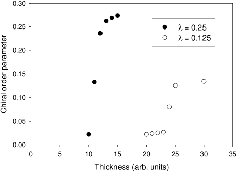
Figure 5: The chiral order parameter $\chi$ defined in Eq. (8), as a function of the system thickness $d$. For $\lambda=0.25$ (pitch $\approx 38$), the unwinding transition occurs at a thickness between 10 and 12. For $\lambda=0.125$ (pitch $\approx 75$), the transition occurs at a thickness between 23 and 25.

For a quantitative measurement of helix winding and unwinding, we must define a chiral order parameter. One simple choice of a chiral order parameter is just the chiral term of the free energy (III), without the factor of $\lambda$ itself,

$$\chi = -\frac{1}{N_{\text{sites}}}\sum_{(y,z)}\mathbf{z}\cdot\frac{\mathbf{c}(y,z)+\mathbf{c}(y,z+1)}{2}$$ (8)

$$\phantom{-\frac{1}{N_{\text{sites}}}\sum_{(y,z)}}\times[\mathbf{c}(y,z+1)-\mathbf{c}(y,z)].$$

Figure 5 shows this order parameter as a function of the system thickness $d$ for both series of simulations, with $\lambda=0.25$ and $0.125$. For $\lambda=0.25$, the plot shows a sharp transition between thickness 10 and 12, as $\chi$ jumps from 0.022 to 0.24. For $\lambda=0.125$, there is a distinct transition between thickness 23 and 25, as $\chi$ jumps from 0.026 to 0.13. This analysis confirms that the winding/unwinding transition occurs at a thickness that is proportional to, and the same order of magnitude as, the helical pitch.

IV Finite cells under an electric field

In the previous section, we showed that a SmC* helix can be unwound by surface effects in a finite cell. If the thickness is greater than the critical threshold, the helix is present at zero electric field. However, when an electric field is applied, the helix can be unwound by the combined effects of the surfaces and the electric field. In this section, we simulate that combination of surface and field effects.

For these simulations, we use the same Monte Carlo approach as in the previous section. We use the discretized free energy of Eq. (III) with the parameters $r=0.0625$, $u=1$, $b=1$, $K=1.5$, and $\lambda=0.25$. This value of $r$ corresponds to a tilt angle of approximately $15^{\circ}$. We perform the simulations for four values of the cell thickness, $d=10$, 20, 40, and 60, and scan through the electric field $E$ at each thickness. For these parameters, the unperturbed pitch is $2\pi K/\lambda\approx 38$ and hence, based on the results of the previous section, the zero-field winding/unwinding transition occurs at a thickness between 10 and 12. Hence, the simulations at thickness $10$ should be unwound at all values of the electric field, while the simulations at larger thickness should go through the winding/unwinding transition as a function of electric field.

(a) (b)

(c) (d)

Figure 6: Director configuration in the $yz$ plane as a function of increasing electric field, for a fixed thickness of 20. (a) $E=0$. (b) $E=0.004$. (c) $E=0.006$. (d) $E=0.008$.

Figure 6 shows the simulation results for the system of thickness 20. For $E=0$, the system has a helix everywhere in the cell, except a narrow region near the aligning boundary at $y=0$. By comparison, for $E=0.004$, the helix is suppressed in much of the cell. It persists only in regions of the cell near the free surfaces at the top and bottom. This behavior near the free surfaces is consistent with the previous section, which showed that free surfaces tend to favor the helical modulation. When the field increases to $E=0.006$, the helix is suppressed in more of the cell, and it persists only in smaller regions near the top and bottom surfaces. Once the field reaches $E=0.008$, the helix is suppressed throughout the interior of the cell. The director in the cell is now uniform, except for very narrow edge effects at the top and bottom. Hence, the electric field has driven the finite cell through the helix winding/unwinding transition.

As in the previous section, we need an order parameter to describe the winding/unwinding transition quantitatively. In this case, the electrostatic polarization provides an experimentally relevant order parameter, which shows how the net polar order of the cell couples to the electric field. As argued in Sec. II, the polarization is the quantity conjugate to the electric field in the free energy, and hence $\mathbf{P}=b\mathbf{z}\times\mathbf{c}$, or $P_{y}=-bc_{x}$. We average this quantity over the cell to obtain

$$P_{y}=-\frac{1}{N_{\text{sites}}}\sum_{(y,z)}bc_{x}(y,z).$$ (9)

Figure 7 shows the simulation results for the polarization as a function of electric field for each cell thickness. Figure 7(a) presents the results on a linear scale, and Fig. 7(b) presents the same results on a logarithmic scale. Note that the polarization is not zero at zero field because of the symmetry-breaking surface alignment at $y=0$.

(a)

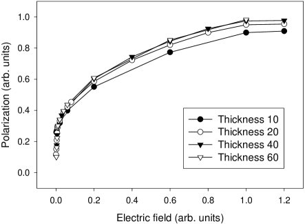
(b)

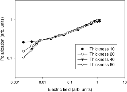
Figure 7: Simulation results for the polarization as a function of electric field in cells of four thicknesses. (a) Linear scale. (b) Logarithmic scale. On the logarithmic scale, note the three regimes of helix unwinding, suppressed twist, and saturation.

From the plots in Fig. 7, we can see that the system has three distinct regimes in its response to an electric field. For low field $E\lesssim 0.01$, there is a regime of helix unwinding. In this regime, an increasing electric field gradually aligns the directors, suppresses the helix, and prevents the local polarization from averaging to zero. As a result, the net polarization increases rapidly as a function of field. (This low-field regime does not occur for the lowest thickness $d=10$, because the helix is suppressed by surface effects even without a field.) For intermediate field $0.01\lesssim E\lesssim 1$, there is a regime of suppressed twist. In this regime, the helix is already unwound, so the only effect of electric field is to increase the local tilt and polarization. Hence, the net polarization increases more slowly, roughly as $E^{1/3}$. Finally, for high field $E\gtrsim 1$, there is a saturated regime. Here, the helix is already unwound, the local tilt is at its maximum value $c_{x}=1$, and the polarization is at its maximum value of $P_{y}=b$. Although the simulations only go to $E=1.2$, we see that the polarization cannot increase at higher field because it is already saturated.

In Fig. 7, we can also compare the relative polarization of thinner and thicker cells. For low field, thinner cells have a higher polarization than thicker cells, because the helix reduces the polarization in thicker cells but the aligning boundary at $y=0$ unwinds the helix in thinner cells. By contrast, for high field, thicker cells have a higher polarization than thinner cells, because there is no helix at any thickness, and surface effects at $y=d$ suppress the polarization in thinner cells. A similar high-field limit has been discussed by Shenoy et al. shenoy01 , who see the same effect experimentally in cells with different boundary conditions. For intermediate field, the polarization of thinner and thicker cells must cross.

To compare our results with experimental measurements of the polarization as a function of electric field, we must take into account one subtlety of the experiments. As shown by Ruth et al. ruth94 ; hermann96 , the polarization observed experimentally (by the triangle-wave technique or other techniques) is not the total polarization conjugate to the electric field. Rather, it is a specific nonlinear component of the polarization, which can be written as

$$P_{\text{obs}}(E)=P(E)-E\left(\frac{dP}{dE}\right).$$ (10)

The difference between the total polarization $P(E)$ and the observable polarization $P_{\text{obs}}(E)$ is small when $P(E)$ is saturated, but it is significant whenever $P(E)$ varies with $E$. Hence, we must extract $P_{\text{obs}}(E)$ from the simulations and compare that quantity with experiments.

To extract $P_{\text{obs}}(E)$ from the simulations, we need to calculate the derivative $dP/dE$. For that reason, we fit the simulation results for the polarization to the function $P(E)=(1+\alpha E)/(\beta+\gamma E)$. This is just an empirical fitting function, with no theoretical basis, but it gives a fairly good fit to the data in Fig. 7(a). We can then differentiate this function and calculate the observable polarization $P_{\text{obs}}(E)$ that corresponds to the simulation results.

(a)

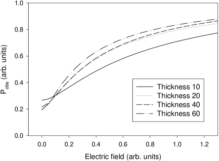
(b)

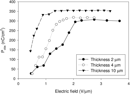
Figure 8: (a) Simulation results for the observable polarization $P_{\text{obs}}=P-E(dP/dE)$ in cells of four thicknesses. (b) Experimental data for $P_{\text{obs}}$ in three cells crandallprivate .

Figure 8(a) shows the results for $P_{\text{obs}}(E)$ extracted from the simulations at each system size. This function is small for low $E$, then increases towards its saturation level $P_{\text{obs}}=b$ at high $E$. As discussed above, thinner cells have a higher value of $P_{\text{obs}}$ at low field, and thicker cells have a higher value of $P_{\text{obs}}$ at high field. By comparison, Fig. 8(b) shows sample experimental measurements of $P_{\text{obs}}$ as a function of applied electric field in three cells with asymmetric boundary conditions crandallprivate . The material is 10PPBN4 (described in Ref. naciri95 ), and the temperature is 7 ^∘C below the SmA-SmC transition. Note that the experimental data show the same general features as the theoretical plots. In particular, we see the same crossover between higher $P_{\text{obs}}$ in thinner cells at low field and higher $P_{\text{obs}}$ in thicker cells at high field. Thus, the simulation results are consistent with the trends seen in experiments.

In conclusion, we have developed an approach for simulating the helix winding/unwinding transition in SmC* liquid crystals. This approach is based on a minimal model for the free energy, which includes a chiral term that favors a helical modulation of the director from layer to layer. This bulk free energy competes with surface effects and electric-field effects, which both favor a uniform alignment of the director. In zero field, the competition between the bulk helix and the surface alignment leads to helix unwinding at a critical thickness approximately equal to the helical pitch. When an electric field is applied, the field-induced alignment adds to the surface effects, and induces helix unwinding even for thicker cells. The electrostatic polarization is an appropriate order parameter to quantify this field-induced unwinding, and our simulation results for the polarization are consistent with experimental measurements.

- (1) P. G. de Gennes and J. Prost, The Physics of Liquid Crystals, 2nd edition (Oxford, Oxford University Press, 1993).
- (2) J. W. Goodby, R. Blinc, N. A. Clark, S. T. Lagerwall, M. A. Osipov, S. A. Pikin, T. Sakurai, K. Yoshino, and B. Žekš, Ferroelectric Liquid Crystals: Principles, Properties and Applications (Gordon and Breach, Amsterdam, 1991).
- (3) J. W. O’Sullivan, Yu. P. Panarin, and J. K. Vij, J. Appl. Phys. 77, 1201 (1995).
- (4) K. Crandall, D. Shenoy, S. Gray, J. Naciri, and R. Shashidhar, Proc. IRIA-MSS on Infrared Materials, p. 173 (1999).
- (5) R. B. Meyer, Appl. Phys. Lett. 12, 281 (1968)
- (6) R. B. Meyer, Appl. Phys. Lett. 14, 208 (1969).
- (7) R. D. Kamien and J. V. Selinger, J. Phys.: Condens. Matter 13, R1 (2001).
- (8) P. E. Cladis and M. Kléman, Mol. Cryst. Liq. Cryst. 16, 1 (1972).
- (9) M. Luban, D. Mukamel, and S. Shtrikman, Phys. Rev. A 10, 360 (1974).
- (10) M. Glogarová, L. Lejček, J. Pavel, V. Janovec, and J. Fousek, Mol. Cryst. Liq. Cryst. 91, 309 (1983).
- (11) T. Povše, I. Muševič, B. Žekš, and R. Blinc, Liq. Cryst. 14, 1587 (1993).
- (12) A. D. Rey, Phys. Rev. E 53, 4198 (1996).
- (13) G. P. Crawford, R. E. Geer, J. Naciri, R. Shashidhar, and B. R. Ratna, Appl. Phys. Lett. 65, 2937 (1994).
- (14) R. E. Geer, S. J. Singer, J. V. Selinger, B. R. Ratna, and R. Shashidhar, Phys. Rev. E 57, 3059 (1998).
- (15) F. J. Bartoli, J. R. Lindle, S. R. Flom, R. Shashidhar, G. Rubin, J. V. Selinger, and B. R. Ratna, Phys. Rev. E 58, 5990 (1998).
- (16) J. V. Selinger, J. Xu, R. L. B. Selinger, B. R. Ratna, and R. Shashidhar, Phys. Rev. E 62, 666 (2000).
- (17) R. B. Meyer, private communication.
- (18) D. Shenoy, A. Lavarello, J. Naciri, and R. Shashidhar, Liq. Cryst. 28, 841 (2001).
- (19) J. Ruth, J. V. Selinger, and R. Shashidhar, Appl. Phys. Lett. 65, 1590 (1994).
- (20) D. Hermann, L. Komitov, S. T. Lagerwall, G. Andersson, R. Shashidhar, J. V. Selinger, and F. Giesselmann, Ferroelectrics 181, 371 (1996).
- (21) K. A. Crandall, private communication.
- (22) J. Naciri, B. R. Ratna, S. Baral-Tosh, P. Keller, and R. Shashidhar, Macromolecules 28, 5274 (1995).