Gain in quantum cascade lasers and superlattices: A quantum transport theory

Abstract

Gain in current-driven semiconductor heterostructure devices is calculated within the theory of nonequilibrium Green functions. In order to treat the nonequilibrium distribution self-consistently the full two-time structure of the theory is employed without relying on any sort of Kadanoff-Baym Ansatz. The results are independent of the choice of the electromagnetic field if the variation of the self-energy is taken into account. Excellent quantitative agreement is obtained with the experimental gain spectrum of a quantum cascade laser. Calculations for semiconductor superlattices show that the simple 2-time miniband transport model gives reliable results for large miniband widths at room temperature.

I Introduction

The prospect of a semiconductor laser in the infrared and THz region has been one of the key reasons for the development and study of semiconductor heterostructure elements, since the first proposal of semiconductor superlattices in 1970 Esaki and Tsu (1970). A possible gain mechanism may be based on two different ideas: (i) At certain electrical fields resonant tunneling between different subbands can lead to population inversion associated with gain at the transition energy Kazarinov and Suris (1971). This idea was realized in the quantum cascade laser Faist et al. (1994), which has become an important device in the infrared region. Lasing in the THz region has been demonstrated very recently as well Köhler et al. (2002). For further details, see the review Gmachl et al. (2001). (ii) The occurrence of negative differential conductivity in superlattices gives raise to gain in the low frequency range extending up to frequencies of the order of the Bloch frequency Ktitorov et al. (1972). Despite a strong effort by several groups all over the world, this idea is still not realized. The difficulty in its realization is attributed to the instability of the operating state leading to domain formation Renk et al. (1998), which may be circumvented by different strategies Wacker et al. (1997); Kroemer (2000); Allen et al. (1991). For further references and a detailed discussion see Ref. Wacker, 2002.

These concepts for gain are commonly described in different ways: (i) An external electromagnetic field causes transitions between different levels, where the transition rate $R$ is evaluated by Fermi’s golden rule. If stimulated emission dominates stimulated absorption (i.e., for population inversion), gain occurs at the transition frequency. For a pair of states $\alpha,\beta$ with energies $E_{\alpha},E_{\beta}$, occupation probabilities $f_{\alpha},f_{\beta}$, and a dipole matrix element $z_{\alpha\beta}$, the contribution to the material gain (i.e., increase of light intensity per length) is given by

$$\begin{split}G_{m}(\omega)=&\frac{1}{V}\frac{R^{\text{stim. em.}}_{\alpha\to\beta}-R^{\text{stim. abs.}}_{\beta\to\alpha}}{\mbox{Photon flux per area}}\\ =&\frac{\pi\omega\left|ez_{\alpha\beta}\right|^{2}}{\sqrt{\epsilon_{r}}c\epsilon_{0}V}\delta(E_{\alpha}-E_{\beta}-\hbar\omega)(f_{\alpha}-f_{\beta})\,,\end{split}$$ (1)

where $V$ is the normalization volume, $e<0$ is the electron charge, $c$ is the vacuum speed of light, and $\epsilon_{r}$ the background dielectric constant.

(ii) Transport theory in the presence of alternating electric fields provides the complex dynamical conductance $\sigma(\omega)$. Standard electrodynamics (see, e.g., section 7.5 of Ref. Jackson (1998)) gives the material gain (the negative absorption coefficient $\alpha$, which is assumed to be small compared to the wave vector here)

$$G_{m}(\omega)\approx-\frac{\Re\{\sigma(\omega)\}}{c\epsilon_{0}\sqrt{\epsilon_{r}-\Im\{\sigma(\omega)\}/\epsilon_{0}\omega}}\,.$$ (2)

Thus, gain is equivalent to a negative differential conductivity in the respective frequency range. This concept has been frequently applied to superlattice transport. (For superlattices Eq. (1) gives zero gain in the basis of Wannier Stark states, as the translational symmetry gives identical $f_{\alpha}$ for all Wannier-Stark levels.) Here the current is either evaluated from a semiclassical miniband transport model Ktitorov et al. (1972); Renk et al. (1998); Kroemer (2000); Allen et al. (1991) or by sequential tunneling between different layers Tucker and Feldman (1985); Wacker et al. (1997); Platero and Aguado (1997). While these approaches use a macroscopic current density in Eq. (2), the consideration of polarization currents allows for a derivation of Eq. (1), see, e.g., Ref. Haug and Koch, 1994.

For complicated semiconductor heterostructures, with a variety of different tunneling and optical transitions, gain may result both from optical transitions in the spirit of (i) and macroscopic currents in the spirit of (ii). The aim of this paper is to show the feasibility of a general approach based on a quantum transport theory which treats both mechanisms on a equal footing.

The method of nonequilibrium Green functions Kadanoff and Baym (1962) is used here, which has been frequently applied to light emission in semiconductors (see, e.g., Refs. Schmitt-Rink et al., 1988; Haug and Jauho, 1996; Henneberger and Koch, 1996; Pereira, Jr. and Henneberger, 1998 and references given therein). While these works consider transitions between the conduction and valence band, the focus in this paper is on transitions within the conduction band in current-driven heterostructure devices. The calculations are performed in two steps: First the transport problem is solved by evaluating a self-consistent stationary solution of the quantum kinetic equations for a given applied bias. This provides us with the Green functions describing the electronic state far from equilibrium. In a second step, an additional weak radiation field is taken into account. The time-dependent kinetic equations are linearized around the stationary nonequilibrium state in oder to study the linear response of the current-driven system. The formulation used here employs the full two-time structure of the theory without any sort of (generalized) Kadanoff-Baym ansatz Lipavský et al. (1986). The capability of the approach is demonstrated by calculations of the gain spectra in a quantum cascade laser and a superlattice.

II Theory

We describe a general system by a set of orthonormal states labeled $\alpha$ with energies $E_{\alpha}$ and write the Hamiltonian in the form:

$$\hat{H}=\sum_{\alpha}E_{\alpha}\hat{a}^{{\dagger}}_{\alpha}\hat{a}_{\alpha}+\sum_{\alpha\beta}U_{\alpha\beta}(t)\hat{a}^{{\dagger}}_{\alpha}\hat{a}_{\beta}+\hat{H}_{\textrm{scatt}}$$ (3)

where $\hat{a}_{\alpha}$ and $\hat{a}^{{\dagger}}_{\alpha}$ are electron annihilation and creation operators in the state $\alpha$. $U_{\alpha\beta}(t)$ represents the matrix elements of the kinetic energy and the potential part of the Hamiltonian $\hat{H}$. In the following, $U(t)$ will be split into a constant part $\tilde{U}$ and a small time-dependent perturbation $\delta{U}(t)$ describing the interaction with a radiation field. Finally, $\hat{H}_{\textrm{scatt}}$ contains the part of the Hamiltonian which will be solved perturbatively (such as impurity, phonon, or electron-electron scattering matrix elements).

Within the theory of nonequilibrium Green functions Kadanoff and Baym (1962); Haug and Jauho (1996) the key quantities are the correlation function (or ’lesser’ Green function)

$$\begin{split}G^{<}_{\alpha_{1},\alpha_{2}}(t_{1},t_{2})={\rm i}\Big{\langle}\hat{a}^{{\dagger}}_{\alpha_{2}}(t_{2})\hat{a}_{\alpha_{1}}(t_{1})\Big{\rangle}\end{split}$$ (4)

and the retarded/advanced Green functions

$$\begin{split}G^{\text{ret/adv}}_{\alpha_{1},\alpha_{2}}&(t_{1},t_{2})=\mp{\rm i}\Theta[\pm(t_{1}-t_{2})]\\ &\times\Big{\langle}\hat{a}_{\alpha_{1}}(t_{1})\hat{a}^{{\dagger}}_{\alpha_{2}}(t_{2})+\hat{a}^{{\dagger}}_{\alpha_{2}}(t_{2})\hat{a}_{\alpha_{1}}(t_{1})\Big{\rangle}\,,\end{split}$$ (5)

respectively, where the Heisenberg picture is used.

First consider a stationary state with a time independent matrix $U(t)=\tilde{U}$, neglecting the radiation field. In this case all functions depend only on the time difference $t_{1}-t_{2}$ [these stationary state functions are labeled by a tilde, e.g., $\tilde{G}(t_{1}-t_{2})$, in the following], and it is convenient to work in Fourier space defined by

$$\tilde{G}_{\alpha_{1},\alpha_{2}}(E)=\frac{1}{\hbar}\int{\rm d}t\,{\rm e}^{{\rm i}Et/\hbar}\tilde{G}_{\alpha_{1},\alpha_{2}}(t)\,.$$ (6)

Then Eqs. (24,25) of the appendix become the matrix equations

$$\begin{split}\left(E-E_{\alpha_{1}}\right)\tilde{G}^{\rm ret}_{\alpha_{1},\alpha_{2}}(E)-\sum_{\beta}\tilde{U}_{\alpha_{1},\beta}\ \tilde{G}^{\rm ret}_{\beta,\alpha_{2}}(E)\\ =\delta_{\alpha_{1},\alpha_{2}}+\sum_{\beta}\tilde{\Sigma}^{\rm ret}_{\alpha_{1},\beta}(E)\tilde{G}^{\rm ret}_{\beta,\alpha_{2}}(E)\end{split}$$ (7)

$$\tilde{G}^{<}_{\alpha_{1},\alpha_{2}}(E)=\sum_{\beta,\beta^{\prime}}\tilde{G}^{\rm ret}_{\alpha_{1},\beta}(E)\tilde{\Sigma}^{<}_{\beta,\beta^{\prime}}(E)\tilde{G}^{\rm adv}_{\beta^{\prime},\alpha_{2}}(E)\,.$$ (8)

These have to be solved self-consistently together with the equations for the self-energies which are functionals of the Green functions

$$\tilde{\Sigma}(E)={\cal F}_{E}\left\{\tilde{G}^{\textrm{ret}}(E^{\prime}),\tilde{G}^{<}(E^{\prime})\right\}\,.$$ (9)

This standard approach allows for a self-consistent evaluation of the Green functions $\tilde{G}$ in a nonequilibrium situation caused by an applied bias (contained in $\tilde{U}$). Details, such as the specific form of the functionals in the self-consistent Born approximation, can be found in, e.g., Datta (1995); Lake et al. (1997); Wacker (2002).

The current density (in the $z$-direction) can be evaluated from the expectation value of the momentum operator divided by the mass:

$$\begin{split}J_{z}=&\frac{e}{V}\langle\frac{\hat{p}_{z}}{m}\rangle=\frac{e}{V}\frac{{\rm i}}{\hbar}\langle[\hat{H},\hat{z}]\rangle\\ =&\frac{e}{\hbar V}\sum_{\alpha\beta}W_{\alpha\beta}G^{<}_{\beta\alpha}(t,t)+\mbox{Scattering currents}\end{split}$$ (10)

where $W_{\alpha\beta}=\sum_{\gamma}(U_{\alpha\gamma}z_{\gamma\beta}-z_{\alpha\gamma}U_{\gamma\beta})$. The scattering currents result from the scattering part of the Hamiltonian and can be expressed in terms of self-energies. Details will be given elsewhere.

Now we consider the influence of an additional time-dependent potential

$$\delta{\bf U}(t)=\int\frac{{\rm d}\omega}{2\pi}\delta{\bf U}(\omega){\rm e}^{-{\rm i}\omega t}$$ (11)

in the Hamiltonian. (Bold capital symbols denote matrices in the state indices $\alpha,\beta$). We treat the change of the system in linear response, and set

$$G(t_{1},t_{2})=\tilde{G}(t_{1}-t_{2})+\delta G(t_{1},t_{2})\,.$$ (12)

The chance in the self-energies is described within the linearization of the functional (here in the time domain)

$$\Sigma(t_{1},t_{2})={\cal F}_{t}\left\{\tilde{G}+\delta G\right\}\approx\tilde{\Sigma}(t_{1}-t_{2})+\delta\Sigma(t_{1},t_{2})\,.$$ (13)

Such a decomposition has been used in Ref. Schmitt-Rink et al., 1988 for Hartree-Fock self-energies, e.g.. In this case, the time-dependence of the self-energies allows for a reduction to density matrix equations by setting $t_{1}=t_{2}$. In contrast, in our case, where scattering effects are considered, $\delta G$ exhibits an explicit time dependence in both arguments. This two time structure is fully taken into account here. Therefore we apply the Fourier decomposition in both times via

$$\delta{\bf G}(t_{1},t_{2})=\int\frac{{\rm d}\omega}{2\pi}{\rm e}^{-{\rm i}\omega t_{1}}\int\frac{{\rm d}E}{2\pi}\delta{\bf G}(\omega,E){\rm e}^{-{\rm i}E(t_{1}-t_{2})/\hbar}$$ (14)

The same decomposition is used for $\delta\Sigma$. It is shown in appendix C that $\delta G$ is determined within linear response by the following equations:

$$\delta{\bf G}^{\text{ret/adv}}(\omega,E) = \tilde{\bf G}^{\text{ret/adv}}(E+\hbar\omega)\left[\delta{\bf U}(\omega)+\delta\bm{\Sigma}^{\text{ret/adv}}(\omega,E)\right]\tilde{\bf G}^{\text{ret/adv}}(E)$$ (15)

$$\delta{\bf G}^{<}(\omega,E) = \tilde{\bf G}^{\text{ret}}(E+\hbar\omega)\delta{\bf U}(\omega)\tilde{\bf G}^{<}(E)+\tilde{\bf G}^{<}(E+\hbar\omega)\delta{\bf U}(\omega)\tilde{\bf G}^{\text{adv}}(E)$$ (16)

$$+ \tilde{\bf G}^{\text{ret}}(E+\hbar\omega)\delta\bm{\Sigma}^{\text{ret}}(\omega,E)\tilde{\bf G}^{<}(E)+\tilde{\bf G}^{\text{ret}}(E+\hbar\omega)\delta\bm{\Sigma}^{<}(\omega,E)\tilde{\bf G}^{\text{adv}}(E)$$

$$+ \tilde{\bf G}^{<}(E+\hbar\omega)\delta\bm{\Sigma}^{\text{adv}}(\omega,E)\tilde{\bf G}^{\text{adv}}(E)$$

The changes in self-energy $\delta\Sigma$ are functionals of $\delta G$, which have to be evaluated self-consistently with $\delta G$. The derivation of the functionals from the linearization of Eq. (13) is straightforward and can be performed for arbitrary self-energies. The situation is particularly simple for the self-consistent Born approximation, where the functional ${\cal F}$ is linear in $G$, and one finds: $\delta\Sigma(\omega,E)={\cal F}_{E}\left\{\delta G^{\textrm{ret}}(\omega,E^{\prime}),\delta G^{<}(\omega,E^{\prime})\right\}$ with the same functional as Eq. (9). (Note, that $\delta{\bf G}^{\mathrm{adv}}(\omega,E^{\prime})=\left[\delta{\bf G}^{\mathrm{ret}}(\omega,E^{\prime})\right]^{{\dagger}}$ does not hold for the time-dependent quantities. Thus, the advanced quantities should be calculated explicitely)

The terms related to $\delta\bm{\Sigma}$ correspond to the ladder corrections in the evaluation of diagrams for the Kubo formula in equilibrium. It is a general advantage of linear response within nonequilibrium Green functions that these terms are obtained directly, see also Haug and Jauho (1996); Wacker and Hu (1999).

Now we consider the linear response to an external radiation field where the electric field points in the $z$ direction. This gives additional terms in the Hamiltonian $\hat{H}=(\hat{\vec{p}}-e\vec{A})^{2}/2m+V(\vec{r})+e\varphi(\vec{r})$, where $\vec{A},\varphi$ are the electromagnetic potentials. Neglecting quadratic terms in the radiation field and terms containing $k$ (i.e., assuming that the wavelength is large compared to the size of the active region), the following perturbation potentials are obtained (see Appendix D): In the Coulomb gauge

$$\delta U_{\alpha,\beta}(\omega)=\frac{e}{{\rm i}\omega}F(\omega)\left(\frac{\hat{p}_{z}}{m}\right)_{\alpha,\beta}\approx-\frac{eF(\omega)}{\hbar\omega}W_{\alpha,\beta}$$ (17)

neglecting the scattering part of $\hat{H}$; in the Lorentz gauge

$$\delta U_{\alpha,\beta}(\omega)=-eF(\omega)z_{\alpha,\beta}\,.$$ (18)

Finally, the change in current density is given by the change in Eq. (10)

$$\begin{split}\delta J_{z}(\omega)=\frac{e}{\hbar V}\int\frac{{\rm d}E}{2\pi}{\rm Tr}\Big{\{}&\left[\delta{\bf U}(\omega)\cdot{\bf Z}-{\bf Z}\cdot\delta{\bf U}(\omega)\right]\\ &\cdot\tilde{\bf G}^{<}(E)+{\bf W}\cdot\delta{\bf G}^{<}(\omega,E)\Big{\}}\,.\end{split}$$ (19)

The scattering current in Eq. (10) has not been included here. With these ingredients, one obtains the complex conductivity $\sigma(\omega)=\delta J(\omega)/F(\omega)$, as well as the gain coefficient via Eq. (2).

III Results

In the following we consider two different structures: (i) The quantum-cascade-laser structure of Ref. Sirtori et al., 1998. (ii) The superlattice used in Ref. Allen et al., 1991 with 2 nm Al_0.3Ga_0.7As barriers and 8 nm GaAs wells and a doping of $n=10^{16}/{\rm cm}^{3}$. In both cases, we use a basis set consisting of products of Wannier functions (in the growth direction $z$) and plane waves with wave vector ${\bf k}$ (in the $(x,y)$-plane), and obtain $U_{\alpha\beta}$ from nominal sample parameters Wacker (2002). The self-consistent solution for the electrostatic potential is included as well.

For the scattering Hamiltonian we include interface-roughness scattering and phonon scattering (including both optical phonons and a second phonon with low energy to mimic acoustic phonons). The self-energies are evaluated in the self-consistent Born approximation. Furthermore, we use momentum-independent scattering matrix elements (evaluated for a typical momentum transfer) and diagonal self-energies. In this approximation the self-energies are not ${\bf k}$-dependent, which significantly reduces the numerical effort. Results and further details for superlattices Wacker et al. (1999); Wacker (2002) and quantum cascade lasers Lee and Wacker (2002) have been given previously. The current-field characteristics are displayed in Fig. 1(a,b) for both structures, which agree reasonably well with the respective experimental data. Note that domain formation in the region of negative differential conductivity modifies the behavior of the experimental curve for the superlattice. Such effects are beyond the scope of the general approach discussed here, but can be easily studied using simpler transport models Bonilla (1995); Patra et al. (1998); Wacker (2002). Similar results for the current-field relation of this quantum cascade laser have been reported in Ref. Iotti and Rossi, 2001.

For the superlattice structure, the simple 2-time miniband transport model Ktitorov et al. (1972); Shik (1975) gives

$$J_{\mathrm{M}B}(F)=en\frac{d\Delta}{2\hbar}\frac{I_{1}(\Delta/2k_{B}T)}{I_{0}(\Delta/2k_{B}T)}\,\frac{eFd\,\hbar/\tau_{e}}{(eFd)^{2}+\hbar^{2}/\tau_{e}\tau_{m}}$$ (20)

for a non-degenerate electron gas. Here $F$ is the electrical field, $\Delta$ the miniband width and $d$ the period of the superlattice. $\tau_{e}=0.17$ ps and $\tau_{m}=0.113$ ps represent fitted, phenomenological energy and momentum scattering times. $I_{j}(x)$ are the modified Bessel functions. In Fig. 1(b) this model shows reasonable agreement with the full quantum transport calculation for $|eFd|\lesssim\Delta/2=11$ meV, the field range where miniband transport holds true Wacker and Jauho (1998). (For lower temperatures the shape of the current-field relation becomes more complicated both in the semiclassical Boltzmann and the quantum transport model Wacker et al. (1999) so that the simple 2-time model cannot fit the data.)

Figure 1: Current density versus potential drop per period for the quantum cascade laser of Ref. Sirtori et al., 1998 (a) and the superlattice structure of Ref. Allen et al., 1991 (b). The full line gives the result of the quantum transport model (QT), while the dashed line is evaluated with the simple 2-time miniband model (MB), Eq. (20).

In the following the response to an external radiation field is studied: First let us use the Coulomb gauge and neglect the terms with $\delta\Sigma$ in Eq. (16). The gain spectrum for the quantum cascade laser of Ref. Sirtori et al., 1998 is displayed in Fig. 2. Gain sets in for current densities above 0.8 kA/cm² and increases with current. The peak gain coefficient is 57 cm^-1 at 6.5 kA/cm² and a photon energy of 130 meV, in excellent agreement with the findings of Ref. Sirtori et al., 1998 (estimated losses divided by confinement factor $63$ cm^-1 and threshold current $J_{\rm th}$=7.2 kA/cm², lasing at $131$ meV). The width of the gain spectrum agrees well with the findings of Ref. Eickemeyer et al., 2000.

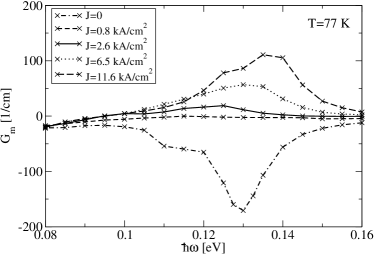
Figure 2: Gain spectrum for the quantum cascade laser of Ref. Sirtori et al., 1998 evaluated from the quantum transport model with Coulomb gauge and neglecting self-energy corrections.

Results for the superlattice are given in Fig. 3. The real part of the conductivity essentially follows the result from the simple 2-time miniband model Ktitorov et al. (1972)

$$\sigma(\omega)=\frac{J_{\mathrm{M}B}(F)}{F}\frac{1-\omega_{B}\tau_{m}\tau_{e}-{\rm i}\omega\tau_{e}}{(\omega_{B}^{2}-\omega^{2})\tau_{m}\tau_{e}+1-{\rm i}\omega(\tau_{m}+\tau_{e})}$$ (21)

with $\omega_{B}=eFd/\hbar$. Thus, this simple model gives, at least for wide minibands and high temperatures, reliable results.

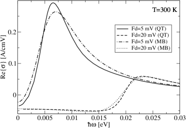
Figure 3: Real part of the dynamical conductance for the superlattice structure of Ref. Allen et al., 1991. Full and dashed line: Result from the quantum transport model with Coulomb gauge and neglecting self-energy corrections for $Fd=5$ mV and 20 mV, respectively. Dotted and dash-dotted line: Corresponding results from the 2-time miniband model Ktitorov et al. (1972).

Now we want to study the relevance of the terms $\delta\Sigma$ in Eq. (16), which have been neglected so far. Fig. 4 shows that their inclusion barely changes the result in the Coulomb gauge (the full and dashed lines are almost indistinguishable). Therefore these self-energy corrections may be neglected (at least for diagonal self-energies assumed here) allowing for a significant reduction of the numerical effort. In contrast, in the case of the Lorentz gauge, the terms evaluated with self-energy corrections (dash-dotted line) differ substantially from the simpler version without these terms (dotted line). The difference is particularly strong in the case of the superlattice, where the diagonal terms in the perturbation potential (18) are essential for the transition. Furthermore, the results of Coulomb gauge and Lorentz gauge are almost identical if the self-energy corrections are included. This demonstrates that the inclusion of these terms is essential to obtain a consistent theory, which must be independent of the choice of the gauge.

Figure 4: Comparison of different choices of the gauge and self-energy corrections $\delta\Sigma$ for (a) the superlattice at $Fd=20$ and (b) the quantum cascade laser at $Fd=260$ mV. Full line: Coulomb gauge neglecting $\delta\Sigma$; Dotted line: Lorentz gauge neglecting $\delta\Sigma$; Dashed line: Coulomb gauge with $\delta\Sigma$ (falls together with the full line); Dash-dotted line: Lorentz gauge with $\delta\Sigma$.

IV Conclusion

A formulation of the theory of nonequilibrium Green functions has been given which allows for a quantitative description of current-induced gain in semiconductor heterostructures. Quantitative agreement with the experiment for the gain spectrum of a quantum cascade laser was obtained. The standard 2-time miniband model for the superlattice could be verified for a large miniband width and under room temperature operation. The numerical results are not sensitive to the choice of the gauge if the variations of self-energy terms are taken into account. These terms are of particular importance for the Lorentz gauge, while their contribution is small in the Coulomb gauge in the calculations presented here.

Appendix A Derivation of the equations for the stationary state

The Green functions are determined by the Dyson Equation (see, e.g., chapter 5 of Ref. Haug and Jauho, 1996)

$${\rm i}\hbar\frac{\partial}{\partial t_{1}}G^{\text{ret/adv}}_{\alpha_{1},\alpha_{2}}(t_{1},t_{2})-\sum_{\beta}U_{\alpha_{1},\beta}(t_{1})G^{\text{ret/adv}}_{\beta,\alpha_{2}}(t_{1},t_{2})-\sum_{\beta}\int\frac{{\rm d}t}{\hbar}\Sigma^{\text{ret/adv}}_{\alpha_{1},\beta}(t_{1},t)G^{\text{ret/adv}}_{\beta,\alpha_{2}}(t,t_{2})\\ =\hbar\delta(t_{1}-t_{2})\delta_{\alpha_{1},\alpha_{2}}$$ (22)

and the Keldysh relation, see also Appendix B.

$$G^{<}_{\alpha_{1},\alpha_{2}}(t_{1},t_{2})=\sum_{\beta,\beta^{\prime}}\int\frac{{\rm d}t}{\hbar}\int\frac{{\rm d}t^{\prime}}{\hbar}G^{\text{ret}}_{\alpha_{1},\beta}(t_{1},t)\Sigma^{<}_{\beta,\beta^{\prime}}(t,t^{\prime})G^{\text{adv}}_{\beta^{\prime},\alpha_{2}}(t^{\prime},t_{2})\,.$$ (23)

Now we consider the stationary state, where $G(t_{1},t_{2})=\tilde{G}(t_{1}-t_{2})$. Eqs. (22,23) become:

$${\rm i}\hbar\frac{\partial}{\partial t}\tilde{G}^{\text{ret/adv}}_{\alpha_{1},\alpha_{2}}(t)-\sum_{\beta}\tilde{U}_{\alpha_{1},\beta}\tilde{G}^{\text{ret/adv}}_{\beta,\alpha_{2}}(t)-\sum_{\beta}\int\frac{{\rm d}t^{\prime}}{\hbar}\tilde{\Sigma}^{\text{ret/adv}}_{\alpha_{1},\beta}(t-t^{\prime})\tilde{G}^{\text{ret/adv}}_{\beta,\alpha_{2}}(t^{\prime})=\hbar\delta(t)\delta_{\alpha_{1},\alpha_{2}}$$ (24)

$$\tilde{G}^{<}_{\alpha_{1},\alpha_{2}}(t)=\sum_{\beta,\beta^{\prime}}\int\frac{{\rm d}t^{\prime}}{\hbar}\int\frac{{\rm d}t^{\prime\prime}}{\hbar}\tilde{G}^{\text{ret}}_{\alpha_{1},\beta}(t-t^{\prime})\tilde{\Sigma}^{<}_{\beta,\beta^{\prime}}(t^{\prime}-t^{\prime\prime})\tilde{G}^{\text{adv}}_{\beta^{\prime},\alpha_{2}}(t^{\prime\prime})\,.$$ (25)

and their Fourier-transformation (6) provides us with Eqs. (7,8).

Appendix B A remark on Eq. (5.11) of Ref. Haug and Jauho, 1996

Eq. (23) is a particular solution of the inhomogeneous differential equations (5.3) of Ref. Haug and Jauho, 1996, which are given more explicitly in Eqs. (106-107) of Ref. Wacker, 2002 in the notation used here. The Keldysh relation (5.11) derived in Ref. Haug and Jauho, 1996 contains an additional term:

$${\bf G}_{\textrm{add}}^{<}(t_{1},t_{2})=\int\frac{{\rm d}t_{b}}{\hbar}\int\frac{{\rm d}t_{c}}{\hbar}\left[\hbar\delta(t_{1}-t_{b}){\bf 1}+{\bf G}^{\mathrm{ret}}(t_{1},t_{b}){\bf U}(t_{b})+\int\frac{{\rm d}t_{a}}{\hbar}{\bf G}^{\mathrm{ret}}(t_{1},t_{a})\bm{\Sigma}^{\mathrm{ret}}(t_{a},t_{b})\right]\\ \times{\bf G}_{0}^{<}(t_{b},t_{c})\left[\hbar\delta(t_{c}-t_{2}){\bf 1}+{\bf U}(t_{c}){\bf G}^{\mathrm{adv}}(t_{c},t_{2})+\int\frac{{\rm d}t_{d}}{\hbar}\bm{\Sigma}^{\mathrm{ret}}(t_{c},t_{d}){\bf G}^{\mathrm{adv}}(t_{d},t_{2})\right]$$ (26)

This term constitutes a homogeneous solution of the inhomogeneous differential equations (for fixed $\Sigma$ and $G^{\text{ret/adv}}$) which guarantees that $G^{<}\to G^{<}_{0}$ for $t_{1},t_{2}\to-\infty$. This satisfies a general assumption underlying the perturbation expansion of the $S$-matrix. In the following we show that $G^{<}_{\textrm{add}}$ vanishes for finite times $t_{1},t_{2}$.

Using Eqs. (108,109) of Ref. Wacker, 2002 one obtains

$$\begin{split}{\bf G}_{\textrm{add}}^{<}(t_{1},t_{2})=&\int\frac{{\rm d}t_{a}}{\hbar}\int\frac{{\rm d}t_{c}}{\hbar}{\bf G}^{\mathrm{ret}}(t_{1},t_{a})\left(-{\rm i}\hbar\frac{\partial^{\mathrm{left}}}{\partial t_{a}}-{\bf E}\right){\bf G}_{0}^{<}(t_{a},t_{c})\left({\rm i}\hbar\frac{\partial}{\partial t_{c}}-{\bf E}\right){\bf G}^{\mathrm{adv}}(t_{c},t_{2})\\ =&\int\frac{{\rm d}t_{a}}{\hbar}\int\frac{{\rm d}t_{c}}{\hbar}{\bf G}^{\mathrm{ret}}(t_{1},t_{a})\left({\rm i}\hbar\frac{\partial}{\partial t_{a}}-{\bf E}\right){\bf G}_{0}^{<}(t_{a},t_{c})\left({\rm i}\hbar\frac{\partial}{\partial t_{c}}-{\bf E}\right){\bf G}^{\mathrm{adv}}(t_{c},t_{2})\\ &-{\rm i}\left[\int\frac{{\rm d}t_{c}}{\hbar}{\bf G}^{\mathrm{ret}}(t_{1},t_{a}){\bf G}_{0}^{<}(t_{a},t_{c})\left({\rm i}\hbar\frac{\partial}{\partial t_{c}}-{\bf E}\right){\bf G}^{\mathrm{adv}}(t_{c},t_{2})\right]_{t_{a}=-\infty}^{t_{a}=\infty}\,,\end{split}$$ (27)

where $\partial^{\mathrm{left}}$ means that the derivative operates to the left. In the second line, partial integration has been used. As $\left({\rm i}\hbar\frac{\partial}{\partial t_{a}}-{\bf E}\right){\bf G}_{0}^{<}(t_{a},t_{c})=0$, the first term vanishes. Furthermore, at the upper bound ${\bf G}^{\mathrm{ret}}(t_{1},\infty)=0$ holds for finite times $t_{1}$. Applying the same manipulations for $t_{c}$, we find

$$\begin{split}{\bf G}_{\textrm{add}}^{<}(t_{1},t_{2})=&{\rm i}\int\frac{{\rm d}t_{c}}{\hbar}{\bf G}^{\textrm{ret}}(t_{1},-\infty){\bf G}_{0}^{<}(-\infty,t_{c})\left({\rm i}\hbar\frac{\partial}{\partial t_{c}}-{\bf E}\right){\bf G}^{\textrm{adv}}(t_{c},t_{2})\\ =&{\bf G}^{\textrm{ret}}(t_{1},-\infty){\bf G}_{0}^{<}(-\infty,-\infty){\bf G}^{\textrm{adv}}(-\infty,t_{2})\,.\end{split}$$ (28)

For a real system the retarded and advanced Green functions decay for large time differences and we find ${\bf G}_{\textrm{add}}^{<}(t_{1},t_{2})\to 0$ for finite $t_{1},t_{2}$. Therefore this additional term is spurious.

A second, more physical argument relates to the idea, that the stationary state of a real physical system should not depend on the initial conditions used in a formal theory. Except for specific situations exhibiting a hysteresis, scattering processes will install a stationary state which is independent of initial conditions. Therefore all additional homogeneous solutions should reflect transient effects, which vanish if the initial state is chosen at $t_{1}=-\infty$ and $t_{2}=-\infty$.

Appendix C Derivation of Eqs. (15,16)

Setting $U(t)=\tilde{U}+\delta U(t)$, $G(t_{1},t_{2})=\tilde{G}(t_{1}-t_{2})+\delta G(t_{1},t_{2})$ and $\Sigma(t_{1},t_{2})=\tilde{\Sigma}(t_{1}-t_{2})+\delta\Sigma(t_{1},t_{2})$ in Eqs. (22,23) gives in linear order $\delta U$:

$${\rm i}\hbar\frac{\partial}{\partial t_{1}}\delta G^{\text{ret}}_{\alpha_{1},\alpha_{2}}(t_{1},t_{2})-\sum_{\beta}\tilde{U}_{\alpha_{1},\beta}\delta G^{\text{ret}}_{\beta,\alpha_{2}}(t_{1},t_{2})-\sum_{\beta}\int\frac{{\rm d}t}{\hbar}\tilde{\Sigma}^{\text{ret}}_{\alpha_{1},\beta}(t_{1}-t)\delta G^{\text{ret}}_{\beta,\alpha_{2}}(t,t_{2})=\\ \sum_{\beta}\delta U_{\alpha_{1},\beta}(t_{1})\tilde{G}^{\text{ret}}_{\beta,\alpha_{2}}(t_{1}-t_{2})+\sum_{\beta}\int\frac{{\rm d}t}{\hbar}\delta\Sigma^{\text{ret}}_{\alpha_{1},\beta}(t_{1},t)\tilde{G}^{\text{ret}}_{\beta,\alpha_{2}}(t-t_{2})$$ (29)

This constitutes an inhomogeneous differential equation, where the homogeneous part (left-hand side) is identical with the defining equation (24) for $\tilde{G}^{\text{ret}}$. Thus $\tilde{G}^{\text{ret}}$ is the corresponding Green function and the solution is given by:

$$\delta{\bf G}^{\text{ret}}(t_{1},t_{2})=\int\frac{{\rm d}t}{\hbar}\int\frac{{\rm d}t^{\prime}}{\hbar}\tilde{\bf G}^{\text{ret}}(t_{1}-t)\Big{[}\delta{\bf U}(t)\hbar\delta(t-t^{\prime})+\delta\bm{\Sigma}^{\text{ret}}(t,t^{\prime})\Big{]}\tilde{\bf G}^{\text{ret}}(t^{\prime}-t_{2})$$ (30)

and Fourier transformation using Eq. (14) gives Eq. (15) after some algebra. $\delta G^{\text{adv}}$ is evaluated in the same way with ret replaced by adv.

The linearization of the Keldysh relation (23) provides us with

$$\delta{\bf G}^{<}(t_{1},t_{2})=\int\frac{{\rm d}t}{\hbar}\int\frac{{\rm d}t^{\prime}}{\hbar}\Big{[}\delta{\bf G}^{\text{ret}}(t_{1},t)\tilde{\bm{\Sigma}}^{<}(t-t^{\prime})\tilde{\bf G}^{\text{adv}}(t^{\prime}-t_{2})+\tilde{\bf G}^{\text{ret}}(t_{1}-t)\delta\bm{\Sigma}^{<}(t,t^{\prime})\tilde{\bf G}^{\text{adv}}(t^{\prime}-t_{2})\\ +\tilde{\bf G}^{\text{ret}}(t_{1}-t)\tilde{\bm{\Sigma}}^{<}(t-t^{\prime})\delta{\bf G}^{\text{adv}}(t^{\prime},t_{2})\Big{]}$$ (31)

Fourier transformation gives Eq. (16) after some algebra.

Appendix D Choice of gauges

We study the linear response to an external radiation field propagating in $y$-direction

$$\vec{F}(\vec{r},t)=\int\frac{{\rm d}\omega}{2\pi}F(\omega)\vec{e}_{z}{\rm e}^{{\rm i}k(\omega)y-{\rm i}\omega t}\qquad\vec{B}(\vec{r},t)=\int\frac{{\rm d}\omega}{2\pi}\frac{k(\omega)}{\omega}F(\omega)\vec{e}_{x}{\rm e}^{{\rm i}k(\omega)y-{\rm i}\omega t}\,.$$ (32)

Thus we have two reasonable choices of the electromagnetic potentials Jackson (1998):

Coulomb gauge $$\quad\vec{A}(\vec{r},t) =\int\frac{{\rm d}\omega}{2\pi}\frac{F(\omega)}{{\rm i}\omega}\vec{e}_{z}{\rm e}^{{\rm i}k(\omega)y-{\rm i}\omega t} \quad\phi(\vec{r},t) =0$$ (33)

Lorentz gauge $$\quad\vec{A}(\vec{r},t) =-\int\frac{{\rm d}\omega}{2\pi}\frac{k(\omega)F(\omega)z}{\omega}\vec{e}_{y}{\rm e}^{{\rm i}k(\omega)y-{\rm i}\omega t} \quad\phi(\vec{r},t) =-F(\omega)z{\rm e}^{{\rm i}k(\omega)y-{\rm i}\omega t}$$ (34)

In the spirit of a dipole approximation (i.e., assuming that the wavelength is large compared to the size of the active region) the terms containing $k$ are neglected, providing the expressions (17,18) in the perturbation Hamiltonian, where quadratic terms $\propto F(\omega)^{2}$ are neglected.

References

• Esaki and Tsu (1970) L. Esaki and R. Tsu, IBM J. Res. Develop. 14, 61 (1970).
• Kazarinov and Suris (1971) R. F. Kazarinov and R. A. Suris, Sov. Phys. Semicond. 5, 707 (1971).
• Faist et al. (1994) J. Faist, F. Capasso, D. L. Sivco, C. Sirtori, A. L. Hutchinson, and A. Y. Cho, Science 264, 553 (1994).
• Köhler et al. (2002) R. Köhler, A. Tredicucci, F. Beltram, H. E. Beere, E. H. Linfield, A. G. Davies, D. A. Ritchie, R. C. Iotti, and F. Rossi, Nature 417, 156 (2002).
• Gmachl et al. (2001) C. Gmachl, F. Capasso, D. L. Sivco, and A. Y. Cho, Rep. Prog. Phys. 64, 1533 (2001).
• Ktitorov et al. (1972) S. A. Ktitorov, G. S. Simin, and V. Y. Sindalovskii, Sov. Phys.–Sol. State 13, 1872 (1972), [Fizika Tverdogo Tela 13, 2230 (1971)].
• Renk et al. (1998) K. F. Renk, E. Schomburg, A. A. Ignatov, J. Grenzer, S. Winnerl, and K. Hofbeck, Physica B 244, 196 (1998).
• Wacker et al. (1997) A. Wacker, S. J. Allen, J. S. Scott, M. C. Wanke, and A.-P. Jauho, phys. status solidi (b) 204, 95 (1997).
• Kroemer (2000) H. Kroemer, Large-amplitude oscillation dynamics and domain suppression in a superlattice Bloch oscillator (2000), arXiv: cond-mat/0009311.
• Allen et al. (1991) S. J. Allen, J. S. Scott, M. C. Wanke, K. Maranowsky, A. C. Gossard, M. J. W. Rodwell, and D. H. Chow, in Terahertz Sources and Systems, edited by R. E. Miles, P. Harrison, and D. Lippens (Kluwer Academic Publishers, Dordrecht, 1991).
• Wacker (2002) A. Wacker, Phys. Rep. 357, 1 (2002).
• Jackson (1998) J. D. Jackson, Classical Electrodynamics (John Wiley & Sons, New York, 1998), 3rd ed.
• Tucker and Feldman (1985) J. R. Tucker and M. J. Feldman, Rev. Mod. Phys. 57, 1055 (1985).
• Platero and Aguado (1997) G. Platero and R. Aguado, Appl. Phys. Lett. 70, 3546 (1997).
• Haug and Koch (1994) H. Haug and S. Koch, Quantum theory of the optical and electronic properties of semiconductors (World Scientific, Singapore, 1994).
• Kadanoff and Baym (1962) L. P. Kadanoff and G. Baym, Quantum Statistical Mechanics (Benjamin, New York, 1962).
• Schmitt-Rink et al. (1988) S. Schmitt-Rink, D. S. Chemla, and H. Haug, Phys. Rev. B 37, 941 (1988).
• Haug and Jauho (1996) H. Haug and A.-P. Jauho, Quantum Kinetics in Transport and Optics of Semiconductors (Springer, Berlin, 1996).
• Henneberger and Koch (1996) K. Henneberger and S. W. Koch, Phys. Rev. Lett. 76, 1820 (1996).
• Pereira, Jr. and Henneberger (1998) M. F. Pereira, Jr. and K. Henneberger, Phys. Rev. B 58, 2064 (1998).
• Lipavský et al. (1986) P. Lipavský, V. Špička, and B. Velický, Phys. Rev. B 34, 6933 (1986).
• Datta (1995) S. Datta, Electronic Transport in Mesoscopic Systems (Cambridge University Press, Cambridge, 1995).
• Lake et al. (1997) R. Lake, G. Klimeck, R. C. Bowen, and D. Jovanovic, J. Appl. Phys. 81, 7845 (1997).
• Wacker and Hu (1999) A. Wacker and B. Y.-K. Hu, Phys. Rev. B 60, 16039 (1999).
• Sirtori et al. (1998) C. Sirtori, P. Kruck, S. Barbieri, P. Collot, J. Nagle, M. Beck, J. Faist, and U. Oesterle, Appl. Phys. Lett. 73, 3486 (1998).
• Wacker et al. (1999) A. Wacker, A.-P. Jauho, S. Rott, A. Markus, P. Binder, and G. H. Döhler, Phys. Rev. Lett. 83, 836 (1999).
• Lee and Wacker (2002) S.-C. Lee and A. Wacker, Physica E 13, 858 (2002).
• Bonilla (1995) L. L. Bonilla, in Nonlinear Dynamics and Pattern Formation in Semiconductors and Devices, edited by F.-J. Niedernostheide (Springer, Berlin, 1995), chap. 1, pp. 1–20.
• Patra et al. (1998) M. Patra, G. Schwarz, and E. Schöll, Phys. Rev. B 57, 1824 (1998).
• Iotti and Rossi (2001) R. C. Iotti and F. Rossi, Phys. Rev. Lett. 87, 146603 (2001).
• Shik (1975) A. Y. Shik, Sov. Phys. Semicond. 8, 1195 (1975), [Fiz. Tekh. Poluprov. 8, 1841 (1974)].
• Wacker and Jauho (1998) A. Wacker and A.-P. Jauho, Phys. Rev. Lett. 80, 369 (1998).
• Eickemeyer et al. (2000) F. Eickemeyer, R. A. Kaindl, M. Woerner, T. Elsaesser, S. Barbieri, P. Kruck, C. Sirtori, and J. Nagle, Appl. Phys. Lett. 76, 3254 (2000).