Internal localized eigenmodes on spin discrete breathers in antiferromagnetic chains with on-site easy axis anisotropy

Abstract

We investigate internal localized eigenmodes of the linearized equation around spin discrete breathers in 1D antiferromagnets with on-site easy axis anisotropy. The threshold of occurrence of the internal localized eigenmodes has a typical structure in parameter space depending on the frequency of the spin discrete breather. We also performed molecular dynamics simulation in order to show the validity of our linear analysis.

Discrete breathers (DB’s) are the time-periodic and spatially localized excitations on the nonlinear lattice with translational invariance [1, 2], which are also called intrinsic localized modes in the literatures [3]. The existence of DB’s was mathematically proved in the anticontinuous limit [4]. Both the discreteness and the nonlinearity play a crucial role in the existence of DB’s. The spatial discreteness is quite common in nature, particularly in condensed matter physics. Recently the experimental realization of a DB was performed in anisotropic antiferromagnets [5] and Josephson junction ladders [6].

In magnetic systems, both the spin-spin exchange interaction and the on-site spin anisotropy are intrinsically nonlinear, so that it is quite natural to predict the existence of DB’s. Since the dissipation of spin waves in magnetic materials is usually weak compared with that of lattice vibrations in crystals, the spin lattice model has obvious advantages over lattice vibration models from the experimental point of views. Lai and Sievers have extensively studied the DB’s of spin wave, namely spin DB’s, for various situations of antiferromagnets [7]. The spin DB’s have also been recently studied in ferromagnetic lattices [8].

The DB can play a role of the scattering center affecting energy transport by scattering, absorbing or radiating phonons. The scattering properties of the DB are closely related to the structure of the eigenmodes of the linearized equation around the DB itself [9, 10, 11, 12], which will be called internal localized eigenmodes (ILE’s). In particular, it was shown that the perfect transmission occurs at the ILE threshold, which should be tangent to the phonon band edge with the zero wave number [10, 11]. However, when the ILE’s on DB’s penetrate the phonon band, the well known Fano resonances are obtained [12]. These results can be directly applied to the spin lattice model considering the analogy between the lattice vibration (phonon) and the rotation of spin (magnon or spin wave).

In this paper, we present the existence of the ILE’s on spin DB’s using the linearized equation of spin DB’s in one-dimensional (1D) antiferromagnets with on-site easy axis anisotropy. The thresholds of the ILE’s show some special structure in parameter space. The comparison between the prediction from linear analyses and the results of molecular dynamics (MD) simulation will also be presented.

Let us consider the antiferromagnetic chain of N spins with the Hamiltonian [13]

$$H=2J\sum_{n}{\bf S}_{n}\cdot{\bf S}_{n+1}-D\sum_{n}(S_{n}^{z})^{2},$$ (1)

where the positive $J$ and $D$ are the exchange constant and the single ion anisotropy constant, respectively. Hence, the antiferromagnetic ordering and aligning with $z$ direction of each spin are energetically more favorable in the ground state.

Using the well known Heisenberg equation of motion

$$i\hbar\frac{d{\bf S}_{n}}{dt}=[{\bf S}_{n},H]$$ (2)

with $s_{n}^{\pm}=(S_{n}^{x}\pm iS_{n}^{y})/S$, the nonlinear equation of motion for $s_{n}^{+}$ can be obtained in the following

$$i\hbar\frac{ds_{n}^{+}}{dt} = -2JS[(s_{n-1}^{z}+s_{n+1}^{z})s_{n}^{+}-(s_{n-1}^{+}+s_{n+1}^{+})s_{n}^{z}]$$ (3)

$$+ 2DSs_{n}^{z}s_{n}^{+}.$$ (4)

If we assume a solution of the form $s_{n}^{+}=s_{n}e^{-i\omega t}$, the stationary spin DB can be obtained by using the following equation

$$\tilde{\hbar}\omega s_{n} = (-1)^{n}\{C(\sqrt{1-s_{n-1}^{2}}+\sqrt{1-s_{n+1}^{2}})s_{n}$$ (5)

$$+ [C(s_{n-1}+s_{n+1})+s_{n}]\sqrt{1-s_{n}^{2}}\},$$ (6)

where $\tilde{\hbar}=\hbar/2DS$ and $C=J/D$. In this paper we consider only a single non-moving spin DB. The familiar dispersion relation of the extended spin wave modes, $\tilde{\hbar}\omega=\pm\sqrt{(1+2C)^{2}-4C^{2}\cos^{2}ka}$, can also be obtained by Eq. (5) by putting

$$\left(\begin{array}[]{c}s_{2n}\\ s_{2n+1}\end{array}\right)=\left(\begin{array}[]{c}f_{0}e^{2ikna}\\ f_{1}e^{ik(2n+1)a}\end{array}\right),$$ (7)

where $a$ is the lattice spacing, and $|f_{0}|$, $|f_{1}|\ll 1$. The linearized equation of Eq. (3) near the spin DB for $\xi_{n}(t)=s_{n}^{+}(t)-s_{n}e^{-i\omega_{b}t}$ is given by

$$i\tilde{\hbar}\dot{\xi_{n}} = (-1)^{n}\{C[(A_{n-1}+A_{n+1})\xi_{n}-s_{n}(B_{n-1}Re(\xi_{n-1})$$ (8)

$$+ B_{n+1}Re(\xi_{n+1}))+A_{n}(\xi_{n-1}+\xi_{n+1})-B_{n}(s_{n-1}$$ (9)

$$+ s_{n+1})Re(\xi_{n})]+A_{n}\xi_{n}-s_{n}B_{n}Re(\xi_{n})\}-\tilde{\hbar}\omega_{b}\xi_{n},$$ (10)

where $A_{n}=\sqrt{1-s_{n}^{2}}$, $B_{n}=s_{n}/2\sqrt{1-s_{n}^{2}}$, and $Re(\xi)$ is the real part of $\xi$. The above Floquet (or linear) equation is written in the form $d\vec{\xi}/dt=M\vec{\xi}$. By diagonalizing the matrix $M$, the eigenmodes for small perturbation of spin DB’s are obtained. Let us note that there exist two important system parameters, the relative strength of the exchange interaction, $C(=J/D)$ and the frequency of spin DB, $\omega_{b}$.

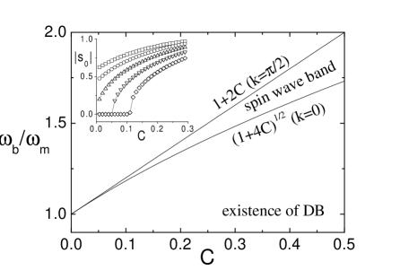
FIG. 1.: The band structure of spin waves as a function of $C$. The inset represents the amplitude of the spin oscillation at the central site of spin DB as a function of $C$ for a given frequency of spin DB $\omega_{b}$. From the upper they correspond to $\omega_{b}/\omega_{m}=$ 0.8, 0.9 1.0, 1.1 and 1.2, respectively.

Without the exchange interaction, i.e. $J=0$, the resonance frequency of a local nonlinear oscillator is limited to $\omega_{m}=1/\tilde{\hbar}$ since the nonlinearity of the individual system is soft. In the case $\omega_{b}/\omega_{m}>1$, spin DB’s cannot exist in the small coupling limit ($J\rightarrow 0$), so that we obtain two distinct regions for $\omega_{b}$ such as $\omega_{b}/\omega_{m}>1$ and $\omega_{b}/\omega_{m}<1$. In the former case ($\omega_{b}/\omega_{m}>1$) the spin DB’s can exist only above the certain critical value of $C$, which can be explained by considering a new on-site potential modified by the neighboring sites. For simplicity let’s consider just three spins, namely, ones on the sites $-1$, $0$, and $1$, where the site $0$ corresponds to the center of the spin DB. In the weak coupling limit the dynamics of the neighboring spins at the sites $\pm 1$ can be described by simple harmonic oscillation with a small amplitude $\epsilon$, assuming the spin DB solution. From Eq. (5) we can obtain the following equation for the frequency of the spin precession at the site $0$

$$\tilde{\hbar}\omega s_{0}=2Cs_{0}\sqrt{1-\epsilon^{2}}+(2C\epsilon+s_{0})\sqrt{1-s_{0}^{2}}.$$ (11)

Considering $\epsilon<<s_{0}\leq 1$ in the weak coupling limit, the above equation can be approximated to $\omega/\omega_{m}\approx 2C+\sqrt{1-s_{0}^{2}}$, so that the new maximum frequency of local nonlinear oscillators, namely $\omega_{m}^{\prime}$, is given by $\omega_{m}(2C+1)$, which means that the possible maximum frequency of a spin DB also increases under the coupling with the neighboring spins. Actually this relation exactly coincides with the $k=\pi/2$ band edge of the spin wave as shown in Fig. 1 in the weak coupling limit. Taking into account the instability caused by the resonance between DB’s and phonons [1], we should exclude the overlapping region between spin DB and the spin wave band, so that finally the border of the existence of spin DB’s is given by the $k=0$ band edge, $\omega_{m}^{\prime}/\omega_{m}=\sqrt{1+4C}$. The inset of Fig. 1 shows the amplitude of the spin oscillation at the central site of spin DB as a function of $C$ for a given frequency of spin DB $\omega_{b}$, where the criteria mentioned above can be also confirmed numerically. In other words, the frequencies of spin DB’s are always located below the spin wave band, which is nothing new in the sense of general criteria for the existence of a DB. We would like to mention, however, that this leads to somewhat interesting consequences that a spin DB appears above some critical coupling strength, and disappears in the anticontinuous limit with the frequency of a spin DB fixed. The mathematical proof for the existence of DB’s was performed in this limit [4].

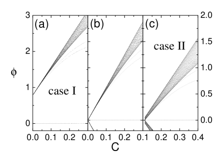
FIG. 2.: Floquet spectrum for (a) $\omega_{b}/\omega_{m}=0.8$ (b) $\omega_{b}/\omega_{m}=1.0$, and (c) $\omega_{b}/\omega_{m}=1.2$. See the left tick labels for (a) and the right tick labels for both (b) and (c).

Figure 2 shows the evolution of the eigenvalues of the Floquet matrix $M$ on unit circle (the angle $\phi$ of the eigenvalue $e^{i\phi}$) as a function of $C$ for several $\omega_{b}$’s, where both spin wave bands and the detached branches are clearly seen. For all calculations we take $\tilde{\hbar}=1$. The eigenmodes coming from the bottom of the band are observed to be the ones which are localized. These are ILE’s mentioned above. The ILE’s belong to either symmetric or antisymmetric eigenmodes with respect to their reflection symmetry to the center of a spin DB. While for $\omega_{b}/\omega_{m}<1$ two ILE’s appear simultaneously at $C=0$ [Fig.2(a)], for $\omega_{b}/\omega_{m}>1$ at first the symmetric ILE appears at a certain value of $C$ and then the antisymmetric one appears at larger $C$ [Fig. 2(c)]. We call the former the case I and the latter the case II.

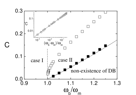
FIG. 3.: The threshold of occurrences of symmetric (the filled squares) and antisymmetric (the open squares) ILE’s as a function of the frequency of the spin DB. Spin DB’s cannot exist in the region under the solid line (see the text for details). In the inset we replot the threshold of the antisymmetric ILE’s (the open squares) in log-log scale, which clearly shows power law dependence.

Figure 3 shows the threshold of the ILE’s as a function of $\omega_{b}$, where the dashed vertical line $\omega_{b}/\omega_{m}=1$, at which two spin wave bands collide each other as shown in Fig. 2(b), divides the parameter space into two regions for the thresholds of ILE’s (i.e. the case I and II). The solid line represents the border of the existence of spin DB’s described by $C=[(\omega_{b}/\omega_{m})^{2}-1]/4$, below which the spin DB’s cannot exist. It is mentioned that the threshold of the symmetric ILE (the filled squares) looks like the straight line, and that of the antisymmetric one (the open squares) shows the power law dependence, namely $C\propto\omega_{b}^{0.72}$ as shown in the inset of Fig. 3. This threshold behavior was also observed in the case of Klein-Gordon (KG) chain with $\phi^{4}$ (double well) on-site potential described by $V(x)=(x^{4}-2x^{2})/4$ [14], where $\omega_{b}=2/3$, at which two neighboring phonon band edges with $k=0$ collide each other, play a similar role as $\omega_{b}/\omega_{m}=1$ in our antiferromagnet. However, this frequency does not correspond to the maximum frequency of the local soft nonlinear oscillator, which is $\omega_{m}=1$ in a $\phi^{4}$ KG chain. It should also be noted that in other KG chains with Morse ($V(x)=[1-\exp(-x)]^{2}/2$) or cubic [$V(x)=x^{2}/2-x^{3}/3$] on-site potential this is not the case, where for all $\omega_{b}(<\omega_{m}=1)$ the cubic and the Morse potential correspond only to the case I and the case II, respectively. This has not been understood yet.

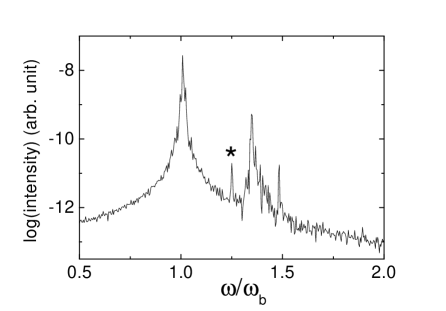
FIG. 4.: The power spectrum of $M^{y}(t)$ with $\omega_{b}/\omega_{m}=1.1$ and $C=0.3$. This is calculated using MD simulation with 103 spins during 256$T_{b}$ ($T_{b}=2\pi/\omega_{b}$) under the random noise with the intensity $D=10^{-5}$ [14]. “$\star$” indicates the symmetric ILE, above which the spin wave excitations are shown.

One of the reasons why we choose this magnetic lattice for our investigation is that experimentally the generation of a spin DB was reported in the quasi-1D biaxial antiferromagnet (C₂H₅NH₃)₂CuCl₄ [5] like the system studied in this paper. By microwave absorption experiment the peak corresponding to the spin DB was observed in the spin wave gap. The absorption spectrum measured in the experiment is proportional to the imaginary part of the dynamic magnetic susceptibility, which can be calculated using the Kubo expression [5].

$$A(\omega)\propto\int_{0}^{\infty}dt\left<M^{y}(t+t^{\prime})M^{y}(t^{\prime})\right>_{t^{\prime}}e^{i\omega t},$$ (12)

where $M^{y}(t)=\sum_{n}s_{n}^{y}(t)$ and $\left<A\right>_{t^{\prime}}$ is the time average of the variable $A$. We calculate $M^{y}(t)$ using MD simulations with 103 spins starting from the solution of a spin DB obtained from Eq. (5) under the random amplitude noise [15]. Figure 4 clearly shows that an absorption peak, which is a several order of magnitude smaller than the spin DB peak, exists between the spin DB and the spin wave band. Without noise we can obtain only the spin DB peak. Although the absorption power of this ILE is so tiny compared with that of the spin DB, it should not be ignored in comparison with that of the spin wave band. It is worth noting that only the symmetric ILE can be observed in the absorption spectrum since the antisymmetric ILE disappears when the summation, $\sum_{n}s_{n}^{y}(t)$, is performed. Figure 5 shows that the frequency of the symmetric ILE calculated using MD simulation is well fitted by the prediction of the linear theory in the region of small $C$. It is remarked that in the experiment of Ref.[5], somewhat broad spectrum of a spin DB was observed since many spin DB’s with different frequencies were excited simultaneously. In order to observe the ILE’s studied in this paper, more improved experimental status will be needed, for example, a single spin DB excitation, the suppression of volume and surface modes, better resolution in the absorption power, and so on. We also note that in general the antiferromagnetic ordering can persist only above some critical value of $C$, roughly speaking the order of one. Even though it does not seem to be easy to find out the transition from the case I to the case II in this system in experiment due to this reason, it is still possible to observe the ILE’s themselves for higher values of $C$.

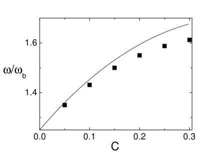
FIG. 5.: The frequency of the symmetric ILE given by the Floquet spectrum in Fig. 2 (the solid curve) and by the power spectrum of $M^{y}(t)$ using MD simulation (the filled square).

In our previous work on discrete nonlinear Schrödinger (DNLS) equation [10] we already noted that the DNLS equation is the nontrivial simplest system for studying scattering problems or ILE’s. However, it has only a single parameter since the change of the breather frequency $\omega_{b}$ can be compensated by scaling $\Omega\rightarrow\Omega/\omega_{b}$ and $C\rightarrow C/\omega_{b}$, where $\Omega$ and $C$ are the frequency of the small perturbation and the linear coupling strength, respectively. We would like to point out that the 1D antiferromagnet with easy axis anisotropy provides a good intermediate example with two spin wave bands (or scattering channels) and two parameters ($C$ and $\omega_{b}$) between the case of DNLS equation with two phonon bands and one parameter ($C/\omega_{b}$) and that of the KG chain with an infinite number of phonon bands and two parameters.

In summary we have investigated the characteristics and the possibility of experimental observation of the ILE’s in 1D antiferromagnets with easy axis anisotropy using both linear analyses and MD simulations. The structure of the thresholds of the ILE’s strongly depends on the frequency of a spin DB. For $\omega_{b}/\omega_{m}<1$ the ILE’s appear at $C=0$ simultaneously, while for $\omega_{b}/\omega_{m}>1$ the symmetric ILE occurs at first at the certain value of $C$ and then the antisymmetric one appears at the larger $C$. It is shown that the frequency of the ILE’s calculated using MD simulation is well fitted by the prediction of the linear theory. We hope that these ILE’s will be observed in experiments.

We would like to thank Sergej Flach for a careful reading of this manuscript and helpful comments. SW also thanks Mikhail Fistul for helpful discussions.

REFERENCES

- [1] S. Flach and C. R. Willis, Phys. Rep. 295, 181 (1998).
- [2] S. Aubry, Physica D 103, 201 (1997).
- [3] A. J. Sievers and S. Takeno, Phys. Rev. Lett. 61, 970 (1988).
- [4] R. S. Mackay, S. Aubry, Nonlinearity 7, 16233 (1991).
- [5] U. T. Schwarz, L. Q. English, and A. J. Sievers, Phys. Rev. Lett. 83, 223 (1999).
- [6] P. Binder, D. Abraimov, A. V. Ustinov, S. Flach, and Y. Zolotaryuk, Phys. Rev. Lett. 84, 745 (2000).
- [7] R. Lai and A. J. Sievers, Phys. Rep. 314, 147 (1999).
- [8] Y. Zolotaryuk, S. Flach, and V. Fleurov, Phys. Rev. B 63, 214422 (2001).
- [9] S. Kim, C. Baesens, and R. S. Mackay, Phys. Rev. E 56, R4955 (1997).
- [10] S. W. Kim and S. Kim, Physica D 141, 91 (2000).
- [11] S. Lee and S. Kim, Int. J. Mod. Phys. B 14, 1903 (2000).
- [12] S. W. Kim and S. Kim, Phys. Rev. B 63, 212301 (2001).
- [13] R. Lai, S. A. Kiselev, and A. J. Sievers, Phys. Rev. B 54 R12665 (1996).
- [14] S. Kim and R. S. Mackay, unpublished.
- [15] At each time step of numerical integrations of Eq. (3) we add random amplitude noises to the variables , where the absolute values of are normalized to one and represents the strength of noise. () is used as the time interval for numerical integration.