From Cooper pairs to Luttinger liquids with bosonic atoms in optical lattices

Abstract

We propose a scheme to observe typical strongly correlated fermionic phenomena with bosonic atoms in optical lattices. For different values of the sign and strength of the scattering lengths it is possible to reach a ”superconducting” regime, where the system exhibits atomic pairing, or a Luttinger liquid behavior. We identify the range of parameters where these phenomena appear, illustrate our predictions with numerical calculations, and show how to detect the presence of pairing.

After the achievement of Bose–Einstein condensation with dilute atomic gases bec , a great deal of interest in atomic physics has turned to the theoretical and experimental study of cold fermionic atoms. In particular, one of the most challanging goals nowadays is the observation of the BCS transition bcs1 , where fermionic atoms are expected to form Cooper pairs when they experience an attractive interaction. Although Fermi degeneracy has already been observed in several labs fer , the temperatures at which Cooper pairs are formed have not been reached (see, however, bcs2 ).

In this letter we propose to use bosonic atoms trapped in optical lattices to observe typical fermionic correlation phenomena, such the formation of Cooper pairs or the characteristic spin–density separation corresponding to a Luttinger liquid. Our scheme is based on the fact that strongly interacting bosons in a lattice can behave as weak (or even strong) interacting fermions. Our proposal is motivated by the recent experiment with bosons in optical lattices Bloch , where the strong interaction regime has been achieved, as it was theoretically predicted Jaksch . In fact, this experiment illustrates that our proposal can be implemented with existing technology.

The fact that strongly interacting bosons can behave as fermions is, of course, not a new idea. It is well known that the problem of one dimensional hard core bosons is exactly mapped into the one of free fermions Girardeau , since the infinite on site repulsion plays the role of an effective Pauli principle for bosons. This is the case, for instance, for the Mott phase of bosonic atoms in an optical lattice Bloch ; Jaksch , or for the Laughlin atomic liquids in rapidly rotating traps belen . In an attempt to go beyond the usual free-fermionic behavior of hard core bosons, we show that the ability of tuning the sign and strength of atomic interactions can easily make bosons behave as interacting fermions. To be more specific, we will consider bosonic atoms confined in an optical lattice in such a way that tunneling can only occur in one spatial dimension. We will assume that some internal levels have been shifted up in energy using off resonant microwave fields, so that only two internal levels can be occupied. We will concentrate in the situation in which the interaction between atoms in the same internal level, $U$, is repulsive and stronger than the interaction between atoms in different ones, $V$ footnotea . The basic mechanism behind our scheme is simple. At sufficient low temperatures and tunneling amplitude, the strong repulsion $U$ prevents two atoms with the same internal state to be in the same lattice site, so that atoms behave as interacting fermions. We will show that the interaction between the effective fermions is just the bare interaction $V$, and depending on its sign and strength a rich spectrum of possibilities can be observed.

We consider a gas of $N$ bosonic atoms in a one-dimensional optical lattice with $M$ wells, and will call $\nu=N/2M$ the filling factor. We will denote by $\sigma={\uparrow,\downarrow}$ the two relevant internal levels. The Hamiltonian describing this situation is Jaksch :

$$H=-t\sum_{<i,j>\sigma}a^{\dagger}_{i\sigma}a_{j\sigma}+U\sum_{i,\sigma}n_{i\sigma}^{2}+V\sum_{i}n_{i\uparrow}n_{i\downarrow}.$$ (1)

Here $a^{\dagger}_{i\sigma}$ and $a_{i\sigma}$ are bosonic operators that create (annihilate) an atom on the $i$–th lattice site with spin state $\sigma$, and $n_{i\sigma}=a^{\dagger}_{i\sigma}a_{i\sigma}$. The tunneling amplitude, $t$, as well as $U$ and $V$ can be easily written in terms of the scattering lengths and lattice parameters Jaksch .

Let us analyze first the simple limiting case $U\to\infty$, where the atoms with the same spin are not allowed to be at the same lattice site. The ground state and low-energy excitations of Hamiltonian (1) lie within the subspace generated by states of the form:

$$|\mathbf{x},\mathbf{y}\rangle=a^{\dagger}_{x_{1}\uparrow}\ldots a^{\dagger}_{x_{N_{\uparrow}}\uparrow}\,a^{\dagger}_{y_{1}\downarrow}\ldots a^{\dagger}_{y_{N_{\downarrow}}\downarrow}|0\rangle,$$ (2)

where $N_{\uparrow}+N_{\downarrow}=N$, $\mathbf{x}=(x_{1},\ldots,x_{N_{\uparrow}})$, and $\mathbf{y}=(y_{1},\ldots,y_{N_{\downarrow}})$ denote, respectively, the sites occupied by the particles with spin up and spin down, and $x_{i}\neq x_{j}$, $y_{i}\neq y_{j}$, $\forall i\neq j$. This projected bosonic Hilbert space is isomorphic to the Hilbert space of fermions with spin $1/2$ in a one-dimensional lattice. The bosonic operators can be transformed into fermionic ones by the well known Jordan-Wigner transformation Jordan :

$$a^{\dagger}_{i\sigma}=(-1)^{\sum_{j<i}(1-2c^{\dagger}_{j\sigma}c_{j\sigma})}c^{\dagger}_{i\sigma},$$ (3)

where the operator $c^{\dagger}_{j\sigma}$ creates an effective fermion in the $j$–th site with spin $\sigma$. With the transformation (3) the bosonic Hamiltonian (1) projected to the subspace (2) is exactly transformed footnotec into a Hubbard chain of fermions:

$$H_{F}=-t\sum_{<i,j>\sigma}c^{\dagger}_{i\sigma}c_{j\sigma}+V\sum_{i}c^{\dagger}_{i\uparrow}c_{i\uparrow}c^{\dagger}_{i\downarrow}c_{i\downarrow},$$ (4)

where the parameters $t$ and $V$ coincide with those appearing in Hamiltonian (1).

Given the fact that the projected Hamiltonian and (4) are the same, they have exactly the same spectrum. The bosonic eigenstates are related to the fermionic eigenstates by the following correspondence: $|\Psi_{F}\rangle=\sum_{\mathbf{x},\mathbf{y}}f_{F}(\mathbf{x},\mathbf{y})\,\,|\mathbf{x},\mathbf{y}\rangle_{F}$ $\rightarrow$ $\sum_{\mathbf{x},\mathbf{y}}f_{B}(\mathbf{x},\mathbf{y})\,\,|\mathbf{x},\mathbf{y}\rangle=|\Psi_{B}\rangle$. Here, $|\mathbf{x},\mathbf{y}\rangle_{F}=c^{\dagger}_{x_{1}\uparrow}\ldots c^{\dagger}_{x_{N_{\uparrow}}\uparrow}c^{\dagger}_{y_{1}\downarrow}\ldots c^{\dagger}_{y_{N_{\downarrow}}\downarrow}|0\rangle$, $|\mathbf{x},\mathbf{y}\rangle$ is given by (2), and $f_{F}(\mathbf{x},\mathbf{y})$, $f_{B}(\mathbf{x},\mathbf{y})$, the fermionic and bosonic amplitudes for the configuration $(\mathbf{x},\mathbf{y})$, are related by a sign factor in the form $f_{B}(\mathbf{x},\mathbf{y})=\mathrm{sgn}(\mathbf{x},\mathbf{y})f_{F}(\mathbf{x},\mathbf{y})=\prod_{i<j}\mathrm{sgn}(x_{i}-x_{j})\mathrm{sgn}(y_{i}-y_{j})\,f_{F}(\mathbf{x},\mathbf{y})$.

The physics of the fermionic Hubbard chain has been extensively studied (see, e.g., hub1 ). Depending on the sign of $V$ and on the ratio $V/t$ the system is known to exhibit different phenomena. In order to determine which of these phenomena can be observed with a real bosonic system we have to address two questions. First, since $U$ cannot be infinite, we have to determine the conditions on $U$ such that the above treatment remains valid. Second, we have to analyze the effect of the boson–fermion transformation (3) on the predicted phenomena.

Let us first estimate under which conditions our treatment will remain valid for finite $U$. Since we are interested in the phenomena related to the ground state (and may be low–energy excitations) we have to compare the energy of these excitations with the one related to leaving the projected bosonic subspace. The first one can be determined from the known results for fermions hub1 , whereas the second one will be of the order of $U$. Thus, we arrive at the condition $U\ll\mathrm{min}(t,|V|)$.

Now, let us discuss which fermionic phenomena can be observed with the bosonic system, i.e. the effects of transformation (3). These phenomena are characterized by the nature of the excitation spectrum and by some special behavior of the correlation functions. In particular, for $V>0$ and $\nu\neq 1/2$ we have a Luttinger liquid Haldane where charge and spin excitations are independent, gapless, and with phononic dispersion relations, leading to two different velocities. For $V>0$ and $\nu=1/2$ there is a gap for charge excitations and the system is a Mott insulator. For $V<0$ the system is a superconductor. Fermions get paired, opening a gap for spin excitations. As the strength of the attractive interaction increases, the system evolves continuously from cooperative Cooper pairing (the BCS regime) to independent bound-state formation (the BEC limit) Nozieres , which is reflected in the correlation functions. We now argue that all these phenomena can indeed be observed with bosonic systems as well. i)Gaps for spin and charge excitations. The spectrum for the bosonic system is the same that for Hubbard fermions. Moreover, spin and charge fermionic excitations are mapped onto spin and charge bosonic excitations, since all density (spin) operators $c^{\dagger}_{i\sigma}c_{i\sigma}$ ($c^{\dagger}_{i\downarrow}c_{i\uparrow}$) are mapped onto bosonic operators, $a^{\dagger}_{i\sigma}a_{i\sigma}$ ($a^{\dagger}_{i\downarrow}a_{i\uparrow}$), by the transformation (3). ii) Correlation functions. Since the fermionic and bosonic amplitudes are related by a sign factor, it follows that any measurement in our bosonic system involving densities will give the same result as in the fermionic system, since the sign factor is then squared. Thus, both density-density correlation functions $\langle n_{x+\Delta}n_{x}\rangle$, (where $n_{x}=n_{x\uparrow}+n_{x\downarrow}$), and spin-spin correlation functions $\langle S_{x+\Delta}S_{x}\rangle$, (where $S_{x}=n_{x\uparrow}-n_{x\downarrow}$), remain unchaged by (3).

Note that not all observables are invariant under the transformation (3). For example, the sign factor differentiating bosons and fermions will show up in the one-body correlation function $\langle a^{\dagger}_{x+\Delta\sigma}a_{x\sigma}\rangle$, which will be different for fermions and bosons. We can say that we have a system of bosons that behaves in many ways as a system of Hubbard fermions, though the bosonic nature of the real components of the system is not completely hidden and can be detected with some particular measurements.

The above considerations imply that a variety of phenomena could be observed for the bosonic system. For example, for $V>0$ one may use these bosonic systems to observe spin–density separation in the same way as proposed for fermions Zoller by just exciting locally either the spin or the density with a laser and looking at the propagation. Alternatively, one can analyze the excitation spectrum to see the two phononic branches. For $V=0$, if we include an “impurity” atom at some position which strongly interacts with the rest of the atoms the system will exhibit the Kondo effect kondo .

In view of the current interest in the achievement of the BCS regime with ultracold atoms, the rest of the letter will be devoted to the attractive regime $V<0$. Although the problem can be exactly solved via Bethe Ansatz Lieb , a variational formulation proves to be useful. We take

$$f_{B}(\mathbf{x},\mathbf{y})=\mathrm{sgn}(\mathbf{x},\mathbf{y})\prod_{i=1}^{N/2}\varphi(x_{i}-y_{i}),$$ (5)

where $\varphi$ is to be determined by minimizing the energy. The physical meaning of (5) can be made more transparent if we write it in terms of fermionic operators as $|\Psi_{F}\rangle=[\sum_{x,y=1}^{M}\varphi(x-y)\,\,c^{\dagger}_{x\uparrow}c^{\dagger}_{y\downarrow}]^{N/2}|0\rangle$ which has been used in the literature for the fermionic case Nozieres , and even found reasonable agreement with the exact wavefunction in 1D Tanaka . This state describes a condensate of pairs with spatial wave function $\varphi$, $\Delta=x-y$ being the relative distance of the pair.

Let us first consider the regime of strong attraction $|V|\gg t$. Here, the sign factor in (5) is the same for all configurations $(\mathbf{x},\mathbf{y})$. The bosonic paired state takes then the simple form $|\Psi_{B}\rangle\propto\mathcal{P}[\sum_{x=1}^{M}a^{\dagger}_{x\uparrow}a^{\dagger}_{x\downarrow}]^{N/2}|0\rangle$, where $\mathcal{P}$ denotes projection onto the subspace spanned by (2). In this state atoms are bound into on-site triplet pairs, and the system can be visualized as formed of hard-core composite bosons. As it happens for Hubbard fermions with strong attraction Nozieres , the composite bosons move only via virtual ionization with an effective hopping amplitude $t_{b}=2t^{2}/|V|\ll t$. When the attraction is so strong that we approach the limit $|V|=U$ the system looses its fermionic character. The state made by on-site pairs becomes unstable with respect to having more than one pair on the same site, since the cost in repulsion is exactly compensated by the gain in attraction. In fact, for $|V|>U$ it is favorable to have all the particles ($N/2$ with spin $\uparrow$, $N/2$ with spin $\downarrow$) on the same site. The system behaves as a single “big boson” that moves very slowly along the lattice. As the ration $|V|/t$ decreases, the function $\varphi$ evolves continuously from a localized state of the Cooper pairs at $\Delta=0$ to a delocalized one.

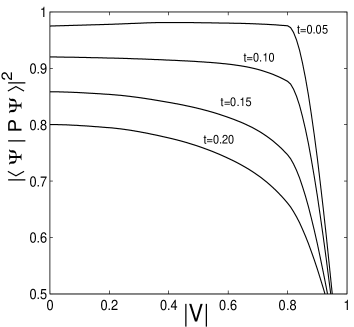
Figure 1: Projection of the exact ground state onto the one corresponding to the limit $U\to\infty$ as a function of $|V|/U$ for $N=6$, $M=8$, and different values of $t/U$.

To illustrate these behaviors we present now numerical exact results for a system of $N=6$ bosons and $V<0$. Even though this is a small number, this may closely represent some experimental situations with atomic systems Bloch where the effective number of atoms in the 1D lattice may be relatively small. Given that Hamiltonian (1) is invariant under global spin rotations, we diagonalize it within subspaces of fixed total spin, $S$, and fixed $z$ component of the spin, $S_{z}$. In order to to check the “fermionization scheme” we show in Fig. 1 the projection of the exact ground state of the system on the one calculated with the projected Hamiltonian, as a function of the strength of the attraction, $|V|$. In agreement with the predictions, when $t\ll U$ and as far as $|V|<U$ the overlap is more than $95\%$ . However, as we approximate the limit $|V|=U$, or as $t$ is increased, the system looses the fermionic character.

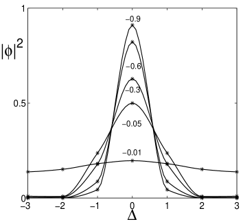
Figure 2: $|\varphi|^{2}$ as a function of $\Delta/U$ for the variational wave function (5) and for $N=6$, $t=0.1U$ and different values of $|V|/U$.

For a regime of parameters in which the fermionization is valid, we can use the variational wave function (5) to understand the nature of the bosonic pairs. Figure 2 shows the probability density of the pair, $|\varphi|^{2}$, corresponding to the variational state (5). We clearly see how the nature of the pair exhibits a smooth crossover from being delocalized, for $|V|\ll t$ to get localize at $\Delta=0$ for $|V|\gg t$. The gap for spin excitations, given by the expression $\delta=(E_{N-1}-2E_{N}+E_{N+1})/2$ Lieb , is plotted in Fig. 3 as a function of $|V|$. As the attraction increases the energy required to break a pair increases. The behavior of the gap near $|V|=U$ is due to the transition from a paired state to the “big boson” state.

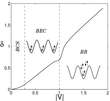
Figure 3: Gap for spin excitations, $\delta/U$, as a function of $|V|/U$ for $N=6$, and $t=0.1U$. The three regimes are indicated in the figure.

The existence of pairs and the smooth evolution from Cooper pairs to localized pairs can be detected by analyzing the response of the system to a (Raman) laser that couples the internal states of the atoms, so that $H_{B}=H+B\sum_{i=1}^{M}a^{\dagger}_{i\uparrow}\,a_{i\downarrow}+a^{\dagger}_{i\downarrow}\,a_{i\uparrow}$, where the parameter $B$ can be varied by tuning the intensity of the laser. The effect of this laser can be understood as follows. Let us assume that the system is in a paired state with pair wave function $\varphi(x)(|\uparrow\downarrow\rangle+|\downarrow\uparrow\rangle)$. The laser will try to rotate the spin state into the state $|\uparrow\uparrow\rangle+|\downarrow\downarrow\rangle$. Since this rotation must break the pair it follows that the response will be very low until a value $B\sim\delta$ is reached. Thus, $\delta$ can be detected by observing, for instance, the fluctuations induced in the the $z$ component of the total spin, $\langle S_{z}^{2}\rangle$, as a function of $B$, as it is illustrated in Fig. 4. As predicted, the system response, quantified by $\left.d^{2}\langle S_{z}^{2}\rangle/dB^{2}\right|_{B=0}$, is extremely large for $V=0$, when we have no pairs and the system holds no resistance to be rotated, and decreases monotonically for increasing attraction, revealing the existence of pairs. Note that for $|V|\gg t$, rotation of the on-site pair will imply exciting the system out of the subspace spanned by (2), since two atoms with the same spin will be left on the same site, and therefore excitation will occur for $B\gtrsim U$.

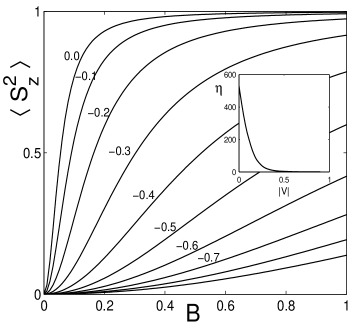
Figure 4: $\langle S_{z}^{2}\rangle$ as a function of $B/U$, for $N=6$, $t=0.1U$, and different values of $V/U$. The inset shows the second derivative, $\eta$, of $\langle S_{z}^{2}\rangle$ with respect to $B$ (in units of $U$) at zero magnetic field, as a function of $|V|/U$.

In summary, we have shown that with the experiments that are being carried out with bosons in optical lattices one can observe a great variety of fermionic correlation phenomena, including Cooper pair formation and spin–density separation. These atomic systems may be simpler to manipulate than fermions themselves and can provide a very clean laboratory to study several interesting phenomena which have eluded observation so far. Apart from that, the system proposed here may bring up novel phenomena in 2 and 3D optical lattices. Even though the Jordan–Wigner transformation is not appropriate, some of the phenomena predicted for Fermions (like d-wave pairing or an analogue) may appear in the case of bosons in the regime $U>|V|$, and therefore these cases are worth exploring both theoretically and experimentally.

Discussions with I. Bloch, J. von Delft, C. Tejedor, and P. Zoller are gratefully acknowledged. B. P. is indebted to G. Gómez-Santos for illuminating discussions.

References

- (1) See, for example, Nature 416, 206 (2002).
- (2) H. T. C. Stoof, M. Houbiers, C. A. Sackett, R. G. Hulet, Phys. Rev. Lett. 76, 10 (1996); M. Houbiers et al., Phys. Rev. A 56, 4864 (1997).
- (3) B. DeMarco and D. S. Jin, Science 285, 1703 (1999); F. Schreck, L. Khaykovich, K. L. Corwin, G. Ferrari, T. Bourdel, J. Cubizolles, C. Salomon, Phys. Rev. Lett. 87, 080403 (2001); G. Truscott, K. E. Strecker, W. I. McAlexander, G. B. Partridge, R. G. Hulet, Science 291, 2570 (2001); Z. Hadzibabic, C. A. Stan, K. Dieckmann, S. Gupta, M. W. Zwierlein, A. Görlitz, W. Ketterle, cond-mat/0112425; G. Roati, F. Riboli, G. Modugno, and M. Inguscio, cond-mat/0205015.
- (4) M. Holland, S. J. J. M. F. Kokkelmans, M. L. Chiofalo, R. Walser, Phys. Rev. Lett. 87, 120406 (2001); Y. Ohashi, A. Griffin, cond-mat/0201262; W. Hofstetter, J.I. Cirac, P. Zoller, E. Demler, and M.D. Lukin, cond-mat/0204237.
- (5) M. Greiner O. Mandel, T. Esslinger, Th. W. Hänsch, I. Bloch, Nature 415, 39 (2002).
- (6) D. Jaksch, C. Bruder, J. I. Cirac, C. W. Gardiner, P. Zoller, Phys. Rev. Lett. 81, 3108 (1998).
- (7) M. Girardeau, Journal of Math. Phys. vol.1, 6, 516 (1960); M. Girardeau, Phys. Rev. 139 2B, 500 (1965); Bogoliubov, Korepin, Izergin, in Quantum Inverse Scattering Method and correlation functions (Cambridge University Press, 1993).
- (8) B. Paredes, P. Fedichev, J. I. Cirac, P. Zoller, Phys. Rev. Lett. 87, 10402 (2001); B. Paredes, P. Zoller, J. I. Cirac, cond-mat/0203061.
- (9) The only requirement is that the interaction constant between the same internal levels is larger than the one between different ones. For simplicity we have assumed that both internal levels have identical interactions, as it would be the case for the states of the hyperfine manifold. Note also that in this regime no three body loses can occur, since there are never three atoms in the same site.
- (10) Depending on whether and are even or odd, the bosonic Hamiltonian maps to a Hubbard chain with periodic or antiperiodic boundary conditions (E. Lieb, W. Liniger, Phys. Rev. 130-4, 1605 (1963)). For simplicity, will assume here that , odd. Clearly, for sufficiently large, this assumption does not restrict our conclusions.
- (11) See, e.g., S. Sachdev, in Quantum Phase Transitions, (Cambridge University Press, 1999)
- (12) The Hubbard model. Recent results., edite By M. Rasetti (World Scientific, 1991); The Hubbard model. A reprint volume, edited by A. Motorsi (World Scientific, 1992).
- (13) F. D. M. Haldane, J. Phys. C 14, 2585 (1981).
- (14) P. Nozieres, S. Schmitt-Rink, J. Low Temp. Phys. 59, 195 (1985); D. M. Eagles, Phys. Rev. 186, 456 (1969); A. J. Leggett, in Modern Trends in the Theory of Condensed Matter, edited by A. Pekalski and J. Przystawa (Springer, Berlin, 1980). M. Randeira, in Bose-Einstein condensation, edited by A. Griffin, D. W. Snoke, and S. Stringari (Cambridge University Press, 1995).
- (15) A. Recati, P. O. Fedichev, W. Zwerger, P. Zoller, cond-mat/0206424.
- (16) See, for example, P. Fulde in Electron correlations in molecules and solids, (Springer, Berlin, 1995).
- (17) K. Tanaka and F. Marsiglio Phys. Rev. B 60, 3508 (1999).
- (18) E. H. Lieb, F. Y. Wu, Phys. Rev. Lett. 20, 1445 (1968).