Computational complexity arising from degree correlations in networks

Abstract

We apply a Bethe-Peierls approach to statistical-mechanics models defined on random networks of arbitrary degree distribution and arbitrary correlations between the degrees of neighboring vertices. Using the NP-hard optimization problem of finding minimal vertex covers on these graphs, we show that such correlations may lead to a qualitatively different solution structure as compared to uncorrelated networks. This results in a higher complexity of the network in a computational sense: Simple heuristic algorithms fail to find a minimal vertex cover in the highly correlated case, whereas uncorrelated networks seem to be simple from the point of view of combinatorial optimization.

The last few years have seen a great advance in the study of complex networks albert02 , where the term complex refers to the existence of one or more of the following properties: small world effect watts98 , power-law degree distribution albert02 , and more recently also correlations redner ; pastor01 ; berg ; newman02 . On the other hand, if we focus on the solution of a given task on top of these networks, the term complex is better associated with the time required to solve it, i.e. with its computational complexity garey79 . In this context, a problem is complex if its algorithmic solution time is growing exponentially in the network size. At the core of complex optimization problems one finds the NP-hard class garey79 , where NP stands for non-deterministic polynomial time.

In the case of uncorrelated networks with power law degree distributions we can take profit of the existence of hubs to solve different problems, like destroying the giant component percolation , preventing epidemic outbreaks spreading , and searching searching . The extremely inhomogeneous structure of uncorrelated networks can also be exploited to approximate or even to solve instances of NP-hard problems using heuristic algorithms running in polynomial time. However, the influence of properties like degree correlations or clustering is not clear yet. Recent studies of percolation newman02 and disease spreading boguna02 have shown that degree correlations can quantitatively change, e.g., the transition threshold but qualitatively the results are similar to those obtained for uncorrelated networks.

This changes drastically if we consider hard optimization tasks defined over correlated networks. In this work we study the influence of degree correlations on the computational complexity, and in a more general perspective the relation between the topology of complex networks and the computational complexity of hard problems defined on top of them. For this purpose we generalize the Bethe-Peierls approach to statistical-mechanics models defined on networks with an arbitrary degree distribution and arbitrary degree correlations of adjacent nodes.

The approach is applied to characterize the minimal vertex covers on these graphs. We have chosen this problem for two reasons: It belongs to the basic NP-hard optimization problems over graphs garey79 , and has found applications in monitoring Internet traffic breitbart and denial of service attack prevention park . Our analytical results are later compared with an approximate solution obtained using a heuristic algorithm. This heuristic fails to find minimal vertex covers in the strongly correlated case, whereas networks with low correlations seem to be simple from the point of view of combinatorial optimization. Within our analytical approach, this change of behavior is associated with replica symmetry breaking (RSB).

Consider the set of undirected graphs with $N$ vertices and arbitrary degree distribution $p_{d}$. Following a randomly chosen edge, we will find a vertex of degree $d+1$ with probability $q_{d}=(d+1)p_{d+1}/c$, with $c$ denoting the average degree. The number $d$ of additional edges will be called excess degree. We further assume correlations between adjacent vertices: The probability that a randomly chosen edge connects two vertices of excess degrees $d,d^{\prime}$ is given by $(2-\delta_{d,d^{\prime}})e_{dd^{\prime}}$. The conditional probability that a vertex of excess degree $d$ is reached following any edge coming from a vertex of excess degree $d^{\prime}$,

$$p(d|d^{\prime})=e_{dd^{\prime}}/q_{d^{\prime}}\ ,$$ (1)

thus explicitly depends on both $d$ and $d^{\prime}$. Consistency with the degree distribution requires $\sum_{d^{\prime}=0}^{\infty}e_{dd^{\prime}}=q_{d}$, and $e_{dd^{\prime}}$ has to be symmetric. For uncorrelated graphs $e_{dd^{\prime}}=q_{d}q_{d^{\prime}}$ factorizes. The strongest positive correlations are reached for $e_{dd^{\prime}}=q_{d}\delta_{dd^{\prime}}$ where only vertices of equal degrees are connected.

Let us now consider a general statistical-mechanics model with discrete degrees of freedom defined on vertices, and interactions defined on edges. We use a lattice gas model described by the Hamiltonian

$$-\beta H=\sum_{i<j}J_{ij}w(x_{i},x_{j})+\mu\sum_{i}x_{i}$$ (2)

defined for any microscopic configuration $x_{i}=0,1,\ i=1,...,N$. $J$ is the adjacency matrix with entries $J_{ij}=1$ if vertices $i$ and $j$ are adjacent, and $J_{ij}=0$ else. The inverse temperature is denoted by $\beta$, the chemical potential by $\mu$. The interactions $w(x_{i},x_{j})$ are arbitrary, thus including also the case of the ferromagnetic Ising model, $w(x_{i},x_{j})=(2x_{i}-1)(2x_{j}-1)$. The only disorder present in Eq. (2) is given by the edges $J_{ij}$. Generalizations to disordered interactions, as present e.g. in spin-glasses, random local fields or non-binary discrete variables are evident. For clarity of the presentation, we restrict ourselves to the simple model given above.

Since the graphs are locally tree-like, the model can be solved by the iterative Bethe-Peierls scheme which becomes exact if only one pure state is present. The free energy can be expressed in terms of simple effective-field distributions acting on vertices of given degree. In the case of multiple pure states this has to be generalized to the cavity approach, see e.g. MePa for the example of a spin-glass on a Bethe lattice of constant vertex degree. Alternatively, one can apply the replica approach. The simple Bethe-Peierls solution corresponds to the assumption of replica symmetry (RS), whereas the full cavity approach is able to handle also the case of RSB.

Take any edge $(i,j)$, i.e. $J_{ij}=1$. Let us introduce $Z_{x}^{(i|j)}$ as the partition function of the subtree rooted in $i$, with deleted edge $(i,j)$, and with $x_{i}$ fixed to the value $x$. This partition function can be calculated iteratively,

$$Z_{0}^{(i|j)} = \prod_{k\neq j|\ J_{ik}=1}\left(e^{w(0,0)}Z_{0}^{(k|i)}+e^{w(0,1)}Z_{1}^{(k|i)}\right)$$ (3)

$$Z_{1}^{(i|j)} = e^{\mu}\prod_{k\neq j|\ J_{ik}=1}\left(e^{w(1,0)}Z_{0}^{(k|i)}+e^{w(1,1)}Z_{1}^{(k|i)}\right)$$

The effective fields $h_{(i|j)}=\ln(Z_{1}^{(i|j)}/Z_{0}^{(i|j)})$ are thus determined by the iterative description

$$h_{(i|j)}=\mu+\sum_{k\neq j|\ J_{ik}=1}u(h_{(k|i)})\ .$$ (4)

where $u(h_{(k|i)})$ is the effective field induced by $x_{k}$ on site $i$, and is given by

$$u(h_{(k|i)})=\ln\left(\frac{e^{w(1,0)}+e^{w(1,1)+h_{(k|i)}}}{e^{w(0,0)}+e^{w(0,1)+h_{(k|i)}}}\right)\ .$$ (5)

The free energy of the system can be written as

$$-\beta Nf=\sum_{i}f_{i}+\sum_{i<j}J_{ij}(f_{ij}-f_{i}-f_{j})$$ (6)

where the link contribution equals

$$f_{ij}=-\ln\left(\sum_{x_{i},x_{j}}e^{w(x_{i},x_{j})+h_{(i|j)}x_{i}+h_{(j|i)}x_{j}}\right)\ ,$$ (7)

whereas the site contribution

$$f_{i}=-\ln\left(\sum_{x_{i}}e^{h_{i}x_{i}}\right)$$ (8)

depends on the cavity field

$$h_{i}=\mu+\sum_{k|\ J_{ik}=1}u(h_{(k|i)})$$ (9)

resulting from the influence of all neighbors on vertex $i$.

Let us now assume, that the model has only one pure state, which corresponds to the assumption of RS. In this case, the iterative procedure given by Eq. (4) converges to well-defined distributions $P_{d}(h)$ of effective fields $h_{(i|j)}$ restricted to vertices of excess degree $d$. They are determined by the self-consistency equation

$$P_{d}(h) = \int_{-\infty}^{\infty}\prod_{l=1}^{d}\left(dh_{l}\sum_{d_{l}=0}^{\infty}p(d_{l}|d)P_{d_{l}}(h_{l})\right)$$ (10)

$$\times\delta\left(h-\mu-\sum_{l=1}^{d}u(h_{l})\right)\ .$$

Please note that, in contrast to the uncorrelated case, we do need the field distributions for all possible excess degrees. In the uncorrelated case, the average of these distributions over $q_{d}$ is sufficient. We may also introduce the analogous distributions $\tilde{P}_{d}(h)$ of cavity fields $h_{i}$ for vertices of given degree $d$ (note: here the full degree is relevant), they can be calculated from $P_{d}(h)$ by

$$\tilde{P}_{d}(h) = \int_{-\infty}^{\infty}\prod_{l=1}^{d}\left(dh_{l}\sum_{d_{l}=0}^{\infty}p(d_{l}|d-1)P_{d_{l}}(h_{l})\right)$$ (11)

$$\times\delta\left(h-\mu-\sum_{l=1}^{d}u(h_{l})\right)\ .$$

Replacing the sum over vertices and edges in Eq. (6) by the corresponding averages over $P_{d}(h)$ resp. $\tilde{P}_{d}(h)$, we finally find the free-energy density

$$\beta f = -\sum_{d=0}^{\infty}(d-1)\ p_{d}\ \int_{-\infty}^{\infty}dh\ \tilde{P}_{d}(h)\ln\left(1+e^{h}\right)$$

$$+\frac{c}{2}\sum_{d,d^{\prime}=0}^{\infty}e_{dd^{\prime}}\int_{-\infty}^{\infty}dh\ dh^{\prime}P_{d}(h)P_{d^{\prime}}(h^{\prime})$$

$$\ln(e^{w(0,0)}+e^{w(1,0)+h}+e^{w(0,1)+h^{\prime}}+e^{w(1,1)+h+h^{\prime}})$$

The simplest application of this approach is given by the ferromagnetic Ising model. If we look to the ground-states, i.e. to the limit $\beta\to\infty$, we find that, as to be expected, the global magnetization is determined by the size of the giant component. The existence of a ferromagnetic phase at low temperature is thus related to percolation. The latter was already analyzed in Ref. newman02 .

Another application is given by the vertex cover (VC) problem. It belongs to the basic NP-hard optimization problems garey79 and, therefore, it is expected to require a solution time which is growing exponentially with the graph size. Let us be more precise. Given a graph with vertices $i\in\{1,...,N\}$ and edges $\{(i,j)|1\leq i<j\leq N,J_{ij}=1\}$, a vertex cover $V$ is a subset of vertices, $V\subset\{1,...,N\}$, such that at least one end-vertex of every edge is contained in $V$. So no edge $(i,j)$ is allowed to exist with $i\notin V$ and $j\notin V$. Of course, the set of all vertices forms a trivial VC. The hard optimization problem consists in finding the minimal VC.

Using the hard-sphere lattice-gas representation introduced in WeHa , where $x_{i}=1$ if $i\notin V$, and $x_{i}=0$ if $i\in V$, the VC condition can be rewritten as

$$\prod_{(i,j)|J_{ij}=1}(1-x_{i}x_{j})=1$$ (13)

which fits into the above framework by setting $e^{w(x_{i},x_{j})}=1-x_{i}x_{j}$. The chemical potential can be used to fix the cardinality of the VC, minimal ones are obtained in the limit $\mu\to\infty$. They correspond to maximal packings in the lattice-gas picture. To perform the limit $\mu\to\infty$ all fields have to be rescaled as $h=\mu z$ WeHa . We obtain

$$P_{d}(z) = \int_{-\infty}^{\infty}\prod_{l=1}^{d}\left(dz_{l}\sum_{d_{l}=0}^{\infty}p(d_{l}|d)P_{d_{l}}(z_{l})\right)$$ (14)

$$\times\delta\left(z-1-\sum_{l=1}^{d}\max(0,z_{l})\right)\ ,$$

which is solved by $P_{d}(z)=\sum_{l=-1}^{+\infty}\rho_{l}^{(d)}\delta(z+l)$. This ansatz allows for integer valued fields only, we find a simple relation including only the $\rho_{-1}^{(d)}$:

$$\rho_{-1}^{(d)}=\left[\sum_{d_{1}=0}^{\infty}p(d_{1}|d)(1-\rho_{-1}^{(d_{1})})\right]^{d}$$ (15)

All other $\rho_{l}^{(d)}$ follow easily. The expression inside the parenthesis can be understood as the average probability $\pi_{d}$ that an edge entering a vertex of degree $d+1$ carries a constraint, i.e. that it is not yet covered by the neighboring vertex. It thus fulfills the condition

$$\pi_{d}=\sum_{d_{1}=0}^{\infty}p(d_{1}|d)(1-\pi_{d_{1}})^{d_{1}}\ .$$ (16)

Having in mind that, due to the limit $\mu\to\infty$, every vertex with positive $z$ is fixed to $x=1$, every one with negative $z$ has $x=0$, we can immediately read off the fraction of vertices belonging to a minimal VC,

$$x_{c}=1-\sum_{d=0}^{\infty}p_{d}(1-\pi_{d-1})^{d-1}\left(1+\frac{d-2}{2}\pi_{d-1}\right)\ .$$ (17)

Remember that the last expressions are related to the validity of RS, i.e. to the existence of a single connected cluster of minimal VCs in configuration space. As observed in WeHa , RS is related to the local stability of this solution. In presence of RSB, Eq. (16) has no stable solution. Since it has to be solved by numerical iteration in the general case, an instability prevents the program from convergence and thus provides a precise tool to detect RSB without any RSB calculation.

To see how this works out, we concentrate on networks having equal degree distributions but different correlation properties. We restrict our attention to scale-free graphs with $p_{d}\sim d^{-\gamma}$ for $d=1,...,\infty$, with $\gamma>2$. For vertex cover, interesting effects are expected to appear for positive correlations, or assortative networks. We therefore consider

$$e_{dd^{\prime}}=q_{d}\left[r\delta_{d,d^{\prime}}+(1-r)q_{d^{\prime}}\right]\ .$$ (18)

For $0\leq r\leq 1$, this expression linearly interpolates between uncorrelated ($r=0$) and fully assorted ($r=1$) networks. Please note that this network is percolated for all $\gamma$ as soon as $r>0$. In Fig. 1 we show the resulting size of the minimal VCs for different values of $\gamma$ as a function of $r$. The RS solution breaks at a certain value of $r$ that depends on $\gamma$. There, the solution-space structure changes drastically, from being unstructured, or RS, in the low correlated case to being clustered, or RSB, for sufficiently high correlations.

To check the consequences of this transition for heuristic optimization algorithms, we have numerically generated scale-free networks with correlations (18), and applied a generalization of the leaf-removal heuristic of Bauer and Golinelli bauer01 . For the special case of correlations given by Eq. (18), the network can be generated using a modification of the Molloy-Reed algorithm MoRe for random graphs of arbitrary degree distribution. First, each node $i$ is assigned a degree $d_{i}$ with probability $p_{d_{i}}$. Then we create a set ${\cal L}$ containing $d_{i}$ copies of each node $i$. Finally, pairs of nodes are connected according to following rule: (i) Select a node $i$ in ${\cal L}$ at random. (ii) With probability $r$, select a second node $j\in{\cal L}$ with $d_{j}=d_{i}$ in ${\cal L}$ at random; otherwise select an arbitrary node $j\in{\cal L}$ at random. (iii) Connect $i$ and $j$ and delete both from ${\cal L}$. This is repeated until ${\cal L}$ is empty.

Once the network is generated, we construct a VC using a generalized leaf-removal algorithm weigt02 defined as follows: Select a vertex of minimal current degree from the network and cover all its neighbors. The considered vertices and all incident edges are removed from the network. This step is iterated untill the full network is removed. If, for some graph, this algorithm stops without having ever chosen vertices of current degree $d\geq 2$, the constructed VC is minimal bauer01 . Overestimations may appear if the algorithm is forced to select also vertices of higher degree $d\geq 2$, where the error can be at most $d-1$. Thus, summing $(d-1)(1-\delta_{d,0})/N$ over all iteration steps, we get an upper bound $\Delta x$ on the total error made in estimating $x_{c}$ using the above heuristic algorithm. If $\Delta x$ goes to zero in the large-$N$ limit, the algorithm has consequently constructed an almost minimal VC.

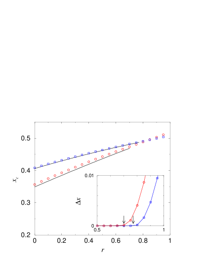
Figure 1: Minimal VC size for a network with degree distribution $p_{d}\sim d^{-\gamma}$ and degree correlations given by Eq. (18). The lines give the analytical solution for $\gamma=2.5$ (lower curve) and $\gamma=3.0$ (upper curve). The curves stop at the point where RS breaks. The symbols are numerical estimates for $\gamma=2.5$ (circles) and $\gamma=3.0$ (squares), and network size $N=10^{6}$. In the inset we plot the upper error bound $\Delta x$ for generalized leaf removal. The onset of non-zero error coincides with the RSB transition, marked by arrows.

In Fig. 1 we show the size of VCs found by generalized leaf removal as a function of $r$. Up to the RSB point the numerical solutions are close to the analytical values, up to finite-size corrections resulting mainly from a degree cutoff $d_{max}\sim N^{1/\gamma}$. Beyond the RSB point we still have a numerical estimate but we cannot be sure that it is optimal. In the inset of Fig. 1 the upper bound on the error is displayed. In the RS region we have $\Delta x\approx 0$ for $N\gg 1$ and, therefore, the heuristic algorithm asymptotically yields the exact value $x_{c}$. However, in the highly correlated region we find a finite $\Delta x$ at any network size, thus the heuristic algorithm fails to find almost minimal vertex covers. Moreover, the point where $\Delta x$ becomes different from zero coincides with the RSB point.

It is interesting to know in which phase realistic networks are. VCs have found applications in monitoring the Internet traffic breitbart and in denial of service attack prevention park . The analysis of Internet maps has revealed negative (dissasortative) correlations at the autonomous system level pastor01 . Negative correlations are actually common in technological and biological networks newman02 . Hence, the generalized leaf-removal heuristic should output almost optimal VCs in linear time. On the contrary, social networks exhibit positive (assortative) correlations newman02 . In this case VCs can be used to monitor social relations between pairs of individuals but, because of the existence of positive correlations, simple heuristic algorithms may fail to produce near optimal solutions.

To summarize, we have generalized the Bethe-Peierls approach to random networks with degree correlations and analyzed the VC problem as a prototype optimization problem defined over graphs. We have found that uncorrelated power-law networks are simple from the point of view of combinatorial optimization, inhomogeneities of neighboring vertices can be exploited. The introduction of sufficiently large degree correlations leads to RSB and thus to a failure of simple heuristic algorithms. For constructing optimal solutions, complete algorithms including e.g. backtracking have to be used. These, however, result in general in exponential solution times, and thus in a higher algorithmic complexity. Our results point out that optimization problems in many technological and biological networks can be simple due to the strong degree inhomogeneities and negative correlations present on them.

- (1) R. Albert and A.-L. Barabási, Rev. Mod. Phys. 74, 47 (2002); S.N. Dorogovtsev and J.F.F. Mendes, Adv. Phys. 51, 1079 (2002).
- (2) D. J. Watts and S. H. Strogatz, Nature 393, 440 (1998).
- (3) P.L. Krapivsky and S. Redner, Phys. Rev. E 63, 066123 (2001);
- (4) R. Pastor-Satorras, A. Vázquez, and A. Vespignani, Phys. Rev. Lett. 87, 258701 (2001); A. Vázquez, R. Pastor-Satorras, and A. Vespignani, Phys. Rev. E 65, 066130 (2002).
- (5) J. Berg and M. Lässig, Phys. Rev. Lett. 89, 228701 (2002).
- (6) M. E. J. Newman, Phys. Rev. Lett. 89, 208701 (2002).
- (7) M. Garey and D. Johnson, Computers and Intractability: A Guide to the theory of NP-completeness (Freeman, San Francisco, 1979).
- (8) R. A. Albert, H. Jeong, and A.-L. Barabási, Nature 406, 378 (2000); D. S. Callaway, M. E. J. Newman, S. H. Strogatz, and D. J. Watts, Phys. Rev. Lett. 85, 5468 (2000); R. Cohen, K. Erez, D. ben-Avraham, and S. Havlin, Phys. Rev. Lett. 86, 3682 (2001).
- (9) R. Pastor-Satorras and A. Vespignani, Phys. Rev. Lett. 86, 3200 (2001); Phys. Rev. E 65, 036104 (2002).
- (10) L. A. Adamic, R. M. Lukose, A. R. Puniyani, B. A. Huberman, Phys. Rev. E 64, 046135 (2001).
- (11) M. Boguña and R. Pastor-Satorras, Phys. Rev. E, 66, 047104 (2002).
- (12) Y. Breitbart, C.-Y. Chan, M. Garofalakis, R. Rastogi, and A. Silverschatz, Proceedings of IEEE INFOCOM (Alaska, USA, 2001).
- (13) K. Park and H. Lee, Proceedings of ACM SIGCOMM (California, USA, 2001).
- (14) M. Molloy and B. Reed, Random Struct. and Algorithms 6, 161 (1995); M.E.J. Newman, S.H. Strogatz, and D.J. Watts, Phys. Rev. E 64, 026118 (2001).
- (15) M. Mézard and G. Parisi, Eur. Phys. J. B 20, 217 (2001).
- (16) M. Weigt and A. K. Hartmann, Phys. Rev. Lett. 84, 6118 (2000); Phys. Rev. E 63, 56127 (2001).
- (17) M. Bauer, O. Golinelli, Eur. Phys. J. B 24, 339 (2001).
- (18) M. Weigt, Eur. Phys. J. 28, 369 (2002).