Uncorrelated Random Networks

Abstract

We define a statistical ensemble of non-degenerate graphs, i.e. graphs without multiple- and self-connections between nodes. The node degree distribution is arbitrary, but the nodes are assumed to be uncorrelated. This completes our earlier publication bck , where trees and degenerate graphs were considered. An efficient algorithm generating non-degenerate graphs is constructed. The corresponding computer code is available on request. Finite-size effects in scale-free graphs, i.e. those where the tail of the degree distribution falls like $n^{-\beta}$, are carefully studied. We find that in the absence of dynamical inter-node correlations the degree distribution is cut at a degree value scaling like $N^{\gamma}$, with $\gamma=\min[1/2,1/(\beta-1)]$, where $N$ is the total number of nodes. The consequence is that, independently of any specific model, the inter-node correlations seem to be a necessary ingredient of the physics of scale-free networks observed in nature.
PACS number(s): 05.10.-a, 05.40.-a, 87.18.Sn
LPT Orsay 02/64

I Introduction

This paper is a direct continuation of ref. bck . The importance of defining statistical ensembles of random graphs in order to understand the geometry of wide classes of networks independently of any specific model was emphasized there. Concepts borrowed from field theory were used to define the ensemble of uncorrelated graphs and an algorithm generating such graphs was proposed. The general philosophy of our approach was illustrated by focusing on a graph sub-ensemble, namely on an ensemble of connected trees with a scale-free degree distribution, where a number of hopefully interesting analytic results could be presented. But it should have been obvious that the adopted framework is of much broader applicability. Actually, we have explicitly stated that our algorithm generates efficiently not only trees, but also so-called pseudographs, called degenerate graphs in bck . However, we have also indicated that we have encountered problems dealing with simple (i.e. non-degenerate) graphs. Hence the discussion of these non-degenerate graphs was postponed. We are now returning to the problem of defining the statistical ensembles of networks, which in the meantime has attracted the attention of other researchers dms -bb (at this point is it fair to mention also ref. nsw , an early paper on uncorrelated graphs).

Although some overlap with bck is unavoidable, if this paper is to be self-contained, we would like to reduce the overlap to a minimum. The reader is invited to consult bck when he finds the discussion of this paper too sketchy.

We shall not dwell much in introducing the subject. Let us recall that a graph is just a collection of nodes (vertices) connected by links (edges). It is a mathematical idealization representing the various networks one encounters in nature, in social life, in engineering, etc. Quite often the pattern of connections between nodes looks fairly random. The concept of a random graph emerges quite naturally.

Random graphs are interesting in themselves. There exists a classical theory of random graphs, a beautiful piece of pure mathematics er . It turns out, however, that most large graphs one encounters in applications are not covered by this theory. The access - relatively recent - to the corresponding data triggered a rather intense activity (see the refs. rev1 ; rev2 and references therein).

Networks are also interesting considered from a broader perspective: it is useful to represent the architecture, so to say the skeleton of many complex systems by an appropriate network. Hence, graphs are in a sense a gateway to the theory of complex systems, an exciting and promising new direction of research.

The plan of this paper is as follows: In Sect. II we recall the definition of the ensemble of uncorrelated random graphs and we discuss the algorithm generating the graphs. In Sect. III we present the results of a sample of computer simulations, aimed to help understanding finite-size effects. The latter play a very important role as soon as the degree distribution has a fat tail. We explain the behavior of the data using an analytic argument. We conclude in Sect. IV. For definiteness, we consider undirected graphs only, as in bck .

II Defining the ensemble

Let us recall the construction proposed in ref. bck . The partition function for the ensemble of random graphs is written as the formal integral defining a minifield theory

$$Z=\int_{-\infty}^{+\infty}\text{d}\phi\exp{\frac{1}{\kappa}[-\phi^{2}/2\lambda+g\sum_{n=1}^{\infty}p_{n}\phi^{n}]}$$ (1)

It will be seen that the non-negative constants $p_{n}$ correspond to the degree distribution, while the auxiliary constants $g$, $\lambda$ and $\kappa$ control the dependence of $Z$ on the number of nodes, links and loops, repectively. The integral does not exist, but $Z$ can be treated formally as a generating function in the Gaussian perturbation theory. The main idea is to expand the exponential under the integral in (1) in powers of $g$ :

$$Z=\int\text{d}\phi\;\exp{\frac{1}{\kappa}[-\phi^{2}/2\lambda]}\;[1+\frac{g}{\kappa}\sum_{n}p_{n}\phi^{n}$$

$$+\frac{1}{2!}(\frac{g}{\kappa})^{2}\sum_{n,m}p_{n}p_{m}\phi^{n+m}+\dots]$$ (2)

to get a series in $g$ with well defined coefficients, viz. integrals with the Gaussian measure of integer powers of $\phi$. Each such integral is equal to a sum of contributions, which can be represented graphically by the so-called Feynman diagrams fieldth . We have explained in ref. bck how such a diagram emerges, using a particular example. We do not have enough space to develop the point in more details. For those readers who are not conversant with field theory techniques we list the rules for constructing and calculating the Feynman diagrams corresponding to the term of order $O(g^{N})$ in (2):

Each diagram has $N$ labeled nodes. One should draw all topologically distinct diagrams, distributing degrees among nodes in all possible manners and connecting nodes pairwise. Self- and multiple-connections between nodes are allowed. Notice the similarity with the Molloy-Reed construction mr . With each diagram is associated a number, called the Feynman amplitude, determined by the following rules: each node of degree $n$ contributes a factor $\frac{g}{\kappa}p_{n}n!$ and each link contributes a factor $\kappa\lambda$. There is a symmetry factor $1/2$ associated with every line connecting a node to itself and a symmetry factor $1/m!$ associated with every m-tuple connection between nodes foot5 . There is also a factor $Z_{0}/N!$, the factorial being a remnant of the expansion of an exponential and $Z_{0}$ being the value of the Gaussian integral.

Finally, the series representation of the partition function reads

$$Z=Z_{0}\sum_{L,N}\frac{g^{N}}{N!}\kappa^{L-N}\lambda^{L}\sum_{D}\frac{1}{S(D)}\prod_{j=1}^{N}p_{n_{j}}n_{j}!$$ (3)

where one sums over labeled diagrams $D$ having a fixed numer of nodes and links, respectively $N$ and $L$. $S(D)$ is the product of factors 2 and factorials associated with self- and multiple-connections and $n_{j}$ is the degree of the $j^{\text{th}}$ node. One can show that the analogous series for $\log Z$ receives contributions of connected diagrams only. In this case the expansion in powers of $\kappa$ is a loop expansion: the leading term corresponds to $L=N+1$ and comes from tree diagrams, the next term comes from one-loop diagrams etc.

Our idea is to identify the Feynman diagrams of the toy model defined by eq. (1) with the graphs of a statistical ensemble. Indeed, Feynman diagrams are identical to graphs familiar to network community people, except that there are definite rules to calculate the corresponding weights. The minifield formulation enables one to summarize compactly the content of the model and has also the advantage of being a good starting point for analytical calculations, like those of ref. bck .

In the following, we always work with graph ensembles where $N$ and $L$ are fixed. Hence, up to an irrelevant factor, the weight $w$ of a labeled graph that is non-degenerate, i.e. such that nodes are neither multiply connected nor connected to themselves, is just

$$w\sim\prod_{j=1}^{N}\;p_{n_{j}}n_{j}!$$ (4)

In the presence of degeneracies one has to multiply the r.h.s. (right hand side) of (4) by the factor $S^{-1}$ appearing in (3).

Eq. (4) gives the weight of a microstate. Notice the factorized form and therefore the absence of non-trivial, dynamical correlations. Notice also that with the choice $p_{n}\propto(\text{const})^{n}/n!$ all non-degenerate graphs with the same $N$ and $L$ are equiprobable, because

$$\sum_{j}n_{j}=2L$$ (5)

Thus, with a Poissonian $p_{n}$ one recovers the classical graph ensemble of Erdös and Rényi. The ensemble under discussion is the most conservative generalization of the classical ensemble to the case of an arbitrary degree distribution.

At this point the statistical ensemble is basically defined. However, in this paper, we wish to focus on non-degenerate graphs, which are the primary objects in graph theory. They correspond to a sub-ensemble of Feynman diagrams. In the conventional applications of field theory no specific recipe is formulated to single these diagrams out. Such a recipe is, however, needed here. Otherwise our definition of the ensemble would be too vague to be useful in applications.

Before going farther let us outline the strategy we shall follow: as stated above our goal is now to complete the definition of the ensemble by the construction of an algorithm generating non-degenerate graphs. But we do not achieve this goal directly. First we construct, following ref bck , an algorithm generating graphs that are degenerate. Then, we show that the ensemble of these degenerate graphs is isomorphic, as far as the degree distribution is concerned, to the known model of balls-in-boxes binb . Using this mapping of one model on another we conclude that asymptotically the degree distribution $P_{n}$ in the ensemble of degenerate graphs is just $p_{n}$ : $P_{n}\to p_{n}$ for $N\to\infty$. Since we suspect that in this limit the degree distributions are the same for degenerate and non-degenerate graphs, we impose the appropriate constraint on the algorithm and perform a sample of computer experiments, to be described in the next section. The results might seem surprising at first sight but a clear picture eventually emerges when we estimate analytically, in the ensemble of degenerate graphs, the likelihood that a node is neither self- nor multiply-connected.

In a growing network model the construction of graphs is recursive and mimics a real physical process. In a static model like ours one does not refer to any physical process. An ensemble is defined and the relative frequency of occurence of distinct graphs is fixed: If graphs $A$ and $B$ have weights $P(A)$ and $P(B)$, respectively, then they should be generated with a relative frequency equal to $P(A)/P(B)$. Naively, one could imagine generating graphs uniformly in the space of graphs, accepting graph $A$, say, with probability $P(A)$. However, such a uniform sampling is in practice very difficult to insure. Furthermore, in an ensemble of very many graphs the acceptance rate of the naive algorithm would be very small, since the normalized weight of any given graph is roughly speaking of the order of the inverse of the number of graphs. A clever idea is to introduce an appropriate random walk (Markov process) in the space of graphs, $\dots\rightarrow A_{k}\rightarrow A_{k+1}\rightarrow A_{k+2}\rightarrow\dots$, which performs an importance sampling. The random walk is driven by the Markovian transition matrix $P(A\rightarrow B)$. One can easily show that if the transition matrix fulfills the detailed balance condition :

$$P(A)P(A\rightarrow B)=P(B)P(B\rightarrow A)$$ (6)

the frequency of the configuration $A_{k}$ in the Markov process is proportional to $P(A_{k})$, provided one has moved away from the initial configuration. There are many $P(A\rightarrow B)$ fulfilling the detailed balance condition for a given probability measure $\{P(A),\forall A\}$. One is free to choose any one. The simplest and popular choice

$$P(A\rightarrow B)=\min\{1,P(B)/P(A)\}$$ (7)

is usually refered to as the Metropolis algorithm metro . The general idea of the method is problem independent. However, the choice of the proposed new configuration $B$, given the current one $A$, is made by taking into account the particularities of the problem at hand. Usually one proposes to change only slightly a small number of parameters in the current configuration. This insures a reasonable acceptance rate and minimizes the risk of performing time consuming calculation for nothing.

The transition $A\rightarrow B$ logically involves two steps: one proposes $B$ among all candidates and one accepts the proposal with a certain probability. One can write $P(A\rightarrow B)$ as a product of the probability $P_{c}$ of choosing a particular candidate and of the probability $P_{a}$ of accepting it : $P(A\rightarrow B)=P_{c}(A\rightarrow B)P_{a}(A\rightarrow B)$.

Our algorithm bck works as follows. In the current configuration a random oriented link $\vec{ij}$, the candidate for rewiring, is chosen. This is done with the probability $1/2L$. Then we select a vertex $k$, with the probability $1/N$. The proposed move consists of rewiring $\vec{ij}$ into $\vec{ik}$. Thus, $P(A\rightarrow B)=1/2LN\;\;P_{a}(A\rightarrow B)$, and similarly for $A\leftrightarrow B$. Inserting this into the detailed balance condition and dropping the factors $1/2LN$, identical on both sides of the equation, we obtain

$$P(A)P_{a}(A\rightarrow B)=P(B)P_{a}(B\rightarrow A)$$ (8)

which has the Metropolis solution for $P_{a}(A\rightarrow B)$. Now, we use the fact that, according to (4), $P(A)$ is a product of the node weights $p_{n}n!$. Furthermore, we observe that the rewiring changes $n_{k}\rightarrow n_{k}+1$ and $n_{j}\rightarrow n_{j}-1$ only, leaving the degrees of other nodes intact, to get :

$$P_{a}(A\rightarrow B) = \min\{1,\frac{(n_{k}+1)!\;p_{n_{k}+1}\;(n_{j}-1)!\;p_{n_{j}-1}}{n_{k}!\;p_{n_{k}}\;n_{j}!\;p_{n_{j}-1}}\}$$ (9)

$$= \min\{1,(n_{k}+1)R(n_{k}+1)/n_{j}R(n_{j})\}$$

where $R(n)=p_{n}/p_{n-1}$. When $n_{j}=1$, the attempt is rejected, so that nodes with zero degree are never created. Notice, that we directly sample links to be rewired. The graphs produced by this algorithm are in general degenerate and multiply connected. It turns out, that the detailed balance condition and the way of sampling links insure that the symmetry factors in the weights of degenerate graphs come out correctly.

The presence of the factor $(n_{k}+1)/n_{j}$ on the r.h.s. of (9) means that the rewired nodes are sampled independently of their degree foot1 . Furthermore, the rewiring depends on the node degrees only and is insensitive to the rest of the underlying graph structure. Hence, as far as the distribution of node degrees is concerned, the model is isomorphic to the well known balls-in-boxes model binb , defined by the partition function

$$z\propto\sum_{\{n_{j}\}}p_{n_{1}}...p_{n_{N}}\delta(M-\sum_{j=1}^{N}n_{j})$$ (10)

and describing $M$ balls distributed with probability $p_{n}$ among $N$ boxes (in our case $M=2L$). The constraint represented by the Kronecker delta on the r.h.s. of (10) is satisfied ”for free” when $N\to\infty$ by virtue of Khintchin’s law of large numbers, provided $\langle n\rangle=\sum_{n}np_{n}/\sum_{n}p_{n}=M/N$. The finiteness of $\langle n\rangle$ is always tacitly assumed in this paper. Hence, when the last condition is met the occupation number distribution of a single box $P_{n}\to p_{n}$ for $N\to\infty$.

Consequently, in the statistical ensemble including degenerate graphs the degree distribution becomes $p_{n}$ asymptotically when the number of links is set to

$$L=\frac{1}{2}N\langle n\rangle$$ (11)

When this condition is not met, the asymptotic degree distribution differs from $p_{n}$, which is, in a sense, renormalized. In particular, when $L$ is smaller, this distribution is $p_{n}$ times an exponentially falling factor. When $L$ is larger the situation depends on the shape of $p_{n}$. When the latter is scale-free, $p_{n}\propto n^{-\beta}$ for large $n$, the distribution is $\propto p_{n}$, except that an extra singular node with degree of order $O(N)$ shows up. These phenomena were discussed at length in the context of the balls-in-boxes model binb and also in our preceding work bck .

So far, only an algorithm generating degenerate graphs has been constructed. It is trivial to convert it into an algorithm producing non-degenerate graphs. It suffices for that to add before the Metropolis test a few lines of code checking that the nodes $i$ and $k$ are neither identical nor linked. However, this check introduces a bias and it is not obvious what will be the degree distribution at finite $N$.

A priori, the Metropolis test should insure that the number of nodes of degree $n$ is close to $Np_{n}$, provided the last number is large enough. And for fixed $n$ it can be made arbitrarily large with a proper choice of $N$. Hence, a possible deviation of the degree distribution from $p_{n}$ should be a finite size effect disappearing in the limit $N\to\infty$ when the couplings $p_{n}$ are defined on a finite support. However, one has a problem when $p_{n}$ has a fat tail.

Figure 1: The approach towards the limiting rectangular shape of the calculated connectivity distribution $P_{n}$: $N=100$ (squares) and 1000 (circles). The figure illustrates the claim that finite size correction fade away rapidly when the input connectivity distribution has a finite support.

Let the degree distribution fall like $n^{-\beta}$, $\beta>2$. For finite $N$ it cannot fall like that indefinitely, there is a natural cut-off scaling as

$$n_{\mbox{\footnotesize\rm max}}\propto N^{1/(\beta-1)}$$ (12)

The argument is well known: the expected number of nodes with $n>n_{\mbox{\footnotesize\rm max}}$ is less than unity. The presence of this cut-off was used by Dorogovtsev et al gn0 to explain why the observed scale-free networks are always characterized by a relatively small $\beta$.

Hence, coming back to the algorithm, there is always a range of $n$ where fluctuations in the number of nodes are very large. Increasing $N$ does not help. Now, if certain fluctuations are systematically favoured by the constraint excluding degeneracies, then the resulting degree distribution can strongly deviate from the input weights $p_{n}$. We dedicate a separate section to the discussion of this problem.

III Finite-size graphs: degree distribution

Let us first consider a case where the support of $p_{n}$ is finite, in order to check that in this case the problem is indeed under control. We perform a numerical experiment, setting for definiteness $p_{n}=1/10$ for $n\leq 10$ and $p_{n}=0$ otherwise, while $L=2.75N$ as dictated by (11). The result is shown in Fig. 1: as expected, the convergence of the degree distribution towards the input one is very fast.

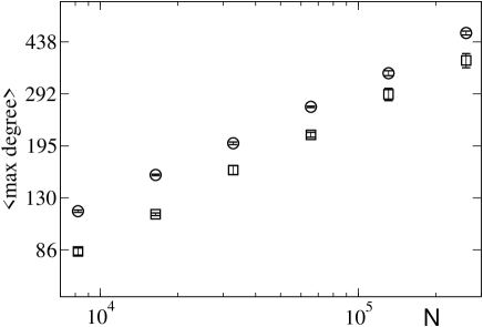
Figure 2: The evolution with $N$ of the average maximum degree of a graph for $\beta=2.1$ (circles) and $3.0$ (squares) and $N=2^{13}$ to $2^{18}$. This log-log plot illustrates the observation that for scale-free graphs with the exponent $\beta$ approaching 2, the maximum node degree evolves with $N$ at a rate close to that observed for $\beta=3$, in variance with (12). An analytic argument explaining the observed behavior is given in the text.

Our next experiment is with scale-free graphs. As in ref. bck we set kr

$$p_{n}=(\beta-1)\frac{\Gamma(2\beta-3)\Gamma(n+\beta-3)}{\Gamma(\beta-2)\Gamma(n+2\beta-3)}\propto n^{-\beta}$$ (13)

but the generated graphs are now non-degenerate with loops, instead of trees (the graphs are also, in general, not connected). Since $\langle n\rangle=2$, we also set $L=N$. We have chosen this example to illustrate a behavior which, as we shall argue in a moment, is generic. Since the same choice was made in ref. bck , the reader can directly compare the results obtained in the two ensembles studied.

The maximum node degree $n_{\mbox{\footnotesize\rm max}}$ has been measured in long runs. The results, for $\beta=2.1$ and 3.0 are shown in Fig. 2. The important point is that the rate of increase of $n_{\mbox{\footnotesize\rm max}}$ with $N$ is almost the same for the two values of $\beta$, contrary to what one can read from the r.h.s. of (12). The exponent is slightly below the value 1/2, expected asymptotically (see below). The autocorrelation time increases roughly at the same rate, from about 860 (1810) to 5460 (10300) sweeps for $\beta=2.1$ ( 3.0); in a sweep one attempts to rewire all the $L$ links of the graph. The fraction of nodes and links belonging to the giant component decreases very slowly from about 0.57 and 0.78 (0.68 and 0.81) at $N=2^{14}$ to 0.55 and 0.77 ( 0.68 and 0.81) at $N=2^{18}$.

The shape and the evolution with $N$ of the degree distribution is shown in Figs. 3 and 4. It is manifest that the distribution does approach the expected limit. However, the approach is very slow and non-uniform, especially for $\beta=2.1$ .

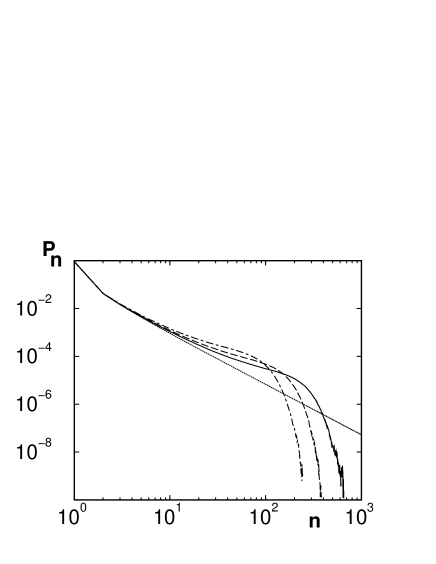
Figure 3: The degree distribution for $\beta=2.1$ and $N=2^{14}$ (dot-dashed), $2^{16}$ (dashed), $2^{18}$ (solid). The dotted line is the shape at infinite $N$. The cut-off scales like for $\beta=3$ (see the next figure). Since the distribution is normalized to unity, this results in a deviation of its shape from the asymptotic one.

Figure 4: The degree distribution for $\beta=3.0$ and $N=2^{14}$ (dot-dashed), $2^{16}$ (dashed), $2^{18}$ (solid). The dotted line is the shape at infinite $N$.

The results of the computer experiment can be understood using the following heuristic arguments:

Let $n\gg 1$ be the degree of a node in the tail, so that there is no more than one node of that degree. We consider the ensemble of degenerate graphs and we estimate the fraction of graphs where the node in question has no self- or multiple-connections. The counting is easily performed by considering the symmetric adjacency matrix $C_{ij}=\#$links $\vec{ij}$ (every undirected link contributes to two elements of $C$). Obviously, $C_{ij}$ is 0 or 1 for non-degenerate graphs, but can take any integer value for degenerate ones. Let $m$ be the label of our hub. We count the adjacency matrices satisfying $\sum_{j}C_{jm}=n$.

We take the limit $N,L\to\infty$, $L/N$ fixed and $n/N\to 0$ (notice, that it is not assumed that $n$ is kept fixed when $N$ increases, it is only less than the cut-off given by eq. (12)). In this limit, the number of degenerate graphs we are interested in is proportional to the number of ways to place $n$ elements in $N$ cells, possibly putting several elements in the same cell. The standard fomula of combinatorics does not apply because one has to take care of the contribution of the symmetry factors to graph weights. The number of graphs corrected by the appropriate weights is

$$W_{\mbox{\footnotesize\rm deg}}(n)=\sum_{\{k_{j}\}}\frac{1}{2^{k_{m}}}\prod_{j}\frac{1}{k_{j}!}\;\delta(\sum^{N}_{i=1}k_{i}-n)$$ (14)

$$=\frac{1}{2\pi}\int d\alpha e^{-in\alpha+(N-1/2)e^{i\alpha}}$$ (15)

where $k_{j}\equiv C_{jm}$. There is a self-connection when $k_{m}>0$ and a multiple connection when, for $j\neq m$, $k_{j}>1$. The symmetry factors are those mentioned at the place where we summarize the Feynman rules. We have replaced the $\delta$-function by its Fourier transform and performed the independent summations over $k_{j}$. Saddle-point integration yields

$$W_{\mbox{\footnotesize\rm deg}}(n)\propto\frac{N^{n}}{n!}$$ (16)

A similar counting of graphs where our node is neither self- nor multiply connected yields

$$W_{\mbox{\footnotesize\rm non-deg}}(n)={N-1\choose n}\propto\frac{N^{n}}{n!}\exp({-\frac{n^{2}}{2N}})$$ (17)

The ratio is foot3

$$W_{\mbox{\footnotesize\rm non-deg}}/W_{\mbox{\footnotesize\rm deg}}\propto\exp({-\frac{n^{2}}{2N}})$$ (18)

Hence, the entropy of the non-degenerate graphs is dramatically reduced compared to that of graphs with degeneracies and this reduction depends strongly on $n$. This is the origin of the bias mentioned in the preceding section:

Suppose we have generated a very large sample of scale-free graphs without any care for degeneracies. For each such graph the histogram of degrees contains a tail of sparsely located columns of unit height. However, we know, because of the mapping on the balls-in-boxes model, that the histogram for the whole sample has the shape of $p_{n}$ for $n<n_{\mbox{\footnotesize max}}$. Now, what happens when we exclude degeneracies, specifically when we check whether a node in the tail of the histogram does have the forbidden connections? Eq. (18) tells us that the rejection rate is non-uniform in $n$ and that nearly all candidate graphs will be rejected when $n$ is large compared to $N^{1/2}$.

Thus, to the exent one can neglect the fluctuations of graph weights, the degree distribution in non-degenerate graphs is expected to be cut by an additional factor, roughly behaving like $\exp{(-n^{2}/2N)}$. In the absence of dynamical correlations and for $\beta\leq 3$ the cut-off in non-degenerate graphs is expected to scale like $N^{1/2}$ and not like the r.h.s. of eq. (12), i.e. independently of $\beta\;$ ! Imposing non-degeneracy one generates, at finite $N$, parasite correlations whose manifestation is the violation of eq. (12). Notice, that this entropy argument does not apply to trees, which within the full graph ensemble have a nearly vanishing entropy and which, as shown in bck , have their own mapping on balls-in-boxes.

The conclusion of this section is that our algorithm is efficient in generating all classes of graphs for any given degree distribution. In the specific, but most interesting case, of the maximally random non-degenerate scale-free graphs whose degree distribution falls like $n^{-\beta}$, with $\beta<3$, the tail of the degree distribution is cut at $n_{\mbox{\footnotesize\rm max}}\sim N^{1/2}$. This effect prevents the finite networks from fully developing the large part of the tail of their a priori expected degree distribution. This is a feature of the model, a result of the absence of dynamical correlations, and not a failure of the algorithm foot4 .

It is known that nodes are correlated in some growing network models with a scale-free behavior kr . Here we find, independently of any specific model, that dynamical correlations seem to be needed for some networks with $\beta\approx 2$ to be observed in the real world. We also observe that the thermodynamic limit $N\to\infty$ of the maximum entropy graph model can be rather non-uniform and therefore somewhat tricky.

IV Summary and conclusion

There is much activity in producing new growing network models. Such models are invaluable for illustrating some basic dynamical mechanisms, like the preferential attachment rule ba . However, in order to understand the generic geometries of wide classes of networks it is perhaps worthwhile to adopt a complementary approach, consistently defining the corresponding statistical ensembles and working with these static ensembles using the standard tools of equilibrium statistical mechanics.

With this motivation in bck we have defined a statistical ensemble for an arbitrary node degree distribution. This ensemble is the most random possible, but clearly not the most general: we assumed that node degrees are independent, to the extent that this is possible when the number of nodes and links is fixed. In ref. bck we have rapidly focused on trees, indicating, however, that the approach extends to more complicated graphs. The discussion of the ensemble of non-degenerate graphs, those without multiple- and self-connections, has been postponed. The present paper completes ref. bck .

In particular, we have constructed here an efficient algorithm, easily implemented on a computer, which enables one to generate non-degenerate random graphs. We are ready to share our computer code with interested people, on request.

Another simple algorithm has been proposed in ref nsw ; mr and used subsequently: one first generates from a given distribution $p_{n}$ a set of node degrees $\{n_{j}\}$ and uses these numbers to construct auxiliary graphs, each with one node and $n_{j}$ half-links. In the second step one connects the half-links at random. The resulting graph is usually degenerate foot2 . Imposing the absence of degeneracies is in this approach very tedious, especially that a non-degenerate graph may just not exist for a given set $\{n_{j}\}$.

We have studied in detail the behavior of the degree distribution of finite-size graphs. In the absence of dynamical inter-node correlations, for generic scale-free non-degenerate graphs (but not trees) this distribution is cut at

$$n_{\mbox{\footnotesize\rm max}}\propto N^{\gamma}\;,\;\gamma=\min[1/2,1/(\beta-1)]$$ (19)

at asymptotically large $N$. It appears that a fat tail with $\beta$ rather close to 2 observed in some data could hardly show up if dynamical inter-node correlations were absent. And indeed, non-trivial correlations are present in models of growing networks using the preferential attachment recipe kr .

It is certainly very important to develop a theory of correlated networks. Other authors dms2 ; berg have very recently made interesting explicit proposals in that direction. Our approach can also be rather easily generalized to include dynamical correlations. This does not mean that the physics of correlated networks is transparent to us at the present time. We shall hopefully return to the problem of correlations in another publication.

Acknowledgements: We dedicate this paper to the memory of our friend and collaborator Joao D. Correia who passed away tragically last year.This work was partially supported by the EC IHP Grant HPRN-CT-1999-000161 and by Project 2 P03B 096 22 of the Polish Research Foundation (KBN) for 2002-2004. Z.B. thanks the Alexander von Humboldt Foundation for a followup fellowship. Laboratoire de Physique Théorique is Unité Mixte du CNRS UMR 8627.

References

- (1) Z. Burda, J.D. Correia, A. Krzywicki, Phys. Rev. E64, 046118 (2001).
- (2) S. Dorogovtsev, J.F.F. Mendes, A.N. Samukhin, cond-mat/0204111 .
- (3) S. Dorogovtsev, J.F.F. Mendes, A.N. Samukhin, cond-mat/0206131 .
- (4) J. Berg, M. Lässig, cond-mat/0205589
- (5) M. Bauer, D. Bernard, cond-mat/0206150
- (6) M.E.J. Newman, S.H. Strogatz, D.J. Watts, Phys. Rev. E64, 026118 (2001).
- (7) B. Bollobás, Random graphs (Academic Press, London, 1985).
- (8) A.-L. Barabási, R. Albert, Rev. Mod. Phys. 47, 74 (2002).
- (9) S.N. Dorogovtsev, J.F.F. Mendes, Adv. Phys. 51, 1079 (2002).
- (10) See any field theory textbook. A short introduction can be found in D. Bessis, C. Itzykson, J.B. Zuber, Adv. Appl. Math., 1, 109 (1980).
- (11) M. Molloy, B. Reed, Random Struct. Algorithms 6, 161 (1995); Combinatorics, Probab. Comput. 7, 295 (1998).
- (12) The factor reflects the symmetry between the two orientations of a link forming a tadpole and the factor reflects the symmetry of link permutations in an m-tuple connection between nodes.
- (13) N. Metropolis et al, J. Chem. Phys. 21, 1087 (1953); K. Binder, Monte Carlo methods in Statistical Physics (Springer, Berlin,1986); a pedagogical introduction can be found in M. Creutz, L. Jacobs, C. Rebbi, Phys. Rept. 95, 201 (1983).
- (14) P. Bialas, Z. Burda, D. Johnston, Nucl. Phys. B493 (1997) 505; Nucl. Phys. B542, 413 (1999).
- (15) Sampling links priviledges nodes with large degree. The factor eliminates the bias. One can drop this factor in the Metropolis test by selecting the link to be rewired as follows: select at random, in the register of nodes, the node . Then, pick at random one of the links converging to . With this method the mapping on the balls-in-boxes model is even more obvious, since one samples directly the nodes to be updated. In the model of ref. binb the node orders are the only degrees of freedom.
- (16) S.N. Dorogovtsev, J.F.F. Mendes, A.N. Samukhin, Phys. Rev. E63, 062101 (2001).
- (17) P.L. Krapivsky, S. Redner, Phys. Rev. E63, 066123 (2001)
- (18) Strictly speaking, the exponent on the r.h.s. is . The ratio falls faster than a Gaussian at large . The estimate given in (18) is crude. One should take into account the fact that approximately nodes have degree 1, approximately nodes have degree 2 etc. The correponding modification of the r.h.s. of (15) is straightforward, but the formulae are somewhat cumbersome. We skip this calculation, mentioning only that once it is performed, the constant 1/2 in the exponent of (18) is replaced by another constant depending on the shape of . This does not affect the scaling properties of the cut-off.
- (19) Our first guess was that, at finite , one should use a modified set of input couplings krz . We realized that it is a wrong strategy, when we undestood the entropic origin of the distorsion of the degree distribution. Another comment: It is interesting to compute the number of ”redundant” links, i.e. those producing self- and multiple connections, in the ensemble of scale-free graphs where the degeneracies have not been excluded. When the connectivity distribution has a finite support this number, in a generic graph, is expected to be small, although most graphs are degenerate. This is also the behavior we observe for . We find and at and respectively. As one moves towards 2 the situation changes dramatically. For we find respectively, for the same values of : and . This behavior can be inferred from the analytic argument of Sec. III. We do not count redundant links there, but we estimate the weight of degenerate graphs, which involves the same information.
- (20) A. Krzywicki, talk at the workshop on random geometries (Utrecht, Oct. 2001), cond-mat/0110574 .
- (21) A.-L. Barabási, R. Albert, Science 286, 509 (1999).
- (22) This construction is described in detail in ref. mr , but not as a method of constructing non-degenerate graphs, the actual object of the study of the authors. Molloy and Reed find it useful to map the ensemble of graphs they are interested in on the less constrained ensemble of ”random constructions”, i.e. degenerate graphs (this approach was earlier used by other authors, see er ). We are indebted to M. Bauer and D. Bernard for calling our attention to this point.