[

Three and four current reversals vs temperature in correlation ratchets
with a simple sawtooth potential

Abstract

Transport of Brownian particles on a simple sawtooth potential subjected to both unbiased thermal and nonequilibrium symmetric three-level Markovian noise is considered. The new effects of three and four current reversals as a function of temperature are established in such correlation ratchets. The parameter space coordinates of the fixed points associated with these current reversals and the necessary and sufficient conditions for the existence of the novel current reversals are found.

]

The aim of this paper is to study current reversals in controlled transport of Brownian particles [2] induced by symmetric nonequilibrium noise in ratchets with a simple sawtooth potential, bearing in mind potential applications for separation of nanoobjects [3]. It is known that current reversals in ratchet systems can be engendered by changing various system parameters [4, 5, 6, 7, 8, 9, 10, 11, 12, 13, 14, 15, 16], including the flatness parameter of the noise [6, 7, 8, 9, 10], the correlation time of nonequilibrium fluctuations [11], the temperature in multinoise cases [12], the power spectrum of the noise source [13], the shape of the potential [14], the number of interacting particles per unit cell [15], and the mass of the particles [16]. As a rule, these results have been obtained either at the limits of slow and fast noises or by numerical methods. At the same time, analytic results would greatly facilitate the study, especially in the intermediate regimes of the system parameters which is the realm of biology. It is especially difficult to obtain analytic expressions for the multinoise ratchets. A fortunate exception here is the symmetric three-level telegraph process (trichotomous noise) which is rich enough physically and can at the same time be treated analytically [9, 10, 17]. In this paper we will prove, on the basis of the leading order term of a series expansion for the probability current in terms of inverse flatness, that there exist three and four current reversals of the probability current as a function of temperature $D$. Never before have more than two current reversals with $D$ been reported for correlation ratchets with a simple sawtooth potential. (At the same time, in the case of rocking ratchets, infinitely many current reversals may occur [18].) We will also derive the necessary, and the necessary and sufficient conditions for the existence of these novel current reversals.

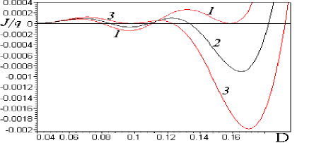
FIG. 1.: Four current reversals vs temperature $D$ for fixed $d=0.0045$ and $a=27.75$. The switching rates are respectively (1) $\nu_{1}=649.651630$, (2) $\nu_{2}=646.770000$, and (3) $\nu_{3}=643.816291$. Curve (2) has four single zeros. Curves (1) and (3) have two single zeros and one two-fold zero. (At the fixed values of $d$ and $a$, for curves with $\nu$ values smaller than $\nu_{3}$ and greater than $\nu_{1}$ there can occur at most two current reversals.)

A zero-mean trichotomous Markovian stochastic process $Z(t)$ consists of jumps between three values $z=\{a,0,-a\},\,a\!>0$. The jumps follow in time the pattern of a Poisson process, the values occuring with the stationary probabilities $P_{s}(a)=P_{s}(-a)=q$ and $P_{s}(0)=(1-2q)$, where $0\!<\!q\!<\!1/2$. Denoting the state space and the transition matrix of our trichotomous process, respectively, by $\{a_{i}\}\!:=\!\{a,\,0,-a\}$ and $T_{ij}:=P\{a_{i},t+\!\tau\,|a_{j},t\}$, $\;i,j=1,2,3,\;\tau>0$, we have

$$\Big{(}T_{ij}\Big{)}=\Big{(}\delta_{ij}\Big{)}+\pmatrix{q-1&q&q\cr 1-2q&-2q&1-2q\cr q&q&q-1\cr}\big{(}1-e^{-\nu\tau}\big{)},$$ (1)

where $\nu\!>\!0$. In a stationary state, the fluctuation process satisfies $\langle{Z(t)}\rangle=0$ and $\langle{Z(t+\tau)Z(t)}\rangle=2qa^{2}\exp(-\nu\tau)$, where the switching rate $\nu$ is the reciprocal of the noise correlation time $\tau_{c}=1/\nu$, i.e. $Z(t)$ is a symmetric zero-mean exponentially correlated noise. The trichotomous process is a particular case of the kangaroo process [6] with flatness parameter $\varphi:=\langle{Z^{4}(t)}\rangle/\langle{Z^{2}(t)}\rangle^{2}=1/(2q)$.

At great flatness, $q\to 0$, which is the case addressed in the present paper, the transition matrix of our trichotomous process takes the following form

$$\Big{(}T_{ij}\Big{)}=\Big{(}\delta_{ij}\Big{)}+\pmatrix{-1&0&0\cr 1&0&1\cr 0&0&-1\cr}\big{(}1-e^{-\nu\tau}\big{)}+{\cal O}(q).$$ (2)

Within the framework of the three-level noise models used in Refs. [7, 8] flatness is determined by a parameter $\lambda$, which regulates the relative amount of time spent in the state $z=0$ as opposed to the states $z=a$ and $z=-a.\;$ If $\lambda\to 0$, the flatness $\varphi\to\infty$ and the leading order terms in the transitions matrixes of the noise processes of Refs. [7, 8] and Eq. (2) become equivalent. Thus, at great flatness our trichotomous noise practically coincides with the noise used by Bier [7] and Elston-Doering [8].

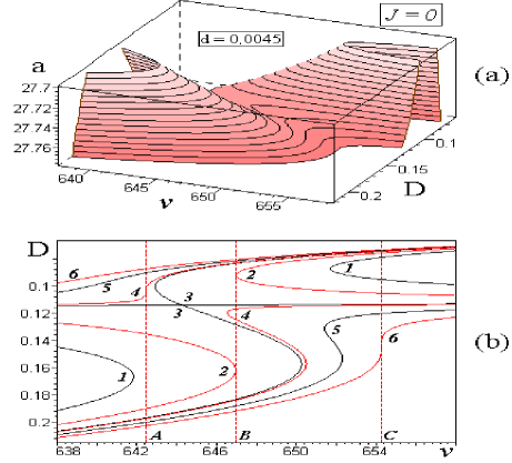
FIG. 2.: (a) The surface of current reversals $J(D,a,\nu)=0$ for a fixed asymmetry parameter $d=0.0045$. (b) The projection of the surface onto plane $(D,\nu)$. The level curves correspond to the following values of the noise amplitude: (1) $a=27.700000$, (2) $a=27.733329$, (3) $a=27.753662$, (4) $a=27.755045$, (5) $a=27.765482$, (6) $a=27.775920.$ The effect begins at $\nu_{A}=642.4480$ and ends at $\nu_{C}=654.2591$; whereas at $\nu_{B}=646.9504$ there occur two two-fold zeros.

We describe overdamped motion of Brownian particles in dimensionless units by the Langevin equation

$${dX\over dt}=h(X)+\xi(t)+Z(t),\quad h(x)\equiv-{dV(x)\over dx},$$ (3)

where $V(x)=V(x+1)$ is a periodic spatial potential of period 1. The thermal noise satisfies $\langle\xi(t)\rangle=0$ and $\langle\xi(t_{1})\xi(t_{2})\rangle$ $=2D\delta(t_{1}-t_{2})$, where $D$ is the thermal noise strength which will below simply be called the temperature, for the sake of brevity. As said, we take the random force $Z(t)$ to be a zero-mean trichotomous Markovian stochastic process [9, 10, 17]. To derive an exact formula for $J$, the Fokker-Planck master equation corresponding to Eq. (3) is used, supposing that the potential $V(x)$ in Eq. (3) is piecewise linear (sawtooth-like) and its asymmetry is determined by a parameter $d\in(0,1)$, with $d=1/2$ for symmetric $V(x)$. The force caused by the potential is $h(x)=b:=1/d$ for $x\in(0,d)$ and $h(x)=-c:=-1/(1-d)$ for $x\in(d,1)$. Under these assumptions, a complex exact formula as a quotient of two eleventh-order determinants can be derived for the probability current $J$. To obtain a more manageable formula, on the assumption that the flatness parameter is large, $\varphi=1/(2q)\gg 1$, we can expand the current in a series $J=qJ^{(1)}+q^{2}J^{(2)}+\ldots\;$ One of the present authors derived for the leading order term $qJ^{(1)}$ a rather lengthy analytic expression, i.e., Eqs. (31)-(33) in Ref. [10]. Herein we shall apply graphical analysis to study the analytic expression of $qJ^{(1)}$ in the intermediate regimes.

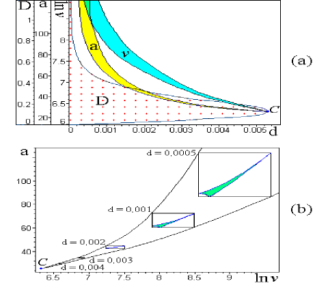
FIG. 3.: (a) The necessary and (b) the necessary and sufficient conditions for the four-current-reversal effect. The dotted region in (a) displays the possible range of the four zeros of the current $J(D)$ at different values of $d$.

First we will briefly review the asymptotic limits of the current $J$ as the function of $\nu$ and $D$, found in Ref. [10]. In the case of large flatness at the asymptotic limits of both small and large $\nu$ the function $J=J(\nu)$ is always positive. Hence, in the case under discussion there can exist either none or an even number of current reversals with $\nu$. Two current reversals vs $\nu$ (as well as $D$) were addressed by Ref. [10]. The case of four current reversals vs $\nu$ with the necessary and sufficient conditions for their existence was extensively discussed in our earlier paper [19].

What concerns current reversals as functions of $D$, then in the asymptotic limit of high temperature, $D\to\infty$, we find that

$$J\approx{q(b-c)a^{2}\over 180bcD^{4}}.$$ (4)

Thus, at high temperatures the behavior of the function $J=J(D)$ is uniform: the current is always positive and decreases monotonically to zero as $D\to\infty$. At low temperatures, in the cases $a<c$ and $c<a<b$ the current is positive for all values of $\nu$ and $d$. For $a>b$ the current behaves asymptotically as

$$J\approx q\nu\left\{\left[e^{\nu/c(a-c)}-e^{-\nu/b(a+b)}\right]^{-1}\right.-$$ (5)

$$-\left.\left[e^{\nu/b(a-b)}-e^{-\nu/c(a+c)}\right]^{-1}\right\}.$$ (6)

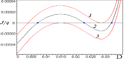
FIG. 4.: Three current reversals vs temperature $D$ for fixed $d=0.005$ and $a=255.86$. Switching rates are (1) $\nu_{1}=3.17379365$, (2) $\nu_{2}=3.17381112$, and (3) $\nu_{3}=3.17382860$. Curve (2) has three single zeros. Curves (1) and (3) have one single and one two-fold zero.

Notably, $J$ is positive in the case of $a\leq bc$ at any $\nu$. If $a>bc$, then the current reverses to negative at a critical value $\nu=\nu_{0}$. The point of reversal $\nu_{0}$, being a nontrivial solution of the transcendental equation $J(\nu_{0})=0$, can be found by numerical calculation from Eq. (6). In the limit of low temperatures, $D\to 0$, the behavior of the function $J=J(D)$ is not uniform. Depending on the values of the remaining parameters of the system, at $D=0$ the function $J=J(D)$ may have a (finite) positive, a (finite) negative or a zero value and may start to increase, decrease or remain practically constant for a while as the temperature $D$ increases [10]. What is important about the asymptotic limits in the context of the present paper, where we are interested in the behavior of the current in the intermediate domains of the system parameters, is the fact that at the limit of large $D$ the function $J=J(D)$ is always positive, whereas at the limit of small $D$ it can be either negative or positive, and, consequently, there can occur any number, odd or even, of current reversals with $D$.

Before the present paper not more than two current reversals with respect to $D$ had been found for correlation ratchets with a simple sawtooth potential. Moreover, in a paper [10] by one of the authors it was even argued that the possible number of current reversals with temperature is either zero, one, or two.

Next we will examine the four-current-reversal effect as a function of $D$ (see Fig. 1). Fig. 2(b) exhibits the level curves of zero current, $J(D,\nu;d,a)=0$, for fixed $d=0.0045$ at different fixed values of $a=\text{const}$. The level curves may be considered as functions $\nu=\nu(D)$ (as well as $D=D(\nu)$), with $d$ and $a$ being parameters. In Fig. 2(b) the level curves on the left close at smaller finite values of $\nu$ (not shown), whereas both branches of the level curves on the right approach zero as $\nu$ grows. Regarding the upper branch on the right, if $a<d^{-1}(1-d)^{-1}$, then $D$ becomes zero only at the limit $\nu\to\infty$, whereas if $a>d^{-1}(1-d)^{-1}$, then $D$ is zero at a finite $\nu$. In view of this, two types of the level curves are distinguishable in Fig. 2(b): namely, the connected ones (i.e., curves (4)-(6)) and the ones (i.e., curves (1) and (2) comprising two components, viz., a closed curve and a curve with one end open. There is one very special level curve (i.e., curve (3)) which intersects itself at the saddle point. The four current reversals vs $D$ effect exists at a certain fixed value of $\nu_{\rm{fixed}}=\text{const}$ if and only if there exist $d$ and $a$ for which the function $\nu=\nu(D;d,a)$ has a local maximum $\nu_{\text{max}}>\nu_{\rm{fixed}}$ and a local minimum $\nu_{\text{min}}<\nu_{\rm{fixed}}$ (see the vertical dashed lines in Fig. 2(b)).

By gradually varying $a$ and $d$ one can demonstrate that the region of existence of the four-current-reversal effect as a function of $D$ shrinks to a $4$-point $C$, which has the following coordinates: $d_{C}\approx 0.0053305,a_{C}\approx 25.3379050,D_{C}\approx 0.1244425$ and $\ln\nu_{C}\approx 6.2977305$. The four-current-reversal effect is possible if $d\in(0,d_{C}),a\in(a_{C},\infty)$ and $\nu\in(\nu_{C},\infty)$ (see Fig. 3). The necessary conditions for the existence of the four-current-reversal effect are shown in Fig. 3(a) by the shaded regions in planes $(d,a)$ and $(d,\nu)$, and in Fig. 3(b) by the region between the ascending outermost curves in plane $(\nu,a)$, while the intensively shadowed narrow wedge-shaped areas in Fig. 3(b) fix the values of $d,a,$ and $\nu$, which are necessary and sufficient for the existence of the four-current-reversal effect as a function of $D$.

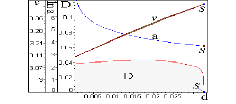
FIG. 5.: The necessary conditions for the three-currentreversal vs $D$ effect. The curves $a=a(d)$ and $\nu=\nu(d)$ represent actually narrow regions in the planes $(d,a)$ and $(d,\nu)$. Especially narrow is the bow depicted by $a=a(d)$, e.g., at $d=0.001$ the noise ranges from $a_{\rm{min}}=1280.330$ to $a_{\rm{max}}=1280.462$.

What concerns the three-current-reversal effect as a function of temperature $D$ (see Fig. 4), then the effect occurs only in a very narrow range of the system parameters $a$ and $\nu$ (see Fig. 5). By varying $a$ and $d$ step by step, we will see that the region of existence of the three-current-reversal effect as a function of $D$ shrinks to a critical $4$-point $S$ in the parameter space, which has the following coordinates: $d_{S}\approx 0.03275$, $D_{S}=0$, $a_{S}\approx 38.95953$, $\nu_{S}\approx 3.42833$. The three-current-reversal effect is possible if $d\in(0,d_{S})$, $\nu\in(3.1275,\nu_{S})$ and $a\in(a_{S},\infty)$ (see Fig. 5).

As demonstrated above, the necessary and sufficient conditions for the existence of an odd number of current reversals vs $D$ are $a>bc$ and $\nu>\nu_{0}$, where $\nu_{0}$ is a zero of the function $J(\nu)$, see Eq. (6). In the opposite case, the number of current reversals is even or zero. To elucidate the physical meaning of the above conditions, let us re-derive Eq. (6) on the grounds of the following physical considerations. In the case of great flatness, $q\ll 1$, the noise $Z(t)$ is with overwhelming probability, $P_{s}(0)=1-2q\approx 1$, at the state $z=0$ and the current $J$ can be regarded as the sum $J=J^{+}+J^{-}$, where the positive current $J^{+}$ is caused by the transitions $z\!=\!a\leftrightarrow z\!=\!0$ and the negative current $J^{-}$ by the transitions $z\!=\!-a\leftrightarrow z\!=\!0$. (Note that the transitions $z\!=\!a\leftrightarrow z\!=\!-a$ induce current which is proportional to $q^{2}$ and will be discarded at the present approximation.) Under these assumptions the stationary probability distribution at the noise state $z=0$ with $D=0$ consists, evidently, of delta functions at $x=\pm n+d,\;n=0,1,2,\dots\;$ Within the interval $(0,1)$ the center of mass lies at $y_{0}=d$. Let at the initial moment occur the transition $z\!=\!0\rightarrow z\!=\!-a$. The first time when the noise turns back to $z=0$ is denoted by $t_{0}$. The center of mass stabilizes now at the position $y$. It is easy to find that the center of mass is shifted by $\Delta y(t_{0})=y-y_{0}$ with $\Delta y(t_{0})=-(n+1)$ if $(n+1)T^{-}>t_{0}\geq nT^{-}+T_{1}^{-}$ and $\Delta y(t_{0})=-n$ if $nT^{-}+T_{1}^{-}>t_{0}\geq nT^{-}$. The interval $T^{-}=T_{1}^{-}+((1-d)/(a+c))$ is the time that the particle for $z=-a$ takes to pass the period $L=1$ of the potential; $T_{1}^{-}=d/(a-b)$ is the time necessary for passing the length $d$ (i.e., from the minimum of the potential to the maximum in the negative direction). The probability $W(t_{0})$ that in a certain time interval $(0,t_{0})$ the transitions $z\!=\!-a\rightarrow z\!=\!0$ do not occur, is given by $W(t_{0})=\exp\,(-\nu t_{0})$. The probability that such a transition will occur within the time interval $(t_{0},t_{0}+dt_{0})$ is $\nu dt_{0}$, and consequently, $<\Delta y>=\nu\int_{0}^{\infty}e^{-\nu t_{0}}\Delta y(t_{0})dt_{0}$. Considering that the average number of transitions per unit time into the $z\!=\!-a_{0}$ state is $q\nu$, we obtain $J^{-}\!=q\nu<\Delta y>\,=\!-q\nu W(T_{1}^{-})/[1-W(T^{-})]$. Similarly, one can derive the positive component of the current, viz. $J^{+}\!=q\nu W(T_{1}^{+})/[1-W(T^{+})]$, where $T_{1}^{+}\!=(1-d)/(a-c)$, $T^{+}\!=T_{1}^{+}\!+d/(a+b)$. The inequality $T^{+}\!<T^{-}$ being equivalent to $d<1/2$ , it is evident that the total current $J=J^{+}\!+J^{-}$, whose expression coincides exactly with Eq. (6), can be negative only when $T_{1}^{-}\!<T_{1}^{+}$. The latter inequality can be written as $a>bc$, which is just the necessary condition.

Following similar trains of thought as above in the case of low temperature $D\ll 1$ and replacing the passage times $T^{\pm}$ and $T_{1}^{\pm}$ by respective mean first passage times $<T^{\pm}>$ and $<T_{1}^{\pm}>$, one can re-derive the necessary conditions for the existence of the three-current-reversal effect as a function of temperature. Namely, we obtain the formulas $a=41/(32d)\!-\!0.25$ and $\nu_{0}\!=3.12(1\!+3d)$ which quite well approximate the corresponding curves in Fig. 5.

Finally we will discuss the possible usefulness of the phenomena of three and four current reversals. One of the first applications of the Brownian ratchet mechanism has been to separate particles by size, charge, mass, etc. Separation can be achieved even if there are no current reversals, as particles of different viscous friction move at different speeds. If there is only one current reversal, then particles of different friction coefficients. move in the opposite directions within the same environment. If there occur two current reversals with $\nu$, then particles with parameter values within a characteristic interval can be separated, as they move in the direction opposite to that of the remaining particles. However, it is known that the two zeros of the current $J(\nu)$ generally occur at largely displaced values of $\nu$. Therefore, in the opposite direction move those particles whose friction coefficients are within a wide interval and the separation effect is of low selectivity. Though this wide interval can be made narrower by varying the other system parameters, the really narrow intervals occur only in the vicinity of the transition regimes (i.e., the transition from two current reversals to zero current reversals), where the absolute value of the current is small. On the other hand, the three-current-reversal with $D$ effect enables us to design continuous two-step separation schemes with very high selectivity within a narrow $\nu$ interval. Note that at a fixed value of $d$ the range of values of $\nu$ where the three-current-reversal vs $D$ effect exists is very narrow indeed (see Fig. 5).

Within the framework of the calculation scheme of the present paper, the absolute value of the net current is inversely proportional to the flatness parameter of the trichotomous noise, $\varphi=1/(2q)$, and $q$ as an expansion parameter is generally considered to be infinitesimal. However, we have managed to show by direct numerical calculations without using expansion in $q$ that the effects are present up to $q\approx 0.015$.

Beyond the separation methods, the phenomena of three and four current reversals may be of interest in biology, e.g., when considering the motion of macromolecules. While it is known that the two-current-reversal effect allows one pair of motor-proteins to move simultaneously in opposite directions along the microtubulae inside the eucariotic cells, then existence of three and four current reversals will enable such a simultaneous motion of many pairs of motor proteins. Whether the intracellular transport makes use of the flashing ratchet mechanism as one presently tends to think, or the correlation ratchets mechanism, or a combination of them remains to be seen.

To summerize, it is remarkable that the interplay of the symmetric three-level and thermal noises in the ratchets with a simple sawtooth potential generates such a rich variety of cooperation effects as up to four current reversals with temperature as well as switching rate. The results are the more surprising because in analogous model systems with the symmetric dichotomous noise the current reversals are altogether absent.

We acknowledge partial support by the Estonian Science Foundation Grants Nos 4042 and 4208.

REFERENCES

- [1] E-mail address: tammelo@ut.ee
- [2] P. Reimann, Phys. Rep. 361, 57, (2002).
- [3] A. Ajdari and J. Prost, C.R. Acad. Sci. Paris II 315, 1635 (1992); J. Rousselet, L. Salome, A. Ajdari, and J. Prost, Nature 370, 446 (1994); S. Leibler, ibid. 370, 412 (1994); M. Bier and R.D. Astumian, Phys. Rev. Lett. 76, 4277 (1996); G.W. Slater, H.L. Guo, and G.I. Nixon, Phys. Rev. Lett. 78, 1170 (1997); C. Kettner, P. Reimann, P. Hänggi, and F. Müller, Phys. Rev. E 61, 312 (2000).
- [4] A. Mielke, Ann. Physik (Leipzig) 4, 476 (1995).
- [5] T. Hondou and Y. Sawada, Phys. Rev. E 54, 3149 (1996).
- [6] C.R. Doering, W. Horsthemke, and J. Riordan, Phys. Rev. Lett. 72, 2984 (1994).
- [7] M. Bier, Phys. Lett. A 211, 12 (1996).
- [8] T.C. Elston and C.R. Doering, J. Stat. Phys. 83, 359 (1996).
- [9] R. Mankin, A. Ainsaar, and E. Reiter, Phys. Rev. E 61, 6359 (2000)
- [10] R. Mankin, A. Ainsaar, A. Haljas, and E. Reiter, Phys. Rev. E 63, 041110 (2001).
- [11] R. Bartussek, P. Hänggi, B. Lindner, and L. Schimansky-Geier, Physica D 109, 17 (1997); C. Berghaus, U. Kahlert, and J. Schnakenberg, Phys. Lett. A 224, 243 (1997).
- [12] J. Kula, T. Czernik, and J. Łuczka, Phys. Rev. Lett. 80, 1377 (1998).
- [13] M.M. Millonas and M.I. Dykman, Phys. Lett. A 185, 65 (1994).
- [14] P. Reimann and T.C. Elston, Phys. Rev. Lett. 77, 5328 (1996); M. Kostur and J. Łuczka, Phys. Rev. E 63, 021101 (2001).
- [15] I. Derényi and A. Ajdari, Phys. Rev. E 54, R5 (1996).
- [16] F. Marchesoni, Phys. Lett. A 237, 126 (1998).
- [17] R. Mankin, A. Ainsaar, and E. Reiter, Phys. Rev. E 60, 1374 (1999).
- [18] P. Jung, J.G. Kissner, and P. Hänggi, Phys. Rev. Lett. 76, 3436 (1996); D. Dan, M.C. Mahato, and A.M. Jayannavar, Phys. Rev. E 63, 056307 (2001).
- [19] R. Mankin, R. Tammelo, and D. Martila, Phys. Rev. E 64, 051114 (2001).