[

$SU(4)$ Fermi Liquid State and Spin Filtering in a Double Quantum Dot System

Abstract

We study a symmetrical double quantum dot (DD) system with strong capacitive inter-dot coupling using renormalization group methods. The dots are attached to separate leads, and there can be a weak tunneling between them. In the regime where there is a single electron on the DD the low-energy behavior is characterized by an $SU(4)$-symmetric Fermi liquid theory with entangled spin and charge Kondo correlations and a phase shift $\pi/4$. Application of an external magnetic field gives rise to a large magneto-conductance and a crossover to a purely charge Kondo state in the charge sector with $SU(2)$ symmetry. In a four lead setup we find perfectly spin polarized transmission.

]

Introduction.— Quantum dots are one of the most basic building blocks of mesoscopic circuits[1]. In many respects quantum dots act as large complex atoms coupled to conducting leads that are used to study transport. The physical properties of these dots depend essentially on the level spacing and precise form of the coupling to the leads: They can exhibit Coulomb blockade phenomena [2], build up correlated Kondo-like states of various kinds[3, 4, 5], or develop conductance fluctuations.

The simplest mesoscopic circuits that go beyond single dot devices in their complexity are double dot (DD) devices (see Fig. 1). These ’artificial molecules’ have been extensively studied both theoretically [6, 7, 8, 9, 10, 11] and experimentally [12, 13, 14, 15]: They may give rise to stochastic Coulomb blockade[6] and peak splitting[7, 12], can be used as single electron pumps[1], were proposed to measure high frequency quantum noise[11], and are building blocks for more complicated mesoscopic devices such as turn-stiles or cellular automata [16]. DD’s also have interesting degeneracy points where quantum fluctuations may lead to unusual strongly correlated states[17].

In the present paper we focus our attention to small semiconducting DDs with large inter-dot capacitance [10, 17]. We consider the regime where the gate voltages $V_{\pm}$ are such that the lowest lying charging states, $(n_{+},n_{-})=(0,1)$ and $(1,0)$, are almost degenerate: $E(1,0)-E(0,1)\approx 0$ [$n_{\pm}=$ $\#$ of extra electrons on dot ’$\pm$’, and $E(n_{+},n_{-})$ is measured from the common chemical potential of the two leads]. We consider the simplest, most common case where the states $(1,0)$ and $(0,1)$ have both spin $S=1/2$, associated with the extra electron on the dots. Then at energies below the charging energy of the DD, ${\tilde{E}}_{C}\equiv\min\{E(1,1)-E(0,1),E(0,0)-E(0,1)\}$, the dynamics of the DD is restricted to the subspace $\{S^{z}=\pm 1/2;\;n_{+}-n_{-}=\pm 1\}$.

As we discuss below, quantum fluctuations between these four quantum states of the DD generate an unusual strongly correlated Fermi liquid state, where the spin and charge degrees of freedom of the DD are totally entangled. We show that this state possesses an $SU(4)$ symmetry corresponding to the total internal degrees of freedom of the DD, and is characterized by a phase shift $\delta=\pi/4$. This phase shift can be measured by integrating the DD device in an Aharonov-Bohm interferometer[18]. Application of an external field on the DD suppresses spin fluctuations. However, charge fluctuations are unaffected by the magnetic field and still give rise to a Kondo effect in the charge (orbital) sector [10, 17, 19]. We show that in a four lead setup this latter state gives rise to an almost totally spin polarized current through the DD with a field-independent conductance $G\approx e^{2}/h$. The conductance across the dots, on the other hand, shows a large negative magneto-resistance at $T=0$ temperature.

Model.— Let us first discuss the arrangement in Fig. 1. At energies below ${\tilde{E}}_{C}$ we describe the isolated DD in terms of the orbital pseudospin $T^{z}\equiv{(n_{+}-n_{-})/2}=\pm\frac{1}{2}$:

$$H_{\rm dot}=-\delta E\;\;T^{z}-t\;T^{x}-B\;S^{z}\;.$$ (1)

The term proportional to $T^{z}$ describes the energy difference of the two charge states [$\delta E\equiv E(1,0)-E(0,1)\sim V_{+}-V_{-}$ for a fully symmetrical system], while $t\ll{\tilde{E}}_{C}$ is the tunneling amplitude between them. The last term stands for the Zeeman-splitting due to an applied local magnetic field in the $z$ direction. We are interested in the regime, where — despite the large capacitive coupling,— the tunneling between the dots is small. Furthermore, one needs a large enough single particle level spacing $\Delta$ on the dots. Both conditions can be satisfied by making small dots [20], which are close together or capacitively coupled to a common top-gate electrode [21].

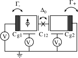
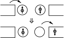
FIG. 1.: Top: Schematics of the DD device. Bottom: Virtual process leading to ’spin-flip assisted tunneling’ as described in Eq. (4)

The leads are described by the Hamiltonian:

$$H_{\rm leads}=\sum_{|\varepsilon|<D}\epsilon\;a^{\dagger}_{\varepsilon\sigma+}a_{\varepsilon\sigma+}+\sum_{|\varepsilon|<D}\epsilon\;a^{\dagger}_{\varepsilon\sigma-}a_{\varepsilon\sigma-}\;,$$ (2)

where $a^{\dagger}_{\varepsilon\sigma+}$ ($a^{\dagger}_{\varepsilon\sigma-}$) creates an electron in the right (left) lead with energy $\varepsilon$ and spin $\sigma$, $D\sim{\rm min}\{{\tilde{E}}_{C},\Delta\}\equiv 1$ is a cut-off, and $\{a^{\dagger}_{\varepsilon\sigma\tau},a_{\varepsilon^{\prime}\sigma^{\prime}\tau^{\prime}}\}=\delta_{\tau\tau^{\prime}}\delta_{\sigma\sigma^{\prime}}\delta(\varepsilon-\varepsilon^{\prime})$.

To determine the effective DD – lead coupling we have to consider virtual charge fluctuations to the excited states with $n_{+}+n_{-}=0$ and 2, generated by tunneling from the leads to the dots. By second order perturbation theory in the lead-dot tunneling we obtain the following effective Hamiltonian:

$$H_{\rm Kondo}={1\over 2}J_{+}P_{+}{\vec{S}}(\psi^{\dagger}{\vec{\sigma}}\;p_{+}\psi)+{1\over 2}J_{-}P_{-}{\vec{S}}(\psi^{\dagger}{\vec{\sigma}}\;p_{-}\psi),$$ (3)

$$H_{\rm assist}=Q_{\perp}\left[T^{+}{\vec{S}}(\psi^{\dagger}{\vec{\sigma}}\tau^{-}\psi)\;\;+\;\;\mbox{h.c.}\right],$$ (4)

$$H_{\rm orb}={1\over 2}\Big{(}V_{z}T^{z}(\psi^{\dagger}\tau^{z}\psi)+V_{\perp}[T^{+}(\psi^{\dagger}\tau^{-}\psi)+\mbox{h.c.}]\Big{)}.$$ (5)

where $\psi_{\sigma\tau}=\int d\varepsilon\;a_{\varepsilon\sigma\tau}$, and ${\vec{\sigma}}$ and ${\vec{\tau}}$ denote the spin and orbital pseudospin of the electrons ($\sigma=\uparrow,\downarrow$; $\tau=\tau^{z}=\pm 1$). The operators $P_{\pm}=(1\pm 2T^{z})/2$ and $p_{\pm}=(1\pm\tau^{z})/2$ project out the DD states $(1,0)$ and $(0,1)$, and the right/left lead channels, respectively.

In the limit of small dot-lead tunneling the dimensionless exchange couplings are $J_{\pm}\sim\Gamma_{\pm}/{\tilde{E}}_{C}$ with $\Gamma_{\pm}$ the tunneling rate to the right (left) lead [22]. The ’spin-flip assisted tunneling’ $Q_{\perp}\sim\sqrt{\Gamma_{+}\Gamma_{-}}/{\tilde{E}}_{C}$ in Eq. (4) gives simultaneous spin- and pseudospin-flip scattering and is produced by virtual processes depicted in the lower part of Fig. 1, while the spin-independent parts of such virtual processes lead to the orbital Kondo term in Eq. (5) with similar amplitudes.

We first focus on the case of a fully symmetrical DD. Then the sum of Eqs. (3) and (4) can be rewritten as:

$$H_{\rm Kondo}+H_{\rm assist}={1\over 2}{J}{\vec{S}}(\psi^{\dagger}{\vec{\sigma}}\psi)\;$$ (6)

$$+ {Q_{z}}T^{z}{\vec{S}}(\psi^{\dagger}\tau^{z}{\vec{\sigma}}\psi)+{Q_{\perp}}\left(T^{+}{\vec{S}}(\psi^{\dagger}\tau^{-}{\vec{\sigma}}\psi)+\mbox{h.c.}\right)\;,$$ (7)

where $J=Q_{z}=(J_{+}+J_{-})/4$. The couplings in Eqs. (3-5) are not entirely independent, but are related by the constraints $V_{\perp}=Q_{\perp}$ and $J=Q_{z}$.

Scaling Analysis.— The perturbative scaling analysis follows that of a related model in Ref. [23]. In the perturbative RG one performs the scaling by integrating out conduction electrons with energy larger than a scale scale $\tilde{D}\ll D$, and thus obtains an effective Hamiltonian that describes the physics at energies $\tilde{D}$. For $\delta E=t=B=0$, in the leading logarithmic approximation we find that all couplings diverge at the Kondo temperature $T_{K}^{(0)}$, where the perturbative scaling breaks down. Nevertheless, the structure of the divergent couplings suggests that at low energies $J=V_{\perp}=V_{z}=Q_{\perp}=Q_{z}$. Thus at small energies, — apart from a trivial potential scattering — the effective model is a remarkably simple SU(4) symmetrical exchange model:

$$H_{\rm eff}(T\to 0)=\tilde{J}\sum_{\alpha,\beta=1,..,4}\psi_{\alpha}^{\dagger}\psi_{\beta}\;|\beta\rangle\langle\alpha|\;,$$ (8)

where the index $\alpha$ labels the four combinations of possible spin and pseudospin indices, and the $|\alpha\rangle$’s denote the four states of the DD. This indeed can be more rigorously proven using strong coupling expansion, conformal field theory, and large $f$ (flavor) expansion techniques [24, 25, 26], and is also confirmed by our numerical computations.

Numerical Renormalization Group (NRG).— To access the low-energy physics of the DD, we used Wilson’s NRG approach[27]. In this method one defines a series of rescaled Hamiltonians, $H_{N}$, related by the relation [27]:

$${H}_{N+1} \equiv \Lambda^{1/2}{H}_{N}+\sum_{\sigma\tau}\xi_{N}\left(f^{\dagger}_{N,\sigma\tau}f_{N+1,\sigma\tau}+\mbox{h.c}\right),$$ (9)

where $f_{0\sigma\tau}=\psi_{\sigma\tau}/\sqrt{2}$ and $H_{0}\equiv 2\Lambda^{1/2}/(1+\Lambda)\;H_{\rm int}$ with $\Lambda\sim 3$ as discretization parameter, and $\xi_{N}\approx 1$. (For the definition of $f_{N}$ see Ref. [27].) We have defined $H_{\rm int}=H_{\rm dot}+H_{\rm Kondo}+H_{\rm assist}+H_{\rm orb}$. The original Hamiltonian is related to the $H_{N}$’s as $H=\lim_{N\to\infty}\omega_{N}H_{N}$ with $\omega_{N}=\Lambda^{-(N+1)/2}(1+\Lambda)/2$. Solving Eq. (9) iteratively we can then use the eigenstates of $H_{N}$ to calculate physical quantities at a scale $T,\omega\sim\omega_{N}$.

Results.— First let us consider the case $H_{\rm dot}=0$.

Fixed point structure.— The finite size spectrum produced by the NRG procedure contains a lot of information. Among others, we can identify the structure of the low-energy effective Hamiltonian from it [27], and also determine all scattering phase shifts.

In particular, we find that for $\delta E=t=B=0$ the entire finite size spectrum can be understood as a sum of four independent, spinless chiral fermion spectra with phase shifts $\delta=\pi/4$. This phase shift is characteristic for the $SU(4)$ Hamiltonian, Eq. (8), and simply follows from the Friedel sum rule [24]. Application of an external magnetic field $B$ to the DD gradually shifts $\delta$ to the values $\delta_{\uparrow}\to\pi/2$ and $\delta_{\downarrow}\to 0$ [28].

Spectral functions.— To learn more about the dynamics of the DD we computed at $T=0$ the spin spectral function $\varrho_{S}^{z}(\omega)=-(1/\pi){\rm Im}\{\chi_{S}^{z}(\omega)\}$, and pseudospin spectral function $\varrho_{\tau}^{y}(\omega)=-(1/\pi){\rm Im}\{\chi_{\tau}^{y}(\omega)\}$ by the density matrix NRG method [29].

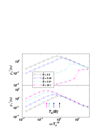
FIG. 2.: $T=0$ spin and pseudospin spectral functions for $J=Q_{z}=V_{z}=0.14$, $V_{\perp}=Q_{\perp}=0.13$, and various values of $\tilde{B}\equiv B/T_{K}^{(0)}$. For $B=0$ both the spin and pseudospin spectral functions exhibit $\sim\omega$ behavior below the Kondo temperature $T^{(0)}_{K}\sim 10^{-3}$. Applying a magnetic field the situation changes: The $B>T^{(0)}_{K}$ magnetic field destroys the spin Kondo correlations and leads to a purely orbital Kondo-effect.

At $B=0$ the various spectral functions exhibit a peak at the same energy, $T^{(0)}_{K}$, corresponding to the formation of the $SU(4)$ symmetric state (see Fig. 2). Below $T^{(0)}_{K}$ all spectral functions become linear, characteristic to a Fermi liquid state with local spin and pseudospin susceptibilities $\chi_{S}\sim\chi_{T}\sim 1/T^{(0)}_{K}$, where the $SU(4)$ ”hyper-spin” of the dot electron (formed by $\{\uparrow+,\downarrow+,\uparrow-,\downarrow-\}$ components) is screened by the lead electrons.

Now let us consider the case $H_{\rm dot}\neq 0$. In a large magnetic field, $T^{(0)}_{K}\ll B$, spin-flip processes are suppressed: The spin spectral function therefore shows only a Schottky anomaly at $\omega\sim B$. Nevertheless, the couplings $V_{\perp}$ and $V_{z}$ still generate a purely orbital Kondo state in the spin channel with the same orientation as the DD spin, with a reduced Kondo temperature $T_{K}(B)<T^{(0)}_{K}$, and a corresponding phase shift $\delta_{\uparrow}=\pi/2$.

Due to the spin-pseudospin symmetric structure of the Hamiltonian, Eq. (6), the opposite effect occurs for a large $\delta E$: In that limit the charge is localized on one side of the DD, charge fluctuations are suppressed, and the system scales to a spin Kondo problem. A large tunneling, $t>T_{K}^{(0)}$ is also expected to lead to a somewhat similar effect, though the conductance through the DD behaves very differently in the two cases [28].

DC Conductivity.— First we focus on the conductivity across the DD assuming a small tunneling $t$. Then we can assume that the two dots are in equilibrium with the leads connected to them, and we can compute the induced current perturbatively in $t$. A simple calculation yields the following formula:[30]

$$G={{2\pi^{2}e^{2}}\over h}\;\;{t^{2}}\;\;\lim_{\omega\to 0}{\varrho_{\tau}^{y}(\omega)\over\omega}\;.$$ (10)

The normalized DC conductance at $T=0$ temperature is shown in Fig 3. Below the orbital Kondo temperature $\varrho_{\tau}^{y}(\omega)\sim\omega/T^{2}_{K}(B)$, leading to a dimensionless conductance $\sim[t/T_{K}(B)]^{2}$. However, $T_{K}(B)$ strongly decreases with increasing $B$ implying a large negative magneto-resistance in the $T=0$ DC conductance. This effect is related to the correlation between spin and orbital degrees of freedom. We have to emphasize that the simple considerations above only apply in the regime $t\ll T_{K}(B)$. For larger values of $t$ a more complete calculation is needed.

Having extracted the phase shifts from the NRG spectra, we can construct the scattering matrix in more general geometries too and compute the $T=0$ conductance using the Landauer-Buttiker formula [28, 31, 32]. In the perfectly symmetrical two terminal four lead setup of Fig. 4 with $\delta E=t=0$, e.g., the DC conductance is $G_{13}={1\over 2}G_{Q}(\sin^{2}(\delta_{\downarrow}(B))+\sin^{2}(\delta_{\uparrow}(B)))$, where $G_{Q}=2e^{2}/h$ is the quantum conductance. By the Friedel sum rule $\delta_{\uparrow}(B)=\pi/2-\delta_{\downarrow}(B)$, and thus $G_{13}(T=0)=G_{Q}/2$, independently of $B$. However, the polarization of the transmitted current, $P=2\sin^{2}(\delta_{\uparrow})-1$ tends rapidly to 1 as $B>T_{K}^{(0)}$, and the DD thereby acts as a perfect spin filter at $T=0$ with $B>T_{K}^{(0)}$, and could also serve as a spin pump. For a typical $T_{K}\approx 0.5K$ and a $g$-factor $g\approx-0.4$ as in GaAs, e.g. a field of $2.5T$ would give a $97\%$ polarized current. This efficiency is comparable to other spin filter designs [33]. By lowering $T_{K}$, much higher polarizations could be obtained.

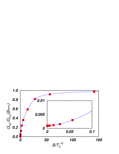
FIG. 3.: The $T=0$ conductance of DD system at $\omega=0$ for $J=Q_{z}=0.14$, $V_{\perp}=Q_{\perp}=0.13$, $V_{z}=0.14$ and different magnetic field values. Inset: small $B$ limit of the conductance.

Robustness.— Since the spin $S^{\alpha}$ and pseudospin $T^{\alpha}$ are both marginal operators at the $SU(4)$ fixed point [25], we conclude that the $SU(4)$ behavior is stable in the sense that a small but finite value of $\delta E$, $B$, $t\ll T_{K}^{(0)}$ will lead only to small changes in physical properties like the phase shifts. The anisotropy of the couplings is also irrelevant in the RG sense [25, 26], and the role of $J_{-}\neq J_{+}$ symmetry breaking is only to renormalize the bare value of $\delta E$, which is a marginal perturbation itself. Therefore the $SU(4)$ Fermi liquid state is robust under the conditions discussed in the Introduction.

Experimental accessibility.— For our scenario it is crucial to have large enough charging energy and level spacing ${\tilde{E}}_{C},\Delta>T_{K}^{(0)}>t$. With today’s technology it is possible to reach $\Delta\sim 2-3{\rm K}$. The dot-dot capacitance (and thus ${\tilde{E}}_{C}$ [7]) can be increased by changing the shape of the gate electrode separating the dots, using a columnar geometry as in Refs. [19, 34], where the two-dimensional dots are placed on the top of each other, or placing an additional electrode on the top of the DD device[21]. We could not find a closed expression for $T_{K}^{(0)}$ in the general case. However, for a symmetrical DD $J\approx V_{\perp}\approx V_{z}\approx Q_{\perp}\approx Q_{z}\sim\Gamma/2\pi{\tilde{E}}_{C}$, provided that fluctuations to the $(0,0)$ state give the dominant contribution. Then we obtain $T_{K}^{(0)}\approx De^{-1/4J}$ and $T_{K}(B=\infty)\approx{\rm cst.}\;{[T_{K}^{(0)}]}^{2}/D$. Thus the value of $J$ and thus $T_{K}^{(0)}$ can be tuned experimentally to a value similar to the single dot experiments. Indeed, an orbital Kondo effect has recently been observed [19].

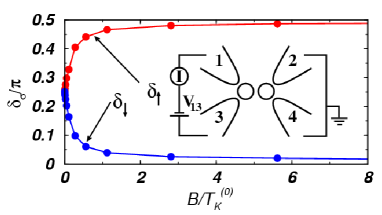
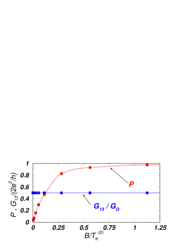
FIG. 4.: Top: Magnetic field dependence of the phase shifts for $t=\delta E\approx 0$. Bottom: Corresponding $T=0$ dimensionless conductance and spin polarization of the current in the four lead setup shown in the Top inset.

Summary.— We have studied a DD system with large capacitive coupling close to its degeneracy point, in the Kondo regime. Using both scaling arguments and a non–perturbative NRG analysis, we showed that the simultaneous appearance of the Kondo effect in the spin and charge sectors results in an $SU(4)$ Fermi liquid ground state with a phase shift $\pi/4$. Upon applying an external magnetic field, the system crosses over to a purely charge Kondo state with a lower $T_{K}$. In a four–terminal setup, the DD could thus be used as a spin filter with high transmittance. We further predict a large serial magneto-conductance at $T=0$. The $SU(4)$ behavior in this system is robust, and is experimentally accessible.

Acknowledgements: We are grateful to T. Costi, K. Damle, and D. Goldhaber-Gordon for discussions. This research has been supported by NSF Grants Nos. DMR-9981283 and Hungarian Grants No. OTKA F030041, T038162, and N31769. W.H. acknowledges financial support from the German Science Foundation (DFG).

REFERENCES

- [1] L.P. Kouwenhoven et al. in Mesoscopic Electron Transport, eds. L.L. Sohn et al., NATO ASI Series E, vol. 345, pp. 105-214 (Kluwer, Dordrecht, 1997).
- [2] R. Wilkins et al., Phys. Rev. Lett. 63, 801 (1989).
- [3] D. Goldhaber-Gordon et al., Nature 391, 156 (1998); S.M. Cronenwett et al., Science 281, 540 (1998).
- [4] W.G. van der Wiel et al., Phys. Rev. Lett. 88, 126803 (2002).
- [5] L.I. Glazman and K.A. Matveev, Sov. Phys. JETP 71, 1031 (1990).
- [6] I.M. Ruzin et al., Phys. Rev. B 45, 13469 (1992).
- [7] J. M. Golden and B. I. Halperin, Phys. Rev. B 53, 3893 (1996).
- [8] K.A. Matveev et al., Phys. Rev. B 54, 5637 (1996).
- [9] W. Izumida and O. Sakai, Phys. Rev. B 62, 10260 (2000).
- [10] T. Pohjola et al., Europhys. Lett. 55, 241 (2001).
- [11] R. Aguado and L.P. Kouwenhoven, Phys. Rev. Lett. 84, 1986 (2000).
- [12] F.R. Waugh et al., Phys. Rev. Lett. 75, 705 (1995).
- [13] L.W. Molenkamp et al., Phys. Rev. Lett. 75, 4282 (1995).
- [14] R.H. Blick et al., Phys. Rev. B 53, 7899 (1996).
- [15] T.H. Oosterkamp et al., Phys. Rev. Lett. 80, 4951 (1998).
- [16] G. Tóth et al., Phys. Rev. B 60, 16906 (1999).
- [17] D. Boese et al., Phys. Rev. B 64, 125309 (2001).
- [18] A. Yacoby et al., Phys. Rev. Lett. 74, 4047 (1995).
- [19] U. Wilhelm et al., Physica E. 14, 385 (2002)
- [20] D. Goldhaber-Gordon (private communication).
- [21] I.H. Chan et al., Appl. Phys. Lett. 80, 1818 (2002).
- [22] The energy dependence of couplings generates irrelevant terms in the RG sense and can therefore be neglected.
- [23] G. Zaránd, Phys. Rev. B 52, 13459 (1995).
- [24] P. Nozières and A. Blandin, J. Phys. 41, 193 (1980).
- [25] J. Ye, Phys. Rev. B 56, R489 (1997).
- [26] G. Zaránd , Phys. Rev. Lett. 76, 2133 (1996).
- [27] K.G. Wilson, Rev. Mod. Phys. 47, 773 (1975); T. Costi, in Density Matrix Renormalization, edited by I. Peschel et al. (Springer 1999).
- [28] L. Borda et al. (unpublished).
- [29] W. Hofstetter, Phys. Rev. Lett. 85, 1508 (2000).
- [30] This formula can also be used at .
- [31] M. Pustilnik and L. I. Glazman, Phys. Rev. Lett. 85, 2993 (2000).
- [32] R. Landauer, IBM J. Res. Dev. 1, 223 (1957); D.S. Fisher and P.A. Lee, Phys. Rev. B 23, 6851 (1981); M. Büttiker, Phys. Rev. Lett. 57, 1761 (1986).
- [33] R. M. Potok et al., preprint cond-mat/0206379.
- [34] M. Pi, et al., Phys. Rev. Lett. 87, 066801 (2001).