Casimir Forces: An Exact Approach for Periodically Deformed Objects

Abstract

A novel approach for calculating Casimir forces between periodically deformed objects is developed. This approach allows, for the first time, a rigorous non-perturbative treatment of the Casimir effect for disconnected objects beyond Casimir’s original two-plate configuration. The approach takes into account the collective nature of fluctuation induced forces, going beyond the commonly used pairwise summation of two-body van der Waals forces. As an application of the method, we exactly calculate the Casimir force due to scalar field fluctuations between a flat and a rectangular corrugated plate. In the latter case, the force is found to be always attractive.

Casimir forces between electrically neutral solids are a macroscopic consequence of material dependent changes in the zero-point vacuum fluctuations of the electromagnetic field Casimir48 ; Milonni+Mostepanenko-book ; Bordag-review . The Casimir effect for two parallel metallic plates has been referred to as one of the least intuitive consequences of quantum electrodynamics Schwinger+78 . However, this effect can be as well regarded as a macroscopic manifestation of many-body van der Waals forces between the particles that form the plates. This point of view is supported by Schwinger’s approach which considers no vacuum fluctuations but only the fields generated by the fluctuating dipoles themselves Schwinger+78 . In addition, fluctuation induced forces can be observed in a plethora of other systems where quantum-, thermal or disorder fluctuations are modified by external objects Kardar+99 . Examples of recent interest are as diverse as the thickening of Helium films near the superfluid transition Israelachvili-book ; Garcia+02 , forces between vortex matter in anisotropic superconductors Buechler+00/Mukherji+97 , Casimir energy densities in cosmological models Bytsenko+96 , and interactions between proteins on biological membranes Israelachvili-book .

Initiated by the first quantitative verification of the electrodynamic Casimir effect by Lamoreaux Lamoreaux97 , high precision experiments have motivated a resurgence in the field of Casimir force measurements in the last few years Mohideen+Chan+Bressi . All experiments confirm the theory for Casimir’s original flat plate geometry within a few percent of accuracy. Much less clear is the situation for non-trivial geometries. If the separation between the objects is large compared to characteristic wavelengths of the material, e.g., the plasma wavelength, the force becomes a universal function of the geometry with the energy scale set by $\hbar$. However, the entropic origin and collective nature of the Casimir force can cause this universal function to have a non-trivial and unexpected dependence on the shape of the interacting objects. There is little intuition even as to whether the interaction is attractive or repulsive as demonstrated strikingly by the positivity of the Casimir energy of a conducting spherical shell Boyer74 . In particular, the latter result raises the important question if repulsive forces can also emerge between disconnected objects, being of potential importance for the behavior of microelectromechanical systems due to the short-scale separations between their mobile parts Serry+95 . Recently, non-trivial shape dependencies have been probed experimentally by tailoring the shape of the plates in Casimir’s geometry Roy+99 ; Chen+02 .

Calculations of Casimir forces beyond the simple situation of two parallel flat plates are notoriously difficult due to the collective nature of the many-body interaction. To date, this simple geometry indeed appears to be the only case amongst disconnected macroscopic objects for which an exact result is available. This is due to the lack of rigorous, non-perturbative methods for calculating the force between deformed objects. The simplest and commonly used approximation is the pairwise summation (PWS) of van der Waals forces Bordag-review . However, Lifshitz’s theory for dielectric bodies (with flat surfaces) demonstrates that in general the interaction cannot be obtained from such an approximation Lifshitz56 . In view of the fact that the PWS approximation can even give the wrong sign for the Casimir interaction, e.g., for a conducting cubic shell Barton01 , it is fair to conclude that this approach is to some extent uncontrolled. For corrugated metal plates, the failure of PWS for small corrugation lengths has been shown by perturbation theory with respect to the deformation amplitude Emig+01 . Another perturbative approach is based on a multiple scattering expansion but has been applied only in the limit of large separations between the objects Balian+78 . However, with regard to potential sign changes in the interaction and experimentally realized separations, it is highly desirable to gather information about the perturbatively non-accessible regime where the distance between the objects is of the same order as the deformation amplitude.

In this Letter we will introduce an avenue along which the shortcomings of the commonly used approximations can be bypassed for objects with uniaxial shape modulations. To illustrate our new approach, we consider the force between a rectangular corrugated and a flat plate, a geometry which cannot be treated by perturbation theory due to the edges in the surface profile. Before coming to this specific case, let us outline the general approach. In uniaxial geometries the electromagnetic field and thus also the Casimir force can be represented as a sum of transversal magnetic (TM) and electric (TE) wave contributions Emig+01 . In order to simplify the analysis, we will consider here only TM waves, which are governed by the scalar field Euclidean action

$$S[\Phi]=\frac{1}{2}\int d^{4}X(\nabla\Phi)^{2}$$ (1)

after a Wick rotation to imaginary time. For TM waves we have to impose Dirichlet boundary conditions, $\Phi_{|S}=0$ on the surfaces $S$. TE waves can be treated analogously by imposing Neumann boundary conditions with suppressed normal gradient of $\Phi$. The geometry consists of a flat surface in the $xy$-plane at $z=H$ and a uniaxially corrugated surface given by $z=h(x)$ with periodic height profile $h(x+\lambda)=h(x)$ of wavelength $\lambda$. At zero temperature, the Casimir force per surface area $F=-\partial{\cal E}/\partial H$ between the two objects corresponds to the change with the objects distance in the ground state energy density ${\cal E}$ of the field $\Phi$. This zero temperature theory is applicable as long as the de Broglie wavelength of photons, $\lambda_{T}=\hbar c/k_{B}T$, is much larger than the mean separation between the objects.

Employing the path integral method to implement the boundary conditions at the surfaces Li+91 ; Golestanian+97 , the energy density is given by ${\cal E}=-\hbar c\ln{\cal Z}/AL$ with $L$ the Euclidean system size along imaginary time and

$${\cal Z}={\cal Z}_{0}^{-1}\int{\cal D}\Phi\prod_{\bf r}\delta[\Phi({\bf r},h(x))]\delta[\Phi({\bf r},H)]e^{-S[\Phi]/\hbar},$$ (2)

with the partition function ${\cal Z}_{0}$ of empty space with no objects, and ${\bf r}=(ict,x,y)\equiv(X_{0},X_{1},X_{2})$. The delta functions can be rewritten as a functional integral over an auxiliary field on each surface so that after integrating out $\Phi$, the new action is quadratic with matrix kernel

$$M({\bf r},{\bf r}^{\prime})=\left(\!\!\begin{array}[]{cc}G[{\bf r}-{\bf r}^{\prime},h(x)\!-\!h(x^{\prime})]&G[{\bf r}-{\bf r}^{\prime},H\!-\!h(x^{\prime})]\\ G[{\bf r}-{\bf r}^{\prime},H\!-\!h(x)]&G[{\bf r}-{\bf r}^{\prime},0]\end{array}\!\!\right)$$ (3)

and Green’s function $G({\bf r},z)=({\bf r}^{2}+z^{2})^{-1}/4\pi^{2}$ Hanke+02 . The Casimir force per surface area $A$ between the objects is then given by

$$F=-\frac{\hbar c}{2AL}\partial_{H}\ln\det M=-\frac{\hbar c}{2AL}{\rm Tr}\left(M^{-1}\partial_{H}M\right).$$ (4)

This expression is suited for a non-perturbative approach since the force must be finite, in contrast to the energy density ${\cal E}$ which contains without an explicit cutoff also infinite but $H$ independent contributions from the individual surfaces.

In the more conventional approaches, the zero-point energy is calculated in terms of the allowed frequencies $\omega_{n}$ of the space between the objects, using ${\cal E}=\frac{1}{2}\sum_{n}\hbar\omega_{n}$ and by applying subtraction schemes in order to obtain a regularized energy which in turn yields the force. An advantage of our approach is that the frequencies need not to be calculated explicitly but the force is directly obtained in terms of the free space Green’s function without any necessity for regularization schemes. Of course, the functional inverse of the matrix kernel $M({\bf r},{\bf r}^{\prime})$ in Eq. (4) is in general difficult to evaluate. In the following, we will demonstrate how this problem can be tackled for uniaxial geometries. Due to the symmetry of the geometry, it is useful to consider the matrix kernel $M({\bf p},{\bf q})$ in momentum space. The periodicity of the surface profile along the $X_{1}$ direction and uniformity in the $X_{0}X_{2}$ plane impose the general form

$$M({\bf p},{\bf q}) = \sum_{m=-\infty}^{\infty}N_{m}(p_{\perp},p_{1})\,(2\pi)^{3}\,\delta({\bf p}_{\perp}+{\bf q}_{\perp})$$ (5)

$$\times\,\delta(p_{1}+q_{1}+2\pi m/\lambda)$$

on the kernel. This Fourier decomposition defines the matrices $N_{m}(p_{\perp},p_{1})$ with ${\bf p}_{\perp}=(p_{0},p_{2})$ and $p_{\perp}=|{\bf p}_{\perp}|$. Thus the matrix $M({\bf p},{\bf q})$ has non-vanishing entries only along the diagonal and its periodically shifted analogues. An important observation is that matrices of this structure can be transformed to block-diagonal form by applying row and column permutations. Physically, the existence of such a transformation is due to the non-mixing property of the kernel $M({\bf p},{\bf q})$ for Fourier modes whose moments differ by non-integer multiples of $2\pi/\lambda$. For the time being, let us assume that the objects have the extension $W$ along the $X_{1}$ direction, leading to a discrete set of momenta $p_{1}$. Then the transformed matrix $M({\bf p},{\bf q})$ consists of block matrices $M_{j}$ along the diagonal with $j=1,\ldots,N=W/\lambda-1$. Since this matrix form can be always realized by an even number of permutations, we get

$$\det M={\prod}_{j=1}^{N}\det M_{j}.$$ (6)

The block matrices $M_{j}$ can be expressed in terms of the matrices $N_{m}$ of the decomposition in Eq. (5). For discrete momenta in $x$ direction, the matrices $M_{j}$ can be parametrized by integer indices $k$, $l=-\infty,\ldots,\infty$, leading to the result

$$M_{j,kl}({\bf p}_{\perp},{\bf q}_{\perp})=(2\pi)^{2}\delta({\bf p}_{\perp}+{\bf q}_{\perp})B_{kl}(p_{\perp},2\pi j/W)$$ (7)

with the matrix $B_{kl}$ given by

$$B_{kl}(p_{\perp},p_{1})=N_{k-l}(p_{\perp},p_{1}+2\pi l/\lambda).$$ (8)

Moreover, from Eq. (6) we obtain easily $\partial_{H}(\ln\det M)=\sum_{j=1}^{N}{\rm Tr}(M_{j}^{-1}\partial_{H}M_{j})$. Thus the separation dependent part of the ground state energy ${\cal E}$ is given by the sum of the individual energies of the decoupled subsystems which are described by the matrices $M_{j}$. Next, it is useful to define the function

$$g(p_{\perp},p_{1})={\rm tr}\left(B^{-1}(p_{\perp},p_{1})\partial_{H}B(p_{\perp},p_{1})\right),$$ (9)

where the lower case symbol tr denotes the partial trace with respect to the discrete indices $k$, $l$, cf. Eq. (8), at fixed $p_{\perp}$, $p_{1}$. It follows from the structure of the matrix $B_{kl}$ that $g(p_{\perp},p_{1}+2\pi n/\lambda)=g(p_{\perp},p_{1})$. In addition, choosing the height profile to be symmetric, $h(-x)=h(x)$, imposes the condition $N_{m}(p_{\perp},-p_{1})=N_{-m}(p_{\perp},p_{1})$ on the matrices $N_{m}$ which in turn leads after row and column permutations of the matrix $B_{kl}$ to $g(p_{\perp},-p_{1})=g(p_{\perp},p_{1})$. Taking at this point the thermodynamic limit $W$, $N\to\infty$, transforms the sum over the energies of the $N$ subsystems into an integral. Thus we obtain, after taking the total trace over all degrees of freedom, the final result for the Casimir force density,

$$F=-\frac{\hbar c}{4\pi^{2}}\int_{0}^{\infty}dp_{\perp}p_{\perp}\int_{0}^{\pi/\lambda}dp_{1}\,g(p_{\perp},p_{1}),$$ (10)

where we have used the symmetries of $g(p_{\perp},p_{1})$. For a given Fourier decomposition of the kernel $M$ into the matrices $N_{m}$, this formula together with Eqs. (8), (9) yields the exact result for the force between the objects. This result has the advantage of being particularly suited for a numerical analysis as will be shown below.

In the following, we apply the general formula in Eq. (10) to obtain a non-perturbative result for the force between a flat and a rectangular corrugated surface. We choose the height profile on a basic interval as $h(x)=a$ for $|x|<\lambda/4$ and $h(x)=-a$ for $\lambda/4<|x|<\lambda/2$ so that $H$ is the mean distance between the surfaces, see Fig. 1.

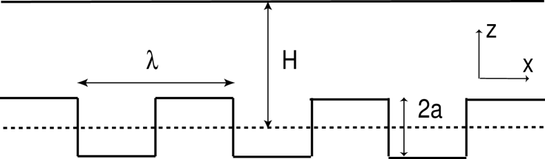
Figure 1: Cross section along the $xz$-plane of the two-plate configuration with translational invariance in $y$ direction.

This profile allows for an analytical decomposition of the kernel into matrices $N_{m}(p_{\perp},p_{1})$; details of the calculation will be published elsewhere. The result is

$$N_{0} = \left(\begin{array}[]{cc}\frac{1}{2p}+\frac{e^{-2ap}-1}{4p}+\Phi_{0}({\bf p})&\frac{e^{-pH}}{2p}\cosh(ap)\\ \frac{e^{-pH}}{2p}\cosh(ap)&\frac{1}{2p}\end{array}\right),$$ (13)

$$N_{m} = c_{m}\left(\begin{array}[]{cc}0&\frac{e^{-pH}}{2p}\sinh(ap)\\ \frac{e^{-\tilde{p}_{m}H}}{2\tilde{p}_{m}}\sinh(a\tilde{p}_{m})&0\end{array}\right),$$ (16)

for odd $m\neq 0$, and

$$N_{m}=\left(\begin{array}[]{cc}\Phi_{m}({\bf p})&0\\ 0&0\end{array}\right),$$ (17)

for even $m\neq 0$ with $\tilde{p}_{m}=\sqrt{p_{\perp}^{2}+(p_{1}+2\pi m/\lambda)^{2}}$, $c_{m}=2(-1)^{(|m|-1)/2}/\pi|m|$ and

$$\Phi_{m}({\bf p})=\frac{(-1)^{m/2}}{\pi^{2}}\!\sum_{n=-\infty}^{\infty}\!\frac{f[p_{\perp},p_{1}+(2n-1)2\pi/\lambda]}{(2n-1)(m-2n+1)},$$

where $f(p_{\perp},p_{1})=(\exp(-2ap)-1)/p$. In order to calculate the function $g(p_{\perp},p_{1})$, we truncate the matrix $B_{kl}$ symmetrically around $(k,l)=(0,0)$ at order $M$ so that $k$, $l=-(M-1)/2,\ldots,(M-1)/2$. This defines via Eq. (9) a series of approximations $g_{M}(p_{\perp},p_{1})$ which converges to $g(p_{\perp},p_{1})$ for $M\to\infty$.

Before using the general form of the decomposition, let us consider two instructive limiting cases. In the limit $\lambda/a\to 0$, one would expect that $g_{M}(p_{\perp},p_{1})$ converges very rapidly since the contributions from matrices $N_{m}$ decrease with $m$, cf. Eq. (5). To test this guess, we make use of the fact that the matrices $N_{m}(p_{\perp},p_{1}+2\pi l/\lambda)$ simplify considerably for $\lambda/a\to 0$ so that the series $g_{M}$ can be explicitly obtained order by order from the truncated matrix $B_{kl}$. Using Eq. (9), we get

$$g_{M}(p_{\perp},p_{1})=\left\{\begin{array}[]{cc}-\frac{2p(1+e^{-2ap})}{1+e^{-2ap}-2e^{2(H-a)p}}&\mbox{\rm for $M=1$}\\ -\frac{2p}{1-e^{2p(H-a)}}&\mbox{\rm for $M\geq 3$}\end{array}\right.$$ (18)

for positive $a$. This result indeed shows a rather rapid convergence; the series $g_{M}$ is even invariant for $M\geq 3$ with increasing dimension of the matrix $B_{kl}$. Using Eq. (10), we get the force density

$$F_{0}=-\frac{\pi^{2}}{480}\frac{\hbar c}{(H-a)^{4}}.$$ (19)

Physically, this result appears to be quite natural since the most contributing modes of the fluctuating field cannot probe the valleys of the corrugated surface in the limit $\lambda/a\to 0$. Thus, the surfaces experience a force which is given by the force between two flat surfaces at reduced distance $H-a$, corresponding to Eq. (19) Emig+01 . In the following we call this limit the reduced distance (RD) regime. For small $a/H$, the correction $\sim\hbar c|a|/H^{5}$ to the flat surface result is non-analytic in $a$, and thus cannot be obtained in perturbation theory.

Next, we consider the limit $\lambda/H\to\infty$. In the limit of small surface curvature, the pairwise summation (PWS) of renormalized van der Waals forces is justified Derjaguin34 . For a general surface profile, such a summation corresponds to a spatial average over $x$ of the Casimir energy for two flat surfaces, taken at the local distance $H-h(x)$ Chen+02 . For the geometry of Fig. 1, this procedure obviously yields

$$F_{\infty}=-\frac{\pi^{2}}{480}\frac{\hbar c}{2}\left(\frac{1}{(H+a)^{4}}+\frac{1}{(H-a)^{4}}\right)$$ (20)

since 50% of the local surface’s distances are $H+a$, $H-a$, each.

In order to see how the previously discussed limits fit into the complete theory as described by Eq. (10), one has to resort to a numerical analysis. The recipe for this analysis is straightforward: At fixed order $M$, the truncated matrix $B_{kl}$ is calculated from Eqs. (17), then its inverse is constructed to obtain the $M^{\rm th}$ order approximation $g_{M}$ to the function $g$. Finally, numerical integration in Eq. (10) yields a corresponding series of force densities which can be extrapolated to the final result for $M\to\infty$. The results are summarized in Figures 2 and 3. For fixed $\lambda/a$, the relative increase $\delta=F/F_{\rm flat}-1$ of the force compared to the force between two flat surfaces is shown in Fig. 2. At small $\lambda/a$ the exact result $F_{0}$ of Eq. (19) is recovered. For larger $\lambda/a$ there is a crossover between two scaling regimes: For $H\gg\lambda$ the RD scaling $\delta\sim H^{-1}$ remains valid with an amplitude which decreases with increasing $\lambda/a$. For $H\ll\lambda$ the PWS regime is entered with $\delta\sim H^{-2}$. As a consequence, the force is always attractive with $F_{0}$ as upper and $F_{\infty}$ as lower bound. Fig. 3 shows the crossover between the PWS and the RD regimes for fixed separations $H/a$. Independent of $H/a$, the crossover appears at $\lambda/a\approx 10$. The two limits are approached as $(F_{0}-F)/F_{\rm flat}\sim\lambda/a$ for $\lambda\to 0$ and $(F-F_{\infty})/F_{\rm flat}\sim a/\lambda$ for $\lambda\to\infty$, cf. the inset of Fig. 3.

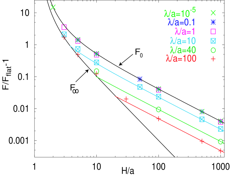
Figure 2: Relative increase of the Casimir force density $F$ for the geometry of Fig. 1 compared to the result $F_{\rm flat}=-\pi^{2}/480\times\hbar c/H^{4}$ for two flat surfaces.

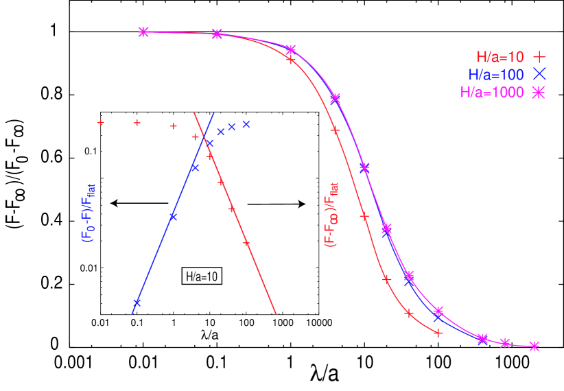
Figure 3: Crossover between the PWS ($F\to F_{\infty}$) and the RD ($F\to F_{0}$) regimes for fixed $H/a$. Inset: Scaling behavior of $F$ for the approach to $F_{0}$ for $\lambda\to 0$ and to $F_{\infty}$ for $\lambda\to\infty$.

The reported results may stimulate new developments in a large class of systems with fluctuation induced interactions. Most intriguing might be the possibility of a repulsive force for the full electromagnetic field due to anomalous contributions from the TE modes Emig+01 . Further extensions may include many-body interactions for more than two objects and the dynamic Casimir effect.

- (1)
- (2) H. B. G. Casimir, Proc. K. Ned. Akad. Wet. 51, 793 (1948).
- (3) P. W. Milonni, The Quantum Vacuum (Academic, San Diego, 1994); V. M. Mostepanenko and N. N. Trunov, The Casimir effect and its Applications (Clarendon, Oxford, 1997).
- (4) M. Bordag, U. Mohideen, and V. M. Mostepanenko, Phys. Rep. 353, 1 (2001).
- (5) J. Schwinger, L. L. DeRaad, Jr., and K. A. Milton, Ann. Phys. 115, 1 (1978).
- (6) M. Kardar and R. Golestanian, Rev. Mod. Phys. 71, 1233 (1999).
- (7) J. Israelachvili, Intermolecular and Surface Forces (Academic Press, San Diego, 1992).
- (8) R. Garcia and M. H. W. Chan, Phys. Rev. Lett. 88, 086101 (2002).
- (9) H. P. Büchler, H. G. Katzgraber, G. Blatter, Physica C 332, 402 (2000); S. Mukherji and T. Nattermann, Phys. Rev. Lett. 79, 139 (1997).
- (10) A. A. Bytsenko, G. Cognola, L. Vanzo, S. Zerbini, Phys. Rep. 266, 1 (1996).
- (11) S. K. Lamoreaux, Phys. Rev. Lett. 78, 5 (1997).
- (12) U. Mohideen and A. Roy, Phys. Rev. Lett. 81, 4549 (1998); H. B. Chan et al., Science 291, 1941 (2001); Phys. Rev. Lett. 87, 211801 (2001); G. Bressi et al., Phys. Rev. Lett. 88, 041804 (2002).
- (13) T. Boyer, Phys. Rev. A 9, 2078 (1974).
- (14) F. M. Serry, D. Walliser, and G. J. Maclay, J. Microelectromech. Syst. 4, 193 (1995).
- (15) A. Roy and U. Mohideen, Phys. Rev. Lett. 82, 4380 (1999).
- (16) F. Chen, U. Mohideen, G. L. Klimchitskaya, and V. M. Mostepanenko, Phys. Rev. Lett. 88, 101801 (2002).
- (17) E. M. Lifshitz, Sov. Phys. JETP 2, 73 (1956).
- (18) G. Barton, J. Phys. A 34, 4083 (2001).
- (19) T. Emig, A. Hanke, R. Golestanian, and M. Kardar, Phys. Rev. Lett. 87, 260402 (2001).
- (20) R. Balian and B. Duplantier, Ann. Phys. (N.Y.) 112, 165 (1978).
- (21) H. Li and M. Kardar, Phys. Rev. Lett. 67, 3275 (1991); Phys. Rev. A 46, 6490 (1992).
- (22) R. Golestanian and M. Kardar, Phys. Rev. Lett. 78, 3421 (1997); Phys. Rev. A 58, 1713 (1998).
- (23) In general, the kernel is multiplied by the metric functions of the surfaces. However, these factors can be ignored here since they drop out in the result for the force; we are indebted to A. Hanke for calling attention to this fact in the context of correlation functions, cf. A. Hanke and M. Kardar, Phys. Rev. E 65, 046121 (2002).
- (24) B. Derjaguin, Kolloid Z. 69, 155 (1934).