Collapse or Swelling Dynamics of Homopolymer Rings:
Self-consistent Hartree approach

Abstract

We investigate by the use of the Martin - Siggia - Rose generating functional technique and the self - consistent Hartree approximation, the dynamics of the ring homopolymer collapse (swelling) following an instantaneous change into a poor (good) solvent conditions.The equation of motion for the time dependent monomer - to - monomer correlation function is systematically derived. It is argued that for describing of the coarse - graining process (which neglects the capillary instability and the coalescence of “pearls”) the Rouse mode representation is very helpful, so that the resulting equations of motion can be simply solved numerically. In the case of the collapse this solution is analyzed in the framework of the hierarchically crumpled fractal picture, with crumples of successively growing scale along the chain. The presented numerical results are in line with the corresponding simple scaling argumentation which in particular shows that the characteristic collapse time of a segment of length $g$ scales as $t^{*}\sim\zeta_{0}g/\tau$ (where $\zeta_{0}$ is a bare friction coefficient and $\tau$ is a depth of quench). In contrast to the collapse the globule swelling can be seen (in the case that topological effects are neglected) as a homogeneous expansion of the globule interior. The swelling of each Rouse mode as well as gyration radius $R_{g}$ is discussed.

I Introduction

The equilibrium theory of the coil - globule transition is one of the major issues in polymer physics. Many theories have been developed to understand this physical phenomena in more detail. Gennes ; Gennes1 ; Grosberg ; Kremer . The theory for kinetics of this transition abrams01 ; Gennes2 ; Pitard ; Pitard1 ; Pitard2 ; Brochard ; Halperin ; Klushin ; Byrne ; Timoshenko ; Shakh ; Chang as well as the pertinent experiment Wu is the subject which has recently attracted a broad interest. One of the main motivations for these studies is that the first stage of a protein folding process is believed to be a fast collapse to a compact but nonspecific state. This has been shown for example by lattice Monte Carlo simulations Socci . The first stage of folding appears as sequence - independent and therefore the process is similar to the collapse of a homopolymer. Generally the collapse of a polymer chain can be addressed to an (abrupt) change of the second virial coefficient from the good solvent regime $v>0$ to the poor solvent regime $v<0$. The second virial coefficient depends on the temperature and has a Boyle point $v=0$ at the so called $\theta$ temperature. The resulting attractive two body interactions requires at least the third virial (always positive) which prevents the chain from the collapse to a single point.

In de Gennes’ “expanding sausage model” Gennes2 a flexible chain changes its conformations on a shortest scale through the formation of crumples after being quenched to poor solvent conditions. Then crumples are formed on a larger scale, resulting in a sausage - like shape, which eventually leads to a compact globule. One can see that this model is translational invariant along the chain backbone, provided that the chain has cyclic boundary conditions. This simplifies the problem and allows us later on the use of simple Rouse transformations Pitard ; Pitard1 ; Doi of the chain coordinates.

Concerning de Gennes’ model, it is shown by Brownian dynamics simulations Byrne , that the “sausages” becomes unstable with respect to capillary waves. Consequently a so called pearl necklace structure is formed. This brought about a number of publications where scaling arguments Brochard ; Halperin ; Klushin and the Gaussian self - consistent approach Timoshenko have been put forward. Actually the pearl necklace formation breaks the translational invariance along the chain backbone and complicates these issues.

Alternative recent phenomenological considerations are put forward by joining scaling argument abrams01 and computer simulations abrams01 ; Chang . It was argued abrams01 that the relaxations times related with the capillary instability as well as with coalescence of pearls are short compared to the characteristic time on which the “sausage” change its configuration. Since the positions of pearls along the chain are random they can be averaged over. The resulting “sausage” can be seen as an envelop (which has the form of a flexible cylinder) of the pearl necklaces and the overall chain configurations are composed by random walks of sausages. This picture successfully explains the so called coarse - graining process shortly after the quench to a range of temperature below $\theta$ - point, but above eventual glassy globular relaxation regimes Pitard2 ; Dokholyan ; Rost . This argumentation reconciles in a sense the two scenarios mentioned above, but the microscopic picture is still lacking. Therefore instead of considering the processes of formation and coalescence of pearls we concentrate here on the coarse - grained dynamics of the “sausage”. This model, as it was already mentioned, is homogeneous in the sense that the translational invariance along the chain backbone is effectively assured during the process of the collapse.

In this paper we provide the microscopic theory for the coil to globule transition. In order to get insight and some intuitive picture for the later discussion we start from the scaling consideration. Then we study the Langevin dynamics of the problem based on the Martin - Siggia - Rose (MSR) generating functional technique together with the self - consistent Hartree approximation Horner ; Shapir ; Rost1 . It is quite important for the judgment of the final results how the low molecular solvent dynamics is treated. In this paper we restrict our consideration to the random phase approximation (RPA) which is well - known in the context of the theory of both polymeric Vilgis and low - molecular Boon systems. The RPA fails to account the hydrodynamic interaction because in the hydrodynamic regime collisions dominate and keep the solvent in a state of local thermodynamic equilibrium (see e.g. Sec.6.5 in ref. Boon ), so that we leave this subject for the future publications. As a main result the generalized dynamical equation for the collapsed (or swelled) chain has been derived. The relaxation laws for the early and late stages are investigated analytically, whereas the whole numerical solution is also done and thoroughly discussed.

II Scaling

II.1 Collapse

Let us first consider the dynamical time scales for the ring polymer collapse under Rouse dynamics conditions. By this assumption we neglect certain physical properties, such as capillary instability and long ranged hydrodynamic interactions. In this first section, our main goal is to provide a corresponding scaling picture for a Rouse chain which we are going to discuss with more refined analytical methods below. Nevertheless the principal times scales are fixed. The relaxation of the each length scale is clearly associated with the relaxation of mode as we will show later.

To model the collapse process we consider the initial state of globule formation to be composed by a Gaussian chain of $N$ monomers of size $b_{1}$. It can be considered as a fractal. In the states at later time the corresponding structure is assumed to be the same, generated by a hierarchical random process, as illustrated in Fig.1. This self similar hierarchical process defines static and dynamic properties by a set of exponents. In each scale and at each stage, the chain can be again re-expressed by random walks of $N/g$ coarse grained monomers of size $b(g)$ which contain $g$ original monomers abrams01 . The main effect of the quench to poor solvent conditions can be viewed as if the Gaussian ($\theta$ -) chain becomes instantly elastic and collapses in order to minimize its contacts with the solvent.

Figure 1: Initial configuration of a chain can be viewed as hierarchical fractal in ring geometry. At time $t$ all length scales smaller than a certain $b_{2}$ becomes collapsed.

At larger times $t$, the Gaussian fractal structure becomes less complex, since at smaller scales the structure ($b_{1}$ in Fig. 1) becomes collapsed. Then all monomers on length scales smaller than, e.g. $b_{1}$, condense to a scale of length $b_{2}$. On the other hand the overall structure on larger scales remains a random walk of the new coarse grained monomers of size $b_{2}$. After further collapse of $g\sim b_{2}^{2}$ monomers, the longest dimension of each collapsed segment remains as $b_{3}$. The vectorial sum of the net force acting on the each segment from outside of the segment is zero if the segment belongs to the fractal structure. In the linear chain dynamics, the coarse graining picture based on the fractal structure moves to the late stage when the intermediate chain segment can no longer be considered as a part of the fractal due to the continuous condensation. The typical late stage configuration for a linear chain is the collinear structure where terminal parts of chain experience a net forceabrams01 .

Due to the absence of end effects in the chosen ring geometry, the collapse dynamics is a continuous coarse graining process until the polymer reaches its compact globule conformation. We will discuss now an exponent $x$ for the characteristic time of the collapse, i.e. $t^{*}_{\rm collapse}\sim N^{x}$. When the chain is quenched into poor solvent conditions, the initial random walk configuration contracts immediately. The energy per each segment of size $R_{1}$ is $E(R_{1})\sim\tau gk_{\rm B}T\sim\tau(R_{1}/b)^{2}k_{\rm B}T$ where $\tau\sim v_{\rm i}-v_{\rm f}$ is the depth of quench ($v_{\rm i}$ and $v_{\rm f}$ are the initial and the final second virial coefficients correspondingly). The contraction results in a finite net force, which can be estimated for a given segment of length $R_{1}(g)\sim b\sqrt{g}$ to be

$$f(g)=\frac{dE}{dR_{1}(g)}\sim\frac{k_{\rm B}T}{b^{2}}\tau R_{1}\sim\frac{k_{\rm B}T}{b}\tau\sqrt{g}.$$ (1)

The corresponding velocity of each segment is given by

$$u=\frac{f(g)}{\zeta}.$$ (2)

As we assume the Rouse dynamics, the corresponding friction coefficient of each segment scales with the number of monomers involved, i.e., $\zeta\sim\zeta_{0}g$, where $\zeta_{0}$ is the bare friction coefficient (determined by the white noise correlation and the fluctuation dissipation theorem). Since $R_{1}^{2}\sim b^{2}g$, the characteristic time, $t^{*}\sim R_{1}/u$, for the collapse of each (coarse grained) segment of length $R_{1}$ reads

$$t^{*}(g)=\frac{g}{\tau}t_{0}.$$ (3)

Here we define $t_{0}\equiv\zeta_{0}b^{2}/k_{\rm B}T=b^{2}/D$ where $D$ is the diffusion constant of a solvent particle and is related to $\zeta_{0}$ by Einstein relation $D\equiv k_{\rm B}T/\zeta_{0}$. Since the chain has self similar structure on all scales, this relation holds until the chain merges to a single compact globule. The total time for the collapse is the time required for the largest length scale with $N$ monomers.

$$t_{\rm collapse}^{*}\sim\frac{N}{\tau}t_{0}.$$ (4)

If we use Zimm dynamics, the friction of the segment of size $R_{1}$ would no longer be determined by the number of monomers, but by the geometric size of the chain Doi , i.e., $\zeta_{Z}\sim\zeta_{0}R_{1}$. The characteristic time for collapse is $t^{*}_{Z}\sim\sqrt{g}t_{0}$. Note that in Ref.abrams01 , the characteristic time for collapse is $t\sim gt_{0}$ with Zimm dynamics where the infrastructure of a segment is a series of peal necklaces due to the capillary instability. The net force of contraction in the geometry of necklace is independent of the scale. The contraction effectively brings monomers which belong to the string to the globule. Therefore $f_{\rm necklace}\sim k_{\rm B}T/b$. We summarize the characteristic time for collapse in different regimes in table II.1.

	uniform $f\sim\sqrt{g}$	necklace $f\sim 1$
Rouse $\zeta\sim g$	$t^{u}_{R}\sim g$	$t^{n}_{R}\sim g^{3/2}$
Zimm $\zeta\sim\sqrt{g}$	$t^{u}_{Z}\sim\sqrt{g}$	$t^{n}_{Z}\sim g$

The preceding scenario of the collapse based on the hierarchical fractal picture have been discussed first in ref.abrams01 . It has been shown there that the theoretical predictions are compatible with the MD - simulation. However we should emphasize that at a larger times, when all pearls are merged to a single cluster, the driving energy is no longer determined by the fractal regime, $E\sim\tau gk_{B}T$, but mainly ruled by interfacial effects. This has pointed out by de Gennes Gennes2 in his sausage model. The dynamics in this regime is determined approximately by changes of the surface, which are described by

$$E_{\rm inter}\sim\gamma Lr\,.$$ (5)

In eq.5 $\gamma\sim k_{B}T/\xi^{2}$ stands for the surface tension, $L$ is the “sausage” length and $r$ is its radius. The sausage is formed by thermal blobs of diameter $\xi\simeq b/\tau$. In this regime the collapse can be viewed as a minimization of the interfacial energy $E_{\rm inter}$ under the constant volume $V\sim Lr^{2}$. The characteristic time which corresponds to this regime is given by Gennes2

$$t^{**}\sim\tau N^{2}t_{0}$$ (6)

The crossover between the two above-mentioned regimes is detrmined by the match of the two characteristic times, i.e., $t^{*}\approx t^{**}$ or $\tau^{2}N\approx{\rm const}$.

This matching is simply understood by taking into account that the globule behaves liquid like under the constraint of constant volume. The volume is given by the number of blobs $N/g_{\rm blob}$, where $g_{\rm blob}\sim 1/\tau^{2}$. Thus we may conclude that in the crossover range the number of blobs ${\cal N}_{\rm blob}^{(eq)}\sim N/g_{\rm blob}$ corresponds to the equilibrium value. De Gennes’ dynamics is associated therefore with the re-packing of the incompressible “blob fluid”.

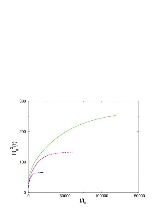
Figure 6: $R_{g}(t)$ for chain length N = 256, 512, 1024.

The presence of these two regimes have been shown by the Brownian dynamics simulation (see Sec.III B and Fig.6 in ref.Chang ). It was found that the first regime becomes faster for the larger quenching $\tau$ (see eq.(3)) whereas the second one become slow as the quenching grows (see eq.(6)).

II.2 Swelling

When the solvent quality is changed suddenly from poor to good or $\theta$ - conditions the globule starts to swell. We consider here for brevity a quench from a poor solvent to $\theta$ - solvent conditions and assume that the globule interior always contains enough solvent molecules i.e., the solvent is not very poor ($\tau\leq 0$) . Then one can ignore a specific role of the solvent transport and assure the homogegeneous globule expansion. In this subsection we restrict ourselves to a scaling picture to set up the main time scales by employing an “expanding blob” picture. Let us therefore assume that during the process of expansion the segments on the length of blob size $\xi$ maintain local equilibrium states, whereas on a larger scales the system is no longer in equilibrium.This amounts to the assumption that the initial state of the globule can be described by free energy which is proportional to the number of blobs times the thermal energy Gennes . We can then write the free energy for the overall quasi - equilibrium regime in the following form

$$F_{\rm glob}\propto k_{B}T\left(\frac{N}{g}\right)\quad,$$ (7)

where the number of monomers in the blob, $g$, is a time dependent function and still has a Gaussian statistics, i.e.

$$g\propto\left(\frac{\xi}{b}\right)^{2}\quad.$$ (8)

We assume as well that the quasi - equilibrium scaling for the overall globule size, $R$, is valid and gives

$$R\propto\xi\left(\frac{N}{g}\right)^{1/3}\quad.$$ (9)

The substitution of eqs.(8) and (9) in eq. (7) yields

$$F_{\rm glob}\propto k_{B}T\frac{b^{6}N^{3}}{R^{6}}\quad.$$ (10)

To take into account the correct long time limiting behavior, when the chain size becomes proportional to $b^{2}N$, the elastic energy term should be included. This term counterbalances the over-swelling and stabilizes the system, so that the whole quasi - equilibrium free energy reads

$$F\propto k_{B}T\left(\frac{b^{6}N^{3}}{R^{6}}+\frac{R^{2}}{b^{2}N}\right)\quad.$$ (11)

After that the corresponding equation of motion for $R(t)$, i.e.

$$\zeta\frac{dR}{dt}=-\frac{\delta F}{\delta R}$$ (12)

takes the following form

$$\frac{N}{D}\frac{dR(t)}{dt}=\frac{b^{6}N^{3}}{R^{7}}-\frac{R}{b^{2}N}\quad.$$ (13)

In eq.(12) $\zeta\sim\zeta_{0}N$ is the Rouse friction coefficient and in eq.(13) $D=k_{B}T/\zeta_{0}$ denotes the monomer diffusion constant. It should be noted, that we do not use the Rouse diffusion constant throughout the paper, since we wish to keep track of the chain length dependences explicitly.

The solution of eq.(13) is

$$R^{2}(t)=\left[R_{0}^{8}e^{-8Dt/b^{2}N^{2}}+b^{8}N^{4}\left(1-e^{-8Dt/b^{2}N^{2}}\right)\right]^{1/4}\quad.$$ (14)

In the asymptotic limit of $t\rightarrow\infty$, we recover the Gaussian chain size, $R^{2}_{\infty}=b^{2}N$. The characteristic time for swelling is determined by the condition: $R_{g}^{2}\sim t^{1/2}_{\rm swell}\sim b^{2}N$. The characteristic time $t^{*}_{\rm swell}$ scales with the chain length as

$$t^{*}_{\rm swell}\sim N^{2}.$$ (15)

We will see in Sec.V, devoted to the numerical investigation of the full equation of motion, that because of coupling of different Rouse modes the driving force of the swelling is mainly determined by the large length scale (see e.g. Fig. 7).

In this consideration the chain is treated as “phantom”, notwithstanding the effective interaction is taken into account through the virial coefficients segments still can cross each other.This use of pseudo potentials does not allow to include topological effects discussed recently. If, however, the effects of topological constraints are dominant, the chain can be swollen only by reptation through the channels made of neighboring segments. The swelling process of an entangled globule needs more consideration Nechaev ; Rabin .

II.3 Effective Hamiltonians and local time scales

The scaling shows what can be expected at large length scales only. It is at first sight difficult to estimate the expected time scales on the level of Rouse type modes. Nevertheless some remarks to the scale dependence on the relaxation modes can be drawn. In the more detailed theory, which is presented below one can recover the dynamical scales on the very late relaxation regimes. The chain size in globular states scales as $R\simeq b(N/\tau)^{1/d}$ for scales larger than the thermal blob size $\xi_{\rm T}=b/\tau$. A general staring point is the Edwards Hamiltonian $H({{\bf R}(s)})$, where ${\bf R}(s)$ defines the chain position vectors and $s$ the contour variable. Any dynamic theory can be formulated through the Rouse modes which are usually defined by a Fourier transform of the position vectors as ${\bf X}(p)=(1/N)\sum_{s}{\bf R}(s)\exp(isp)$, where $p$ stands for the Rouse modes with $p=2\pi n/N$ and $n=0,1,2,\dots,N-1$ Doi . In general the effective Hamiltonian for a collapsed chain can be written in terms of Rouse modes as a simple quadratic form

$$H_{\rm eff}=k_{\rm B}Tf(\tau)\sum_{p}p^{2a}|{\bf X}(p)|^{2}\quad,$$ (16)

where $a$ is determined by the static correlation and the function $f(\tau)$ is 1 for the good and $\theta$ - solvents but $f(\tau)\sim\tau^{2/d}$ for poor solvent conditions. In the case of extended chains it is easy to show that $2a=1+2\nu$ ( where $\nu=3/(d+2)$) whereas in the case of compact chains $2a=1+2/d$. The Rouse dynamics for these effective chain variables ${\bf X}(p)$ is determined by an Rouse equation of the form

$$\zeta_{0}\frac{\partial{\bf X}(p)}{\partial t}+\frac{3k_{\rm B}T}{b^{2}}f(\tau)p^{2a}{\bf X}(p)=0$$ (17)

This effective Rouse equation set the time scales for the latest stages of the dynamical evolution. Namely, for the swelling the relaxation spectrum has the form

$$\tau_{\rm rel}(p)\simeq\frac{\zeta_{0}}{p^{1+2\nu}}\quad,$$ (18)

whereas for the collapse it is

$$\tau_{\rm rel}(p)\simeq\frac{\zeta_{0}}{\tau^{2/d}p^{1+2/d}}\quad.$$ (19)

This corresponds naturally to the characteristic Rouse relaxation times as we will discuss below in more refined theories it in Sec. IVB.

III Equation of motions for correlators

III.1 Model

In this section we provide a more general formulation of the Langevin dynamics for a polymer chain immersed in the solvent. The chain conformation is characterized by the $d$ - dimensional vector - function ${\bf R}(s,t)$ of the time $t$ and $s$ ($1\leq s\leq N$), the segment position along the chain contour. The corresponding intra chain Hamiltonian has the following form

$$H=\frac{1}{2}\epsilon\sum_{s=1}^{N}\left[\nabla_{s}{\bf R}(s,t)\right]^{2}+H_{\rm int}\left\{{\bf R}(s,t)\right\}\quad,$$ (20)

where $\epsilon=dk_{B}T/b^{2}$ is the elastic modulus with the Kuhn segment length $b$, $N$ is the general number of segments and the finite difference $\nabla_{s}{\bf R}_{j}(s,t)={\bf R}_{j}(s+1,t)-{\bf R}_{j}(s,t)$ and the intra-chain interaction Hamiltonian has the form

$$H_{\rm int}\left\{{\bf R}(s,t)\right\} = \frac{1}{2}\sum_{s=1}^{N}\sum_{s^{\prime}=1}^{N}v({\bf R}(s,t)-{\bf R}(s^{\prime},t))$$ (21)

$$+ \frac{1}{3!}\sum_{s=1}^{N}\sum_{s^{\prime}=1}^{N}\sum_{s^{\prime\prime}=1}^{N}w({\bf R}(s,t)-{\bf R}(s^{\prime},t);{\bf R}(s^{\prime},t)-{\bf R}(s^{\prime\prime},t))+\dots$$

In eq.(21) $v({\bf r})$ and $w({\bf r}_{1},{\bf r}_{2})$ are the second and the third virial coefficients correspondingly. Let us treat the low - molecular solvent molecules as a separate component and specify their local positions by the vector - function ${\bf r}^{(p)}(t)$, where $p=1,2,\dots M$ numerates the number of the solvent molecules. We denote by $V_{\rm ps}({\bf r})$ and $V_{\rm ss}({\bf r})$ the polymer - solvent and solvent - solvent interaction potential correspondingly. After that the whole polymer - solvent dynamics is described by the following Langevin equations:

$$\zeta_{0}\frac{\partial}{\partial t}R_{j}(s,t) - \epsilon\Delta_{s}R_{j}(s,t)+\frac{\delta}{\delta R_{j}(s,t)}H_{\rm int}\left\{{\bf R}(s,t)\right\}$$ (22)

$$+ {\frac{\delta}{\delta R_{j}(s,t)}\sum_{p=1}^{M}V_{\rm ps}\left({\bf R}(s,t)-{\bf r}^{(p)}(t)\right)}=f_{j}(s,t)$$

and

$$\zeta^{\prime}_{0}\frac{\partial}{\partial t}r_{j}^{(p)}(t) + \frac{\delta}{\delta r_{j}^{(p)}(t)}\sum_{m=1}^{M}V_{\rm ss}\left({\bf r}^{(p)}(t)-{\bf r}^{(m)}(t)\right)$$ (23)

$$+ \frac{\delta}{\delta r_{j}^{(p)}(t)}\sum_{s=1}^{N}V_{\rm ps}\left({\bf r}^{(p)}(t)-{\bf R}(s,t)\right)={\tilde{f}}_{j}^{(p)}(s,t)\quad,$$

where $j$ numerates Cartesian components, $\zeta_{0}$ and $\zeta^{\prime}_{0}$ are bare friction coefficients of polymer segments and solvent molecules (which should be of the same order and are put equal in the following) and the second order finite difference $\Delta_{s}R_{j}(s,t)=R_{j}(s+1,t)+R_{j}(s-1,t)-2R_{j}(s,t)$.

In order to reformulate the Langevin problem (22) - (23) in a more convenient form we go to the MSR - functional integral representation Rost1 . The generating functional (GF) of the problem has the form

$$Z\left\{\cdots\right\} = \int DR_{j}(s,t)D{\hat{R}}_{j}(s,t)$$ (24)

$$\times \exp\left\{\Xi\left[{\bf R}(s,t),\hat{\bf R}(s,t)\right]+A_{\rm intra}\left[{\bf R}(s,t),\hat{\bf R}(s,t)\right]\right\}\quad,$$

where the influence functional (which describes the influence of solvent molecules on the chain) reads

$$\Xi\left[{\bf R},{\bf\hat{R}}\right] = \ln\int\prod_{p=1}^{M}D{\bf r}^{(p)}(t)D\hat{\bf r}^{(p)}(t)\exp\Bigg{\{}A_{\rm solvent}\left[{\bf r}^{(p)},\hat{\bf r}^{(p)}\right]$$ (25)

$$+ \sum_{p=1}^{M}\sum_{s=1}^{N}\int dti\hat{R}_{j}(s,t)\frac{\delta}{\delta R_{j}(s,t)}V_{\rm ps}\left({\bf R}(s,t)-{\bf r}^{(p)}(t)\right)$$

$$+ \sum_{p=1}^{M}\sum_{s=1}^{N}\int dti\hat{r}_{j}^{(p)}(t)\frac{\delta}{\delta r_{j}^{(p)}(t)}V_{\rm ps}\left({\bf r}^{(p)}(t)-{\bf R}(s,t)\right)\Bigg{\}}\quad,$$

the intra-chain action is given by

$$A_{\rm intra}\left[{\bf R}(s,t),{\hat{\bf R}}(s,t)\right] = \sum_{s=1}^{N}\int dt\Bigg{\{}i{\hat{R}}_{j}(s,t)\left[\zeta_{0}\frac{\partial}{\partial t}R_{j}(s,t)-\epsilon\Delta_{s}R_{j}(s,t)\right]$$ (26)

$$+ \frac{\delta}{\delta R_{j}(s,t)}H_{\rm int}\left\{R_{j}(s,t)\right\}+k_{B}T\zeta_{0}\left[i{\hat{R}}_{j}(s,t)\right]^{2}\Bigg{\}}$$

and the solvent action has the form

$$A_{\rm solvent}\left[{\bf r}^{(p)}(t),{\hat{\bf r}}^{(p)}(t)\right] = \sum_{p=1}^{M}\int dt\Bigg{\{}i{\hat{r}}^{(p)}_{j}(t)\left[\zeta_{0}\frac{\partial}{\partial t}r^{(p)}_{j}(t)+\sum_{m=1}^{M}\frac{\delta}{\delta r^{(p)}_{j}(t)}V\left[{\bf r}^{(p)}(t)-{\bf r}^{(m)}(t)\right]\right]$$ (27)

$$+ k_{B}T\zeta_{0}\left[i{\hat{r}}^{(p)}_{j}(t)\right]^{2}\Bigg{\}}.$$

The representation (24) - (27) is a suitable starting point for further approximations. In particular these expressions are very convenient for integration over collective solvent variables, which will leads to the effective ”actions” for the polymer. We remind that this procedure is only possible if the solvent particles dynamics is much faster compared to the polymer dynamics. While this is in general ensured for long chains, nevertheless this point has to be treated with a care for the polymer collapse problem.

III.2 Self - consistent Hartree approximation

As mentioned already it is an important to point out how the solvent dynamics is treated. Indeed we may follow at least two different ways. The solvent can be considered within the hydrodynamic approximation in the same way as it was done in ref. Fredrick , where the solvent dynamics was described by an incompressible Navier - Stokes liquid. This approach leads to a time - dependent hydrodynamics interaction. The other way is to treat the solvent as a dynamical background in a random phase approximation (RPA). Here we restrict ourselves to the dynamical RPA Rost1 ; Rost2 which is well known in low molecular liquid dynamics Boon . It is also known Boon that the RPA is a mean field type description in which the free - particle behavior is modified by an effective interaction. The main drawback of this approximation is that it does not give the proper hydrodynamic behavior. The reason for this lies in the fact that RPA neglects collisions which dominate in the hydrodynamic regime. We will come to this point in a future publication.

In order to accomplish the calculation for the present purpose we make use of the the transformation to the collective solvent density Rost1 and integrate them out. The level of this procedure will determine the level of approximation also. We relegate all technical details of this calculation in the Appendix A.

The Hartree approximation will then take into account all mean field diagrams. Naturally the mean field description appears poor in good solvent conditions, but becomes better in the globule state, since fluctuations are less important under the increasing globule density.

The GF which is determined by eqs.(74) and (75) is still highly nonlinear with respect to ${\bf R}(s,t)$ and $\hat{\bf R}(s,t)$. In order to handle the difficulties which are associated to these we use Hartree - type approximation. In this approximation the real MSR - action is replaced by the Gaussian one in such a way that all terms which include more than two fields ${\bf R}(s,t)$ and $\hat{\bf R}(s,t)$ ) are written in all possible ways as products of pairs of ${\bf R}(s,t)$ or/and $\hat{\bf R}(s,t)$ coupled to the self - consistent averages of the remaining fields. In ref. Rost3 it was shown that if the number of field components is large the Hartree approximation and the next to the saddle point approximation merge and both become exact. The resulting Hartree action is a Gaussian functional with coefficients which could be represented in terms of correlation and response functions. All calculations are straightforward and details can be found in the Appendix B of ref. Rehkopf . The only difference is that here the second and third virial terms (two last terms in eq.(75)) explicitly enter into the equation. After the collection all terms the final GF reads

$$Z\{\cdots\} = \int D{\bf R}D{\hat{\bf R}}\exp\Big{\{}A_{\rm intra}^{(0)}[{\bf R},{\hat{\bf R}}]$$ (28)

$$+ \sum_{s=1}^{N}\sum_{s^{\prime}=1}^{N}\int_{-\infty}^{\infty}dt\int_{-\infty}^{t}dt^{\prime}\>i{\hat{R}}_{j}(s,t)R_{j}(s^{\prime},t^{\prime})\lambda(s,s^{\prime};t,t^{\prime})$$

$$- \sum_{s=1}^{N}\sum_{s^{\prime}=1}^{N}\int_{-\infty}^{\infty}dt\int_{-\infty}^{t}dt^{\prime}\>i{\hat{R}}_{j}(s,t)R_{j}(s^{\prime},t)\lambda(s,s^{\prime};t,t^{\prime})$$

$$+ \frac{1}{2}\int_{-\infty}^{\infty}dt\int_{-\infty}^{\infty}dt^{\prime}\>i{\hat{R}}_{j}(s,t)i{\hat{R}}_{j}(s^{\prime},t^{\prime})\chi(s,s^{\prime};t,t^{\prime})\Big{\}}\quad,$$

where

$$\lambda(s,s^{\prime};t,t^{\prime}) = \frac{1}{d}G(s,s^{\prime};t,t^{\prime})\int\frac{d^{d}k}{(2\pi)^{d}}k^{4}|V_{\rm ps}({\bf k})|^{2}F({\bf k};s,s^{\prime};t,t^{\prime})S_{00}({\bf k};t,t^{\prime})$$ (29)

$$- \int\frac{d^{d}k}{(2\pi)^{d}}k^{2}\left[|V_{\rm ps}({\bf k})|^{2}S_{01}({\bf k};t,t^{\prime})-V_{\rm ps}({\bf k})\delta(t-t^{\prime})\right]F({\bf k};s,s^{\prime};t,t^{\prime})$$

$$+ \sum_{s^{\prime\prime}=1}^{N}\int\frac{d^{d}kd^{d}q}{(2\pi)^{2d}}w({\bf k},{\bf q})F({\bf q};s^{\prime},s^{\prime\prime};t,t)F({\bf k};s,s^{\prime};t,t)\delta(t-t^{\prime})$$

and

$$\chi(s,s^{\prime};t,t^{\prime})=\int\frac{d^{d}k}{(2\pi)^{d}}k^{2}|V({\bf k})|^{2}F({\bf k};s,s^{\prime};t,t^{\prime})S_{00}({\bf k};t,t^{\prime}).$$ (30)

In eqs.(28) - (30) the response function

$$G(s,s^{\prime};t,t^{\prime})=\left<i{\hat{\bf R}}(s^{\prime},t^{\prime}){\bf R}(s,t)\right>$$ (31)

and the chain density correlator

$$F({\bf k};s,s^{\prime};t,t^{\prime})=\exp\left\{-\frac{k^{2}}{d}Q(s,s^{\prime};t,t^{\prime})\right\}$$ (32)

with

$$Q(s,s^{\prime};t,t^{\prime})\equiv\left<{\bf R}(s,t){\bf R}(s,t)\right>-\left<{\bf R}(s,t){\bf R}(s^{\prime},t^{\prime})\right>\quad.$$ (33)

In eqs.(28) - (30) $S_{00}({\bf k};t,t^{\prime})$ and $S_{01}({\bf k};t,t^{\prime})$ are the solvent RPA - density correlation and response functions correspondingly (see eqs.(76) and (77) in the Appendix A). They embody information on the solvent dynamics.

The pointed brackets denote the self - consistent averaging with the Hartree - type GF, eq.(28). Below we will also concern transient time regimes, so that keeping both time arguments for correlator $F$ in eq.(29) equal to each other does not necessarily mean that this is a static correlator $F_{\rm st}$. On the other hand we assume that the fluctuation - dissipation theorem (FDT) hold for both chain and solvent correlators, then

$$G(s,s^{\prime};t-t^{\prime})=(k_{B}T)^{-1}\frac{\partial}{\partial t^{\prime}}Q(s,s^{\prime};t-t^{\prime})\>\>\>\>{\rm at}\>\>\>t>t^{\prime}$$ (34)

$$S_{01}({\bf k};t-t^{\prime})=(k_{B}T)^{-1}\frac{\partial}{\partial t^{\prime}}S_{00}({\bf k};t-t^{\prime})\>\>\>\>{\rm at}\>\>\>t>t^{\prime}.$$ (35)

Note that in eq.(35) the units of the correlation function $S_{00}$ and the response function $S_{01}$ are different (see the corresponding Appendix A for the notation).

Now we can use eqs.(34) and (35) in eqs.(28) - (33). After integration by parts with respect to time argument $t^{\prime}$, we obtain

$$Z\{\cdots\} = \int D{\bf R}D{\hat{\bf R}}\exp\Big{\{}\sum_{s,s^{\prime}=1}^{N}\int_{-\infty}^{\infty}dt\int_{-\infty}^{t}dt^{\prime}\>i{\hat{R}}_{j}(s,t)\left[\zeta_{0}\delta(t-t^{\prime})+\theta(t-t^{\prime})\Gamma(s,s^{\prime};t,t^{\prime})\right]\frac{\partial}{\partial t}R_{j}(s^{\prime},t^{\prime})$$ (36)

$$- \sum_{s,s^{\prime}=1}^{N}\int_{-\infty}^{\infty}dt\int_{-\infty}^{t}dt^{\prime}\>i{\hat{R}}_{j}(s,t)\>\Omega(s,s^{\prime};t)\>R_{j}(s^{\prime},t)$$

$$+ k_{B}T\sum_{s,s^{\prime}=1}^{N}\int_{-\infty}^{\infty}dt\int_{-\infty}^{\infty}dt^{\prime}\>i{\hat{R}}_{j}(s,t)\left[\zeta_{0}\delta(t-t^{\prime})+\theta(t-t^{\prime})\Gamma(s,s^{\prime};t,t^{\prime})\right]i{\hat{R}}_{j}(s^{\prime},t^{\prime})\Big{\}}\quad,$$

where the memory function

$$\Gamma(s,s^{\prime};t)=\frac{1}{k_{B}T}\int\frac{d^{d}k}{(2\pi)^{d}}\>k^{2}|V_{\rm ps}({\bf k})|^{2}F({\bf k};s,s^{\prime};t)S_{00}({\bf k},t)$$ (37)

and the effective elastic susceptibility

$$\Omega(s,s^{\prime};t) = \epsilon\delta_{\rm ss^{\prime}}\Delta_{\rm s}-\int\frac{d^{d}k}{(2\pi)^{d}}\>k^{2}{\cal V}({\bf k})\left[F({\bf k};s,s^{\prime};t,t)-\delta_{\rm ss^{\prime}}\sum_{s^{\prime\prime}=1}^{N}F({\bf k};s,s^{\prime\prime};t,t)\right]$$ (38)

$$- \frac{1}{2}\sum_{s^{\prime\prime}=1}^{N}\int\frac{d^{d}kd^{d}q}{(2\pi)^{2d}}\>k^{2}w({\bf k},{\bf q})$$

$$\times \left[F({\bf k};s,s^{\prime};t,t)F({\bf q};s^{\prime\prime},s^{\prime};t,t)-\delta_{\rm ss^{\prime}}\sum_{s^{\prime\prime\prime}=1}^{N}F({\bf k};s,s^{\prime\prime\prime};t,t)F({\bf q};s^{\prime\prime\prime},s^{\prime\prime};t,t)\right]\quad.$$

In eq.(38) the Fourier components of the effective segment - segment self - interaction function is given by

$${\cal V}({\bf k})=v(k)-\frac{|V_{\rm ps}({\bf k})|^{2}\Phi_{\rm st}({\bf k})/k_{B}T}{1+V_{\rm ss}({\bf k})\Phi_{\rm st}({\bf k})/k_{B}T}\quad,$$ (39)

where $\Phi_{\rm st}({\bf k})$ is the static density correlator for the free solvent system. In eq.(39) the second term results from a coupling with solvent degree of freedom. The memory function (37) describes the renormalization of the Stokes friction coefficient $\zeta_{0}$ which originates from a coupling between polymeric and solvent fluctuations. The effective elastic susceptibility, eq.(38), gives an account of the non - dissipative contributions, which arises not only from the local spring - interaction (the first term in eq.(38)) but also from effective two and three point interactions.

III.3 Equation of motion

Now we are in a position to derive equation of motion for the time - displaced correlator

$$C(s,s^{\prime};t,t^{\prime})=\left<{\bf R}(s,t){\bf R}(s^{\prime},t^{\prime})\right>$$ (40)

as well as for the equal - time correlator

$$P(s,s^{\prime};t)=\left<{\bf R}(s,t){\bf R}(s^{\prime},t)\right>\quad.$$ (41)

The standard way to derive equations of motion by starting from the Hartree action (see eq.(28) is discussed in Appendix B ref.Horner . Using this way for the Hartree action in eq.(28) and taking into account FDT yields

$$\zeta_{0}\frac{\partial}{\partial t}C(s,s^{\prime};t,t^{\prime}) - \sum_{m=1}^{N}\>\Omega(s,m;t)C(m,s^{\prime};t,t^{\prime})$$ (42)

$$+ \sum_{m=1}^{N}\int_{t^{\prime}}^{t}\>\Gamma(s,m;t,\tau)\frac{\partial}{\partial\tau}C(m,s^{\prime};\tau,t^{\prime})d\tau=-2k_{B}T\zeta_{0}G(s^{\prime},s;t^{\prime},t)\quad.$$

In the case of $t^{\prime}<t$ the r.h.s. of eq.(42) is zero and the time - displaced correlator satisfies the equation

$$\zeta_{0}\frac{\partial}{\partial t}C(s,s^{\prime};t,t^{\prime})-\sum_{m=1}^{N}\>\Omega(s,m;t)C(m,s^{\prime};t,t^{\prime})+\sum_{m=1}^{N}\int_{t^{\prime}}^{t}\>\Gamma(s,m;t,\tau)\frac{\partial}{\partial\tau}C(m,s^{\prime};\tau,t^{\prime})d\tau=0\quad.$$ (43)

In order to derive the equation for the equal - time correlator (41) we recall that

$$\frac{\partial}{\partial t}P(s,s^{\prime};t)=\left[\frac{\partial}{\partial t}C(s,s^{\prime};t,t^{\prime})\right]_{t^{\prime}=t}+\left[\frac{\partial}{\partial t^{\prime}}C(s,s^{\prime};t,t^{\prime})\right]_{t^{\prime}=t}$$ (44)

and the initial condition Rehkopf

$$\zeta_{0}G(s,s^{\prime};t+0^{+},t^{\prime})=-d\delta(s-s^{\prime})\quad.$$ (45)

Let us make the permutation of time moments, $t{\to\atop\leftarrow}t^{\prime}$, in eq. (42). Combining this equation with the original one and using eqs. (44) - (45) in the limit $t=t^{\prime}+\epsilon$ at $\epsilon\to 0$, one can derive the result:

$$\frac{1}{2}\zeta_{0}\frac{\partial}{\partial t}P(s,s^{\prime};t)-\sum_{m=1}^{N}\>\Omega(s,m;t)P(s,s^{\prime};t)=dk_{B}T\delta(s-s^{\prime})$$ (46)

It is of interest that in eq.(46) the memory term is dropped out.

As it was discussed in the Introduction , here we restrict ourselves to the case where the translational invariance along the chain backbone holds during the collapse (swelling). Generally speaking, the presence of the “pearl necklace” structure breaks down this invariance, so that the correlator $P(s,s^{\prime};t)$ depends not only on the “chemical distance” $|s-s^{\prime}|$ but also on the position along the chain backbone. Even the interface might violate this invariance because the chain segments on the surface and in the bulk experience quite different environment. Nevertheless, in the case when the pearl formation is fast compared to the dynamics of the envelop and there positions along the chain are random these differences can be averaged out (by preparing an appropriate ensemble of pearls realizations) and the effective invariance still holds. In this situation the Rouse components are the “good variables” and it is worthwhile to make the Rouse transformation in the standard way Doi :

$${\bf X}(p,t)=\frac{1}{N}\sum_{s=1}^{N}{\bf R}(s,t)\exp(isp)$$ (47)

and

$${\bf R}(s,t)=\sum_{p=0}^{2\pi}{\bf X}(p,t)\exp(-isp)\quad,$$ (48)

where the Rouse mode $p=2\pi n/N$ at $n=0,1,\dots,N-1$ and we have used for simplicity the cyclic boundary conditions. After that the eq.(46) reads

$$(2D)^{-1}\frac{\partial}{\partial t}P(p;t)+\Omega(p;t)P(p;t)=dN^{-1}\quad,$$ (49)

where $D=k_{B}T/\zeta_{0}$ is the bare diffusion coefficient and

$$\Omega(p;t) = \frac{2d}{b^{2}}(1-\cos p)+\frac{N}{k_{B}T}\>\int\frac{d^{d}k}{(2\pi)^{d}}\>k^{2}{\cal V}({\bf k})\left[F({\bf k};p;t,t)-F({\bf k};p=0;t,t)\right]$$ (50)

$$+ \frac{N^{2}}{2k_{B}T}\>\int\frac{d^{d}kd^{d}q}{(2\pi)^{2}d}\>k^{2}w({\bf k},{\bf q})\Big{[}F({\bf k};p;t,t)F({\bf q};p=0;t,t)$$

$$- F({\bf k};p=0;t,t)F({\bf q};p=0;t,t)\Big{]}\quad.$$

On the other hand, the Rouse transformation of the chain density correlator has the form

$$F({\bf k};p;t,t)=\frac{1}{N}\sum_{n=1}^{N}\cos(pn)\exp\left\{-\frac{k^{2}}{d}Q(n;t,t)\right\}\quad.$$ (51)

For the short range segment - segment interaction one can neglect the wave vector dependence in ${\cal V}$ and $w({\bf k},{\bf q})$ by putting ${\cal V}\approx v$ and $w({\bf k},{\bf q})\approx w$. Using eq.(51) in eq.(50) and performing the integration over ${\bf k}$ and ${\bf q}$ yields

$$\Omega(p;t) = \frac{2d}{b^{2}}(1-\cos p)-v\frac{d^{\frac{d}{2}+2}}{2k_{B}T(4\pi)^{\frac{d}{2}}}\sum_{n=1}^{N}\>\frac{1-\cos(pn)}{\left[Q(n,t)\right]^{\frac{d+2}{2}}}$$ (52)

$$- w\frac{d^{d+2}}{4k_{B}T(4\pi)^{d}}\sum_{n=1}^{N}\sum_{m=1}^{N-n}\>\frac{1-\cos(pn)}{\left[Q(n,t)\right]^{\frac{d+2}{2}}\left[Q(n,t)\right]^{\frac{d}{2}}}\quad.$$

We stress that the equation of motion (49), (52) for $P(p;t)$ is highly nonlinear because the correlator $Q(n,t)$ depends on all other $P(\kappa;t)$ (which provides also a Rouse mode coupling) as follows

$$Q(n,t) = P(n,n;t)-P(n,0;t)$$ (53)

$$= \sum_{\kappa=2\pi/N}^{2\pi}\>\left[1-\cos(\kappa n)\right]P(\kappa;t)$$

In equilibrium all equal - time correlators in eqs.(52) - (53) can be seen as static ones: $P(p;t)\to C_{\rm st}(p)$ and $Q(n,t)\to Q_{\rm st}(p)$. Using this limit in eq.(49) leads to the following equilibrium equation

$$\left[NC_{\rm st}(p)\right]^{-1} = \frac{2}{b^{2}}(1-\cos p)-v\frac{d^{\frac{d}{2}+1}}{2k_{B}T(4\pi)^{\frac{d}{2}}}\sum_{n=1}^{N}\>\frac{1-\cos(pn)}{\left[Q_{\rm st}(n)\right]^{\frac{d+2}{2}}}$$ (54)

$$- w\frac{d^{d+1}}{4k_{B}T(4\pi)^{d}}\sum_{n=1}^{N}\sum_{m=1}^{N-n}\>\frac{1-\cos(pn)}{\left[Q_{\rm st}(n)\right]^{\frac{d+2}{2}}\left[Q_{\rm st}(n)\right]^{\frac{d}{2}}}\quad.$$

This equation is identical (with the accuracy of prefactors) with the variational (Euler) equation which we have recently discussed in ref.Miglior ; Miglior1 . This provides the means for answering one of the important questions of whether the Edwards Hamiltonian can be equally used for dynamical calculations. Within the Hartree approximation the answer is positive provided that the second and third virial coefficients are considered as free parameters. In fact, the Hartree approximation is a dynamical counterpart of the variational approach Miglior ; Miglior1 .

IV Early and latest stages of the collapse (swelling)

Now we are in a position to consider some limiting cases which allow an analytical investigation. These are obviously very early and latest stages of the transformation. We shall defer the full discussion which based on the equation of motion numerical solution until the next section.

Let us consider the abrupt solvent quality changing between the initial $v_{\rm i}>0$ and the final $v_{\rm f}<0$, which is the case of the collapse experiment. For the swelling case these are the following: $v_{\rm i}<0$ and $v_{\rm f}>0$.

IV.1 Early stages

For the very early stage the eq.(49) can be linearized around the starting state, which leads to the following form

$$(2D)^{-1}\frac{\partial}{\partial t}P(p;t)+\Omega_{\rm st}(p)P(p;t)=dN^{-1}\quad,$$ (55)

where

$$\Omega_{\rm st}(p) = \frac{2d}{b^{2}}(1-\cos p)-v_{\rm f}\frac{d^{\frac{d}{2}+2}}{2k_{B}T(4\pi)^{\frac{d}{2}}}\sum_{n=1}^{N}\>\frac{1-\cos(pn)}{\left[Q_{\rm st}(n)\right]^{\frac{d+2}{2}}}$$ (56)

$$- w\frac{d^{d+1}}{4k_{B}T(4\pi)^{d}}\sum_{n=1}^{N}\sum_{m=1}^{N-n}\>\frac{1-\cos(pn)}{\left[Q_{\rm st}(n)\right]^{\frac{d+2}{2}}\left[Q_{\rm st}(n)\right]^{\frac{d}{2}}}\quad.$$

In the eq.(56) the static correlator $Q_{\rm st}(n)$ should be seen as a coil correlator, i.e. $Q_{\rm st}(n)=Q_{\rm st}^{coil}(n)$ in the case of collapse and as a globule correlator, $Q_{\rm st}(n)=Q_{\rm st}^{glob}(n)$, in the case of swelling.

Combining eq.(56) with eq.(54), which is valid in the equilibrium at $v=v_{\rm i}$, yields

$$\Omega_{\rm st}(p)=d\left[NC_{\rm st}(p)\right]^{-1}+(v_{\rm i}-v_{\rm f})\frac{d^{\frac{d}{2}+1}}{2T(4\pi)^{\frac{d}{2}}}\sum_{n=1}^{N}\>\frac{1-\cos(pn)}{\left[Q_{\rm st}(n)\right]^{\frac{d+2}{2}}}$$ (57)

The very early stage can be characterized by the initial relaxation rate

$$X(p)\equiv\frac{\partial}{\partial t}P(p;t)\biggr{|}_{t=0}=\left[dN^{-1}-\Omega_{\rm st}(p)C_{\rm st}(p)\right](2D)\quad,$$ (58)

which with the use of eq. (57) can be represented in the following form

$$X(p)=-\frac{(v_{\rm i}-v_{\rm f})}{\zeta_{0}}\>\>C_{\rm st}(p)\>{\cal F}(p)\quad,$$ (59)

where

$${\cal F}(p)=\frac{d^{\frac{d}{2}+2}}{(4\pi)^{\frac{d}{2}}}\sum_{n=1}^{N}\>\frac{1-\cos(pn)}{\left[Q_{\rm st}^{(i)}(n)\right]^{\frac{d+2}{2}}}\quad.$$ (60)

The relaxation law for the decrement of the gyration radius $\Delta R_{g}^{2}(t)=\sum_{p=2\pi/N}^{2\pi}\left[P(p;t)-P(p;0)\right]$ at the early stage takes the form

$$\Delta R_{g}^{2}(t)=-\frac{(v_{\rm i}-v_{\rm f})}{\zeta_{0}}\>\>\Bigl{[}\sum_{p=2\pi/N}^{2\pi}C_{\rm st}(p)\>{\cal F}(p)\Bigr{]}\>t\quad.$$ (61)

Taking into account the asymptotic behavior, $\left[C_{\rm st}(p)\right]^{-1}\propto p^{1+2\nu}$ (for small $p$), $Q_{\rm st}(n)\propto n^{2\nu}$ (for large $n$), where $\nu$ is the Flory exponent, one can obtain for function ${\cal F}(p)$ the following scaling

$${\cal F}(p)\propto p^{\nu(d+2)-1}$$ (62)

For the collapse case $v_{\rm i}>v_{\rm f}$. For quenching from the good solvent, $\nu=3/(d+2)$, and ${\cal F}_{c}(p)\propto p^{2}$, whereas for the quenching from the $\theta$ - solvent $\nu=1/2$ and ${\cal F}_{c}(p)\propto p^{d/2}$.

In the case of swelling $v_{\rm i}<v_{\rm f}$. If one heat up the system starting from the globule state then $\nu=1/d$ and ${\cal F}_{s}(p)\propto p^{2/d}$, whereas for the $\theta$ - solvent initial state one has ${\cal F}_{s}(p)\propto p^{d/2}$.

We will leave the discussion of the relaxation rate $X(p)$ till the next section but one can immediately see that $X(p)$ has the following scaling forms. For collapse

$$X_{c}(p)\propto-\frac{v_{\rm i}-v_{\rm f}}{\zeta_{0}}\left\{\begin{array}[]{l@{\quad,\quad}l}1/p^{(4-d)/(d+2)}&{\rm good-solvent}\\ 1/p^{2-d/2}&\theta-{\rm solvent}\end{array}\right.$$ (63)

where the first and the second lines refer to the quenching from the good and $\theta$ - solvents correspondingly.

For the swelling process we find respectively for different initial starting points

$$X_{s}(p)\propto\frac{v_{\rm f}-v_{\rm i}}{\zeta_{0}}\left\{\begin{array}[]{l@{\quad,\quad}l}1/p&{\rm poor-solvent}\\ 1/p^{2-d/2}&\theta-{\rm solvent}\end{array}\right.$$ (64)

Here the first and the second lines are assigned to the heating up from the poor and $\theta$ - solvents correspondingly.

IV.2 Latest stages

Now the system is close to the globule state (if the collapse is under discussion) and we can linearize the equation of motion around it. In this case eq.(55) is still valid but $\Omega_{\rm st}(p)$ should be calculated in the globule state, which comes out of eq.(56) after substitution $Q_{\rm st}(n)\to Q_{\rm st}^{(gl)}(n)$. In its turn correlator for the globule state $Q_{\rm st}^{(gl)}(n)$ satisfies the eq.(54) at $v=v_{\rm f},C_{\rm st}(p)=C_{\rm st}^{(gl)}(p)$ and $Q_{\rm st}(n)=Q_{\rm st}^{(gl)}(n)$. After simple calculations one can obtain

$$\Omega_{\rm st}^{(gl)}(p)=d\left[NC_{\rm st}^{(gl)}(p)\right]^{-1},$$ (65)

where $\left[NC_{\rm st}^{(gl)}(p)\right]^{-1}\propto p^{1+2/d}$. On the latest stage only the relaxation mode $p=2\pi/N$ contributes. Then for $\Delta r_{g}^{2}(t)=R_{g}^{2}(t)-R_{g}^{2}(\infty)$ we have

$$\Delta r_{g}^{2}(t)\propto\exp\left\{-2D\>\Omega_{\rm st}^{(gl)}\left(p=\frac{2\pi}{N}\right)\>t\right\}\quad,$$ (66)

i.e. the characteristic relaxation time is given by

$$\tau_{\rm rel}\propto\frac{1}{D}N^{1+2/d}\quad,$$ (67)

which agrees with ref. Pitard1 . Note that we derived this behavior as well previously when we had used the effective Hamiltonian for the collapsed chain. Obviously these crude estimated describe already the main issues of the dynamic behavior.

The same remark holds for the case of the large time limit for the swelling in a good solvent ($v_{f}>0$). The formal dynamic theory describes these mode dependence as

$$\tau_{\rm rel}\propto\frac{1}{D}N^{\frac{d+8}{d+2}}\quad,$$ (68)

which is also consistent with ref.Pitard1 . Again we derived this already by the effective chain Hamiltonian in Sec. IIC.. Physically this appears naturally since the choice of the exponent in eq.(16) uses implicitly the FDT to determine the statics correctly. It is interesting that eqs.(67) and eqs.(68) can be seen as a characteristic Rouse time, $\tau_{\rm Rouse}\sim N^{1+2\nu}$ (see e.g.PGG ), where the Flory exponent $\nu=1/d$ or $\nu=3/(d+2)$ in the case of eqs.(67) (collapse) and eqs.(68) (swelling in a good solvent) correspondingly.

V Numerical Studies

V.1 Collapse

To analyze these results in more detail we performed numerical studies of the corresponding equations. We studied so far only the asymptotic behavior, whereas the intermediate time regimes are not accessible. To do so we explicitly computed the numeric solution of Eq. 49 for chain length $N=2^{6}-2^{10}$. For the whole procedure, the three body interaction term is fixed as $v_{3}=b^{6}\equiv 1$. The time scale is measured in units of $t_{0}=\zeta_{0}b^{2}/k_{B}T$. The monomer density in a globule is determined by the balance between the two-body attraction and three body repulsion, $\rho=|v_{2}|/v_{3}=-\tau/b^{3}$. The excluded volume provides the condition for the maximum density $\rho_{\rm max}|v_{2}|\leq 1$.

As mentioned earlier, the chain is phantom, i.e., we use pseudo-potentials only which might cause a faster collapse since the chain segments are allowed to pass through each other. However, this effect is maybe a minor correction at least in the early stages at the beginning of the collapse. At later stages artifact caused by the phantom assumption (such as an overshooting on the relaxation curves) are expected to be more pronounced. In order to assure the validity of the virial expansion and to minimize these artifacts, the solvent quality should remain in the limit where $v_{2}^{2}/v_{3}\ll 1$. Let us now discuss the results in more detail.

V.1.1 Solvent quality dependence

First we are going to present the dependence on the solvent quality as a first check of the theory. The mean squared radius of gyration $R_{g}^{2}(t)$ for various second virial coefficient $v_{2}$ is plotted in Fig. 2 for $N=512$. Due to the finite size effect the solvent quality which gives the coil to globule transition is expected to be shifted by $\sim 1/\sqrt{N}$. We observe the transition occurs around $\tau\approx-0.25$.

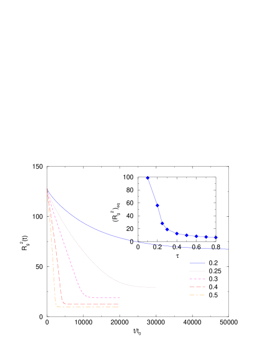
Figure 2: The mean square radius of gyration $R_{g}^{2}(t)$ as a function of time after quench to poor solvent conditions from $\theta$ solvent condition where the chain configuration is Gaussian. The equilibrium $R_{g}^{2}(t)$ is shown in inset for various solvent quality. The coil to globule transition is observed at solvent quality $|\tau|=0.25$.

In equilibrium, the size of the globule in the poor solvent regime varies as $R\sim b(N/|\tau|)^{1/3}$, according to the solvent quality. This is in good agreement with the scaling predictions.

V.1.2 Chain length dependence

The next issue is the chain length dependence. In Fig. 3, the mean square radius of gyration $R^{2}_{g}(t)$ during the collapse is shown for various chain size $N$. The characteristic total collapse time increases linearly as chain length $N$, as predicted from the scaling estimate given by eq.(4).

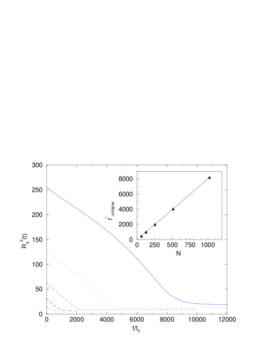
Figure 3: The mean square $R^{2}_{g}(t)$ of various chain length $N$ as a function of time after quench to poor solvent conditions ($\tau=-0.4$) $N=64,128,256,512,1024$ from bottom to top. The inset shows the total characteristic time for collapse for each chain vs. their length $N$.

V.1.3 Relaxation times for individual modes

During the coil - globule transition the collapse occurs in hierarchical patterns, such that the collapsed segment on a smaller length scale can be considered as the unit length of the larger scale of the chain. In the process of the collapse transition the active modes disappear one after another. We expect such a hierarchical collapse to be visible in the corresponding Fourier mode correlator $P(p,t)$ where $p=2\pi n/N$ and $n=1,2,\dots,N-1$. The characteristic time for mode $p$ is related to the relaxation time of the subchain of length $g=N/n$ After the elapse of time $t_{n}$ all length scales less than $g$ are collapsed (see the Sec.II). There exist $N/g$ collapsed sub-chains at a given time and the hierarchically larger length structure is a random walk of these sub-chains. At times less than $t_{n}$, the contractions on length scale smaller than $g$ contribute essentially to the decrease of the correlatator $P(p\sim 1/g,t)$. For times $t>t_{n}$, further contractions from the larger scales are reflected. Indeed, the relaxation behavior of $P(p,t)$ on smaller length scales (or larger $n\geq 2$) shows two clearly distinctive regimes, see Fig. 4. However, the longest mode ($n=1$) shows only a single slope until the chain finds itself in the globular state. We may define the fast decreasing regime as the first characteristic time scale $t_{p}^{*}$ for each mode $p$. The first characteristic time $t_{p}^{*}$ is therefore related to the “internal” relaxation time of subchain of length $g=N/n$. The subchain relaxation time scales with its length $g$ as $t_{p}^{*}\sim g\sim 1/p$ which is consistent with the scaling results (see Sec.IIA). The size of each length scale continue to decrease after time $t_{p}^{*}$ and this is due to the larger scale contraction.

It is now instructive to give a more general estimate for the characteristic time $t_{p}^{*}$. According to eq.(59) the driving force for the collapse transition scales as $f_{p}\sim(v_{\rm i}-v_{\rm f})C_{\rm st}{\cal F}(p)\sim\tau p^{\nu d-2}\sim\tau/g^{\nu d-2}$. In $d=3$ and at $\nu=1/2$, $f_{p}\sim\tau\sqrt{g}$, which agrees with eq.(1). In the same manner as in Sec.IIA, the characteristic time scales as $t_{p}^{*}\sim R/u$ where $R$ describes the chain properties as $R\sim n^{\nu}$ and $u\sim f_{p}/\zeta_{0}g$, so that the resulting scaling reads,

$$t_{p}^{*}\propto\frac{\zeta_{0}}{\tau}\;g^{\nu(1+d)-1}\quad.$$ (69)

For three dimensions, $d=3$ and $\nu=1/2$ we recover the relation, $t_{p}^{*}\sim\zeta_{0}g/\tau$, which is supported by the scaling analysis in the Sec.IIA.

After the time $t_{p}^{*}$, each Fourier mode decreases slowly (for $n>2$). The total collapse time for each mode is identical with that of the first characteristic time for the longest mode, $t_{p=2\pi/N}^{*}$. The slope decrease after time $t_{p}^{*}$ is controlled (because of modes coupling) by the contraction on longer scales (or smaller $p$ modes). The fast relaxation time for the second largest mode for the chain length $N$ coincides with the total collapse time for a chain of the corresponding half length (see again the Sec. II). Naturally, the longest relaxation mode has only one characteristic regime.

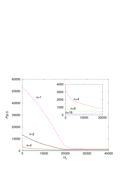
Figure 4: The relaxation of each mode $P(p=2\pi n/N,t)$ during the collapse transition.

V.2 Swelling

We turn now to the the case of swelling and present the numerical results of the globule expanding after a quench from poor to a good (or $\theta$ - solvent) condition. The initial configuration is now assumed to be a compact globule which is prepared by a poor solvent with a certain negative second virial coefficient. Contrary to the collapse dynamics, which based on the hierarchically crumpled fractal picture, the swelling can be conceived as an homogeneous extension of the different Rouse modes.

The time dependence of $P(p,t)$ is shown in Fig. 5 for different values of the mode index $p$. Small length scales (or large $p$) relax fast, in the sense that they are saturated faster, while larger scales grow slower. There is no clear dynamic exponent observed for the subchain relaxation time in the numerical solution. In the beginning of the swelling, overshooting is observed for large $p$ values. This is an obvious artifact of a phantom chain. The monomers move out from the dense globule explosively as soon as the solvent condition is switched to a theta solvent. The phantom chain can pass through surrounding dense phase without being hindered by the topological constraint. The overshooting shows up when the size of the subchain of $g$ monomers $r(g)$ is comparable to the boundary size of the total chain $R(t)$. It appears also that the virial expansion is not simply applicable for at least the early stage of swelling.

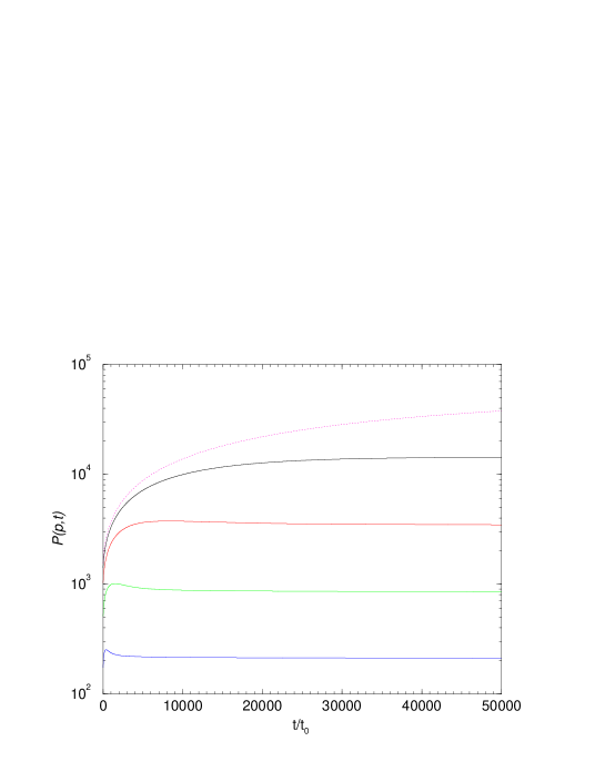
Figure 5: The mode correlation function $P(p,t)$ for each mode $pN/2\pi$=1,2,4,8,16 from top to bottom. The solvent quality is switched from $v_{\rm i}=-0.3b^{3}$ to $v_{\rm f}=-0.1b^{3}$. The chain length is N=1024.

The growth of the overall size $R_{g}^{2}(t)\sim t^{z}$ is also computed. The dynamic exponent is approximately $z\sim 1/2$. The total relaxation time $t^{*}_{swell}$ grows as $N^{2}$ as the chain length increases.

In order to demonstrate how different modes contribute to the swelling, it is useful to calculate the normalized relaxation rate $\overline{X}(p,t)=1-P(p,t)\Omega(p,t)/d$ as a function of wave vector $p$. We have discussed already (see Sec.IV) the asymptotic forms, i.e. at $p\ll 1$, of this function at the initial time moment. In Fig. 7, we compute the relaxation rate $\overline{X}(p,t)$ for the swelling condition. When the system is suddenly quenched to the $\theta$ solvent, the compact globule conformation is unstable and far from the equilibrium. The relaxation rate $X(p,t)$ reflects the discrepancy between the desired conformation and the conformation at given time $t$. If the system tends to the equilibrium, the relaxation rate obviously vanishes. The contribution to the total swelling from different modes $p$ changes as swelling proceeds. The length scales smaller then the blob size do not contribute in the swelling. We may define $p_{\rm max}=2\pi/g$ as the Rouse index of the shortest active mode at $t=0$, where $g$ is again the number of chain units in the Gaussian blob. (The larger $p>p_{\rm max}$ do not contribute). As the chain swells, the size of the boundary is growing, but on the other hand, the position of $p_{\rm max}(t)$ decreases accordingly. In Fig. 7 one can see the shifting of $p_{\rm max}(t)$ to the smaller value of $p$ in the course of time. These findings are consistent with the “expanding blob” picture which we discussed in the Sec.II B.

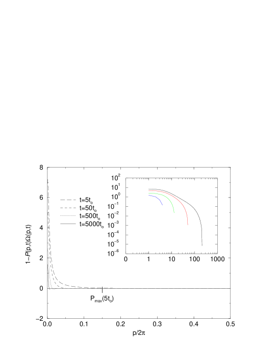
Figure 7: The relaxation rate $1-\Omega(p)P(p)/d$ for half cycle of $p$ with chain length N=1024. The contribution to the swelling comes from each mode $p<p_{c}$ at given time. The positive value regimes are active mode. The inset shows the log-log plot of the relaxation rate.

VI Conclusion

Using the MSR - generating functional technique and the self - consistent Hartree approximation we have derived the equation of motion for the time dependent monomer - to - monomer correlation function. The numerical solutions of this equation for the Rouse modes and the gyration radius $R_{g}$ in the cases of collapse and swelling regimes have been discussed. It has been shown that the simple scaling arguments for the collapse based on the hierarchically crumpled fractal picture match pretty well with our numerical findings. The size of the crumples (or the size of the collapsed segment of the chain) grows successively, so that the characteristic time of the collapse changes linearly with the length of the collapsed segment. Swelling, on the contrary, goes homogeneously, with the Rouse modes relaxing with different relaxation rates. The spectrum of the relaxation rate spans the interval between the minimal $p_{\rm min}=2\pi/N$ and maximal $p_{\rm max}=2\pi/g$ Rouse mode indices, where the “expanding blob” length, $g$, is a growing function of time.

In this paper we have restricted ourselves to the ring polymer. The presence of free ends in the open polymer chain brings some special features mainly on the later stage of the collapse. This question have been discussed in the number of papers abrams01 ; ostrovsky . In particular in ref. abrams01 it has been shown that the late stage configuration consists of two globules with connecting bridge between them (dumb - bell structure). In this case the dynamics is determined by the bridge tension between the globules and the hydrodynamic friction experienced by the globules.

We should stress that the whole consideration ignores up to now two important things: (i) hydrodynamical interaction and (ii) topological (or entanglements) effects. The hydrodynamical interaction can be simply taken into account by treating the solvent as a incompressible Navier - Stokes liquid coupled with chains monomers Fredrick . Within the self - consistent Hartree approximation the effective friction coefficient depends from the monomer - to - monomer correlation function, $Q(n,t)$, so that the closed equation of motion for the Rouse modes correlator can be solved numerically. This point will be discussed in detail in a forthcoming publication.

The systematic inclusion of topological constraints in the dynamics of collapse (or swelling) is a much more complicate theoretical problem. It was argued in ref.Nechaev that at the chain length $N\gg N_{\rm e}$ (where $N_{\rm e}$ is an effective entanglement length) the topological constraints become essential. The self similar process of crumpling which we have discussed in Sec.IIA is restricted also by topological constraints as soon as a collapsed segment is longer then $N_{\rm e}$. These segments have a fixed topology and in a sense are in a partially equilibrium state called “fractal crumpled globule”. The characteristic time of of this first stage of collapse is $t_{\rm collapse}\approx t_{\rm collapse}^{(0)}(1+b^{6}/N_{\rm e}w)$ , where $w$ is a third virial coefficient and $t_{\rm collapse}^{(0)}$ is the collapse time without the topological effects. At the subsequent stage the “crumpled globule” relaxes to the full equilibrium via the penetration of the chain ends through the globule and many knots formation. This stage has a reptational mechanism and as a result the characteristic relaxation time is scaled as $t_{\rm top}\sim N^{3}$. Unfortunately, nowadays it is not quite clear how to incorporate the topological constraints in the equation of motion, so that this is a challenging problem for the future discussion. Finally we can mention as an interesting possible application of our approach the problem of the globule dissolution under an external force Kreitmeier . This problem is also important for the interpretation of the stress - strain relations in polymer networks Cifra .

Appendix A Integration over solvent variables

In order to accomplish the RPA - calculation let us make as usual Rost1 the transformation to the collective solvent density

$$\rho({\bf r},t)=\sum_{p=1}^{M}\>\delta\left({\bf r}-{\bf r}^{(p)}(t)\right)$$ (70)

and response field density

$$\pi({\bf r},t)=\sum_{p=1}^{M}\sum_{j=1}^{d}\>i{\hat{r}}^{(p)}_{j}(t)\nabla_{j}\delta\left({\bf r}-{\bf r}^{(p)}(t)\right)\quad.$$ (71)

These transform the influence functional (25) to the form

$$\Xi\left[{\bf R},{\hat{\bf R}}\right] = \ln\int D\rho({\bf k},t)D\pi({\bf k},t)$$ (72)

$$\times \exp\Bigg{\{}W[\rho,\pi]-\int dt\int\frac{d^{d}k}{(2\pi)^{d}}\pi(-{\bf k},t)\rho({\bf k},t)V_{\rm ss}({\bf k})$$

$$+ \sum_{s=1}^{N}\int dt\>i{\hat{R}}_{j}(s,t)\int\frac{d^{d}k}{(2\pi)^{d}}ik_{j}V_{\rm ps}({\bf k})\rho({\bf k},t)\exp\{i{\bf k}{\bf R}(s,t)\}$$

$$- \sum_{s=1}^{N}\int dt\int\frac{d^{d}k}{(2\pi)^{d}}\pi({\bf k},t)V_{\rm ps}(-{\bf k})\exp\{i{\bf k}{\bf R}(s,t)\}\Bigg{\}}\dots,$$

where the functional $W$ depends only on properties of the free system

$$W\{\rho,\pi\} = \ln\int\prod_{p=1}^{M}D{\bf r}^{(p)}D{\hat{\bf r}}{(p)}\exp\left\{A_{\rm solvent}^{(0)}\left[{\bf r}^{(p)},{\hat{\bf r}}^{(p)}\right]\right\}$$ (73)

$$\times \delta\left(\rho({\bf r},t)-\sum_{p=1}^{M}\>\delta\left({\bf r}-{\bf r}^{(p)}(t)\right)\right)$$

$$\times \delta\left(\pi({\bf r},t)-\sum_{p=1}^{M}\sum_{j=1}^{d}\>i{\hat{r}}^{(p)}_{j}(t)\nabla_{j}\delta\left({\bf r}-{\bf r}^{(p)}(t)\right)\right)\ .$$

Here $A_{\rm solvent}^{(0)}$ is the free solvent action. Following ref. Rost1 ; Rost2 one can expand $W\{\rho,\pi\}$ up to the second order with respect $\rho$ and $\pi$, which formally corresponds to the dynamical RPA. Then the solvent variables in (72) can be integrated over and for GF we obtain the following result

$$Z\left\{\cdots\right\}=\int DR_{j}(s,t)D{\hat{R}}_{j}(s,t)\>\exp\left\{A_{\rm eff}\left[{\bf R}(s,t),\hat{\bf R}(s,t)\right]\right\}\quad,$$ (74)

where

$$A_{\rm eff}\left[{\bf R},{\hat{\bf R}}\right] = A_{\rm intra}^{(0)}\left[{\bf R},{\hat{\bf R}}\right]$$ (75)

$$+ \frac{1}{2}\int_{1}\int_{1^{\prime}}\>i{\hat{R}}_{j}(1)\int\frac{d^{d}k}{(2\pi)^{d}}k_{j}k_{p}|V_{\rm ps}({\bf k})|^{2}\exp\left\{i{\bf k}\left[{\bf R}(1)-{\bf R}(1^{\prime})\right]\right\}i{\hat{R}}_{p}(1^{\prime})S_{00}({\bf k},t-t^{\prime})$$

$$- \int_{1}\int_{1^{\prime}}\>i{\hat{R}}_{j}(1)\int\frac{d^{d}k}{(2\pi)^{d}}ik_{j}|V_{\rm ps}({\bf k})|^{2}\exp\left\{i{\bf k}\left[{\bf R}(1)-{\bf R}(1^{\prime})\right]\right\}S_{01}({\bf k},t-t^{\prime})$$

$$+ \int_{1}\int_{1^{\prime}}\>i{\hat{R}}_{j}(1)\int\frac{d^{d}k}{(2\pi)^{d}}ik_{j}v({\bf k})\exp\left\{i{\bf k}\left[{\bf R}(1)-{\bf R}(1^{\prime})\right]\right\}\delta(t-t^{\prime})$$

$$+ \frac{1}{2}\int_{1}\int_{1^{\prime}}\int_{1^{\prime\prime}}\>{\hat{R}}_{j}(1)\int\frac{d^{d}kd^{d}q}{(2\pi)^{2d}}ik_{j}w({\bf k},{\bf q})$$

$$\times \exp\left\{i{\bf k}\left[{\bf R}(1)-{\bf R}(1^{\prime})\right]+i{\bf q}\left[{\bf R}(1^{\prime})-{\bf R}(1^{\prime\prime})\right]\right\}\delta(t-t^{\prime})\delta(t^{\prime}-t^{\prime\prime})\quad,$$

where we have used a short hand notations: $\int_{1}\equiv\sum_{s=1}^{N}\int_{-\infty}^{\infty}\>dt$, $1\equiv(s,t)$ and $A_{\rm intra}^{(0)}$ is the free chain action. In eq.(75) $)S_{00}({\bf k},t)$ and $S_{01}({\bf k},t)$ stands for the solvent RPA - correlation and response functions correspondingly. They take especially simple forms after Fourier transformation with respect to time argument. This can be written as

$$S_{00}({\bf k},\omega) = \frac{\Phi_{00}({\bf k},\omega)}{\left[1+V_{\rm ss}({\bf k})\Phi_{10}({\bf k},\omega)\right]\left[1+V_{\rm ss}({\bf k})\Phi_{01}({\bf k},\omega)\right]}$$ (76)

and

$$S_{01}({\bf k},\omega) = \frac{\Phi_{01}({\bf k},\omega)}{\left[1+V_{\rm ss}({\bf k})\Phi_{01}({\bf k},\omega)\right]},$$ (77)

where $\Phi_{00}({\bf k},\omega),\Phi_{01}({\bf k},\omega)=\Phi_{01}^{*}({\bf k},\omega)$ are correlation and response function for the free solvent correspondingly.

References

- (1) P.-G. de Gennes , Cornell University Press: Ithaca, NY (1979).
- (2) P.-G. de Gennes, J.de Phys. Lett.36, L-55 (1975).
- (3) A.Y. Grosberg, A.R. Khokhlov Statistical Physics of Macromolecules (AIP - N.Y. , 1994)
- (4) K. Kremer, A. Baumgärtner and K. Binder, J. Phys. A 15, 2879 (1981).
- (5) C.F. Abrams, N.-K. Lee and S.P. Obukhov, Phys. Rev. Lett. (submitted); cond-mat/0109198.
- (6) P.-G. de Gennes, J.de Phys. 46, L-642 (1985).
- (7) E. Pitard and H. Orland, Europhys. Lett. 41, 467 (1998).
- (8) E. Pitard, Eur. Phys. J. B 7, 665 (1998).
- (9) E. Pitard and J.-P. Bouchaud, Eur. Phys. J. E 5, 133 (2001).
- (10) A. Buguin, F. Brochard - Wyart and P.-G. de Gennes, C.R. Acad. Sci. Paris, Série IIb, 322, 741 (1996).
- (11) A. Halperin and P.M. Goldbart, Phys. Rev. E 61, 565 (2000).
- (12) L.I. Klushin, J. Chem.Phys. 108, 7917 (1998).
- (13) A. Byrne, Kiernan, D. Green and K.A. Dawson, J. Chem.Phys. 102 (1995).
- (14) E.G. Timoshenko and K.A. Dawson, Phys.Rev. E 51, 492 (1995); E.G. Timoshenko, Yu.A. Kuznetsov and K.A. Dawson, J. Chem.Phys. 102,1816 (1995); Yu.A. Kuznetsov , E.G. Timoshenko and K.A. Dawson,J. Chem.Phys. 103, 4807 (1995);Yu.A. Kuznetsov , E.G. Timoshenko and K.A. Dawson,J. Chem.Phys. 104, 3338 (1996).
- (15) J. Ma, J.E. Straub and E.I. Shakhnovich, J. Chem.Phys. 103, 2615 (1995).
- (16) R. Chang and A. Yethiraj, J. Chem.Phys. 114, 7688 (2001).
- (17) C.Wu and S.Zhou, Phys. Rev. Lett. 77,3053 (1996); B. Chu, Q. Ying and A.Yu. Grosberg, Macromolecules 28, 180 (1995).
- (18) N. Socci and J. Onuchic, J. Chem.Phys. 101, 1519 (1994).
- (19) M. Doi and S.F. Edwqards, The theory of polymer dynamics, Clarendon Press, Oxford, 1986
- (20) N.V. Dokholyan, E. Pitard, S.V. Buldyrev and H.E. Stanly, Glassy behavior of a homopolymer from molecular dynamics simulations, cond-mat/0109198.
- (21) V.G. Rostiashvili, G. Migliorini and T.A. Vilgis, Phys.Rev. E 64, 051112 (2001).
- (22) H. Kinzelbach and H. Horner, J. Phys. I 3,1329 (1993).
- (23) D. Cule and Y. Shapir, Phys.Rev. E 53, 1553 (1996).
- (24) V.G. Rostiashvili, M. Rehkopf and T.A. Vilgis, J. Chem.Phys. 110,639 (1999).
- (25) M. Benmouna, T.A. Vilgis and H. Benoit, Makromol. Chem. Theory Simul. 1,333 (1992).
- (26) J.-P. Boon and S. Yip, Molecular Hydrodynamics, McCraw - Hill Inc., N.Y., 1980.
- (27) A.Yu. Grosberg, S.K. Nechaev and E.I. Shakhnovich, J. Phys. France 49, 2095 (1988).
- (28) Y. Rabin, A.Yu. Grosberg and T. Tanaka, Europhys. Lett. 32, 505 (1995)
- (29) G.H. Fredrickson and E. Helfand, J. Chem. Phys. 93, 2048 (1990).
- (30) V.G. Rostiashvili, M. Rehkopf and T.A. Vilgis, Eur. Phys. J. B6, 233 (1998).
- (31) V.G. Rostiashvili and T.A. Vilgis, Phys. Rev. E 62, 1560 (2000).
- (32) M. Rehkopf, V.G. Rostiashvili and T.A. Vilgis, J. Phys.II (France) 7 1469 (1997).
- (33) G. Migliorini, V.G. Rostiashvili and T.A. Vilgis, Eur. Phys. J. E4, 475 (2001).
- (34) G. Migliorini, N. Lee, V.G. Rostiashvili and T.A. Vilgis, Eur. Phys. J. E6, 259 (2001)
- (35) P. - G. de Gennes, Macromolecules 9,587, 594 (1976).
- (36) B. Ostrovsky and Y. Bar - Yam, Europhysics Lett. 25 (1994) 409.
- (37) S. Kreitmeier, J. Chem. Phys. 112 (2000) 6925; S. Kreitmeier, M. Wittkop and D. Göritz, Phys. Rev. E 59 (1999)1982.
- (38) P. Cifra and T. Bleha, Macromolecules 31 (1998) 1358.