Local excitations in mixed-valence bimetal chains

Abstract

We investigate localized intragap states in mixed-valence bimetal chains in an attempt to encourage further explorations into quasi-one-dimensional halogen-bridged binuclear metal ($M\!M\!X$) complexes. Within a coupled electron-phonon model, soliton and polaron excitations in the two distinct ground states of $M\!M\!X$ chains are numerically calculated and compared. Making a continuum-model analysis as well, we reveal their scaling properties with particular emphasis on the analogy between $M\!M\!X$ chains and trans-polyacetylene.

I Introduction

Halogen ($X$)-bridged transition-metal ($M$) linear-chain complexes ($M\!X$ chains) [1] provide a fascinating stage performed by electron-electron correlation, electron-lattice interaction, low dimensionality and $d$-$p$ hybridization [2]. Representative materials such as Wolffram’s red ($M=\mbox{Pt},X=\mbox{Cl}$) and Reihlen’s green ($M=\mbox{Pt},X=\mbox{Br}$) salts possess mixed-valence ground states exhibiting intense and dichroic charge-transfer absorption, strong resonance enhancement of Raman spectra, and luminescence with large Stokes shift [3]. When the platinum ions are replaced by nickel ones, monovalence Mott insulators are instead stabilized [4, 5]. Local states such as solitons and polarons [6, 7, 8], which can be photogenerated or induced by doping, are further topics of great interest lying in these materials. A large choice of metals, bridging halogens, ligand molecules, and counter ions enables us to investigate electron-phonon cooperative phenomena in the one-dimensional Peierls-Hubbard system systematically [9].

 

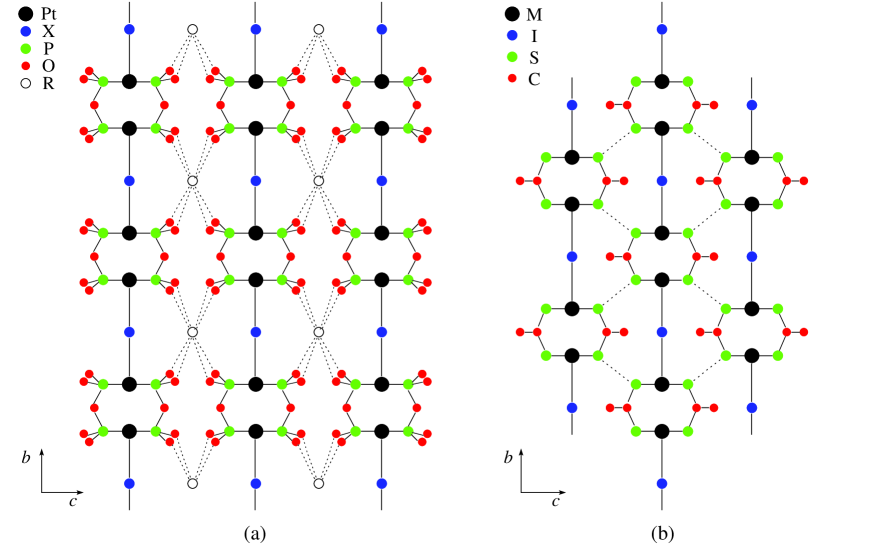
FIG. 1.: Crystal structures of the pop complexes $R_{4}$[Pt₂(pop)${}_{4}X$]$\cdot$$n$H₂O (a) and the dta complexes $M_{2}$(dta)₄I (b) in the projection of the $bc$ plane, where hydrogen atoms are omitted. The dotted lines represent hydrogen bonds in (a), while they correspond to van der Waals contacts in (b).

In recent years, binuclear metal analogs ($M\!M\!X$ chains) have made our argument more and more exciting. They comprise two families: $R_{4}$[Pt₂(pop)${}_{4}X$]$\cdot$$n$H₂O ($X=\mbox{Cl},\mbox{Br},\mbox{I}$; $R=\mbox{Li},\mbox{K},\mbox{Cs},\cdots$; $\mbox{pop}=\mbox{diphosphonate}=\mbox{P}_{2}\mbox{O}_{5}\mbox{H}_{2}^{\,2-}$) [10, 11] [Fig. 1(a)] and $M_{2}$(dta)₄I ($M=\mbox{Pt},\mbox{Ni}$; $\mbox{dta}=\mbox{dithioacetate}=\mbox{CH}_{3}\mbox{CS}_{2}^{\,-}$) [12, 13] [Fig. 1(b)]. The pop complexes are in general semiconductors with charge-density-wave ground states of the conventional type [14, 15] [Fig. 2(a)]. However, due to the small Peierls gaps, their ground states can be tuned by replacing the halogens and/or counter ions [16]. Such tuning of the electronic state is feasible also by pressure [17]. On the other hand, the dta-family platinum complex, Pt₂(dta)₄I, exhibits metallic conduction at room temperature [18], which has never been realized in conventional $M\!X$ compounds. With decreasing temperature, there occurs a metal-semiconductor transition at $300$ K and further transition to a novel charge-ordering mode [Fig. 2(b)] follows around $80$ K [19].

The exciting observations have stimulated theoretical research. Carrying out quantum-chemical band calculations, Borshch et al. [20] attributed the novel valence distribution in Pt₂(dta)₄I to its structural distortion. Kuwabara and Yonemitsu [21] more extensively investigated the charge ordering and lattice modulation using various numerical tools. The author [22] also studied the ground-state properties with particular emphasis on the contrast between the dta and pop complexes. Quantum, thermal, and pressure-induced phase transitions were theoretically demonstrated [23, 24] so as to interpret the observations, while the optical conductivity was calculated [25] in an attempt to evaluate the hopping amplitudes and Coulomb interactions.

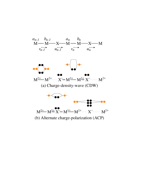
FIG. 2.: Schematic representation of the two distinct ground states of $M\!M\!X$ chains [19]: (a) Charge-density-wave (CDW) state whose $X$ sublattice is dimerized; (b) Alternate charge-polarization (ACP) state whose $M_{2}$ sublattice is dimerized.

Now we are led to take a step toward the excited states. Solitonic excitations are expected of doubly (or multiply in general) degenerate charge-density-wave systems. Ichinose [26] introduced the idea of domain walls into $M\!X$ chains and Onodera [27] developed the argument pointing out some similarities between $M\!X$ chains and the trans isomer of polyacetylene in the weak-coupling region. Baeriswyl and Bishop [28] extended the calculation to polaronic states laying emphasis on the strong-coupling region. Optical absorption spectra due to solitons and polarons [2, 29] and their relaxation process [30, 31] in $M\!X$ chains were extensively investigated. Although photoexperiments on $M\!M\!X$ chains [32] are still in their early stage, the optical excitations must be a coming potential subject. Making full use of a simple but relevant electron-phonon model, we give a detailed description of intrinsic defects in $M\!M\!X$ chains. Numerical calculations, together with an analytic argument in the weak-coupling region, reveal that $M\!M\!X$ chains still exhibit a striking analogy with trans-polyacetylene in their excitation mechanism.

FIG. 3.: The $\alpha$-versus-$\beta$ ground-state phase diagrams at various values of $t_{\rm MXM}$.

II Model Hamiltonian

We employ the $\frac{3}{4}$-filled one-dimensional single-band two-orbital electron-phonon model:

$${\cal H}=-t_{\rm MM}\sum_{n,s}(a_{n,s}^{\dagger}b_{n,s}+b_{n,s}^{\dagger}a_{n,s})$$ (1)

$$\quad-\sum_{n,s}\bigl{[}t_{\rm MXM}-\alpha(l_{n+1}^{\rm(a)}+l_{n}^{\rm(b)})\bigr{]}(a_{n+1,s}^{\dagger}b_{n,s}+b_{n,s}^{\dagger}a_{n+1,s})$$ (2)

$$\quad-\beta\sum_{n,s}(l_{n}^{\rm(a)}a_{n,s}^{\dagger}a_{n,s}+l_{n}^{\rm(b)}b_{n,s}^{\dagger}b_{n,s})$$ (3)

$$\quad+\frac{K_{\rm MX}}{2}\sum_{n}\bigl{[}(l_{n}^{\rm(a)})^{2}+(l_{n}^{\rm(b)})^{2}\bigr{]}\,,$$ (4)

where $a_{n,s}^{\dagger}$ and $b_{n,s}^{\dagger}$ are the creation operators of an electron with spin $s=\pm$ (up and down) for the $M$ $d_{z^{2}}$ orbitals in the $n$th $M\!M\!X$ unit. $t_{\rm MM}$ and $t_{\rm MXM}$ describe the intradimer and interdimer electron hoppings, respectively. $\alpha$ and $\beta$ are the intersite and intrasite electron-phonon coupling constants, respectively, with $K_{\rm MX}$ being the metal-halogen spring constant. $l_{n}^{\rm(a)}=v_{n}-u_{n-1}$ and $l_{n}^{\rm(b)}=u_{n}-v_{n}$ with $u_{n}$ and $v_{n}$ being, respectively, the chain-direction displacements of the halogen and metal dimer in the $n$th $M\!M\!X$ unit from their equilibrium position. We assume, based on the thus-far reported experimental observations, that every $M_{2}$ moiety is not deformed. The notation is further explained in Fig. 2. We set $t_{\rm MM}$ and $K$ both equal to unity in the following.

The Hamiltonian (4) convincingly describes the two distinct ground states of $M\!M\!X$ chains, which are schematically shown in Fig. 2. The CDW and ACP states are characterized by the alternating on-site electron affinities and interdimer transfer energies, respectively. Orbital hybridization mainly stays within each $M_{2}$ moiety in the valence-trapped CDW state, while it essentially extends over neighboring $M_{2}$ moieties in the valence-delocalized ACP state. Therefore, the CDW state is more stabilized by increasing $\beta$ and $t_{\rm MM}$, whereas the ACP state by increasing $\alpha$ and $t_{\rm MXM}$. The $M_{2}$ moieties are tightly locked together in the pop complexes due to the hydrogen bonds between the ligands and counter cations, while they are rather movable in the dta complexes owing to the neutral chain structure. Thus a significantly larger $\alpha$ is expected for the dta complexes. In this context, Fig. 3 is well consistent with experimental observations; (NH₄)₄[Pt₂(pop)₄Cl] exhibits a ground state of the CDW type [15], while Pt₂(dta)₄I displays that of the ACP type [19]. In the weak-coupling region, $v_{n}=0$ in CDW, whereas $u_{n}=0$ in ACP. With increasing coupling constants, their arise mixed states with $u_{n}\neq 0$ and $v_{n}\neq 0$ [28, 33, 34]. We note that the present CDW and ACP are characterized as the lattice configurations $l_{n}^{(a)}=l_{n}^{(b)}$ and $l_{n}^{(a)}=-l_{n}^{(b)}$, respectively, regardless of each displacement $u_{n}$ and $v_{n}$.

III Results and Discussion

A Variational Treatment

We consider local excitations from these ground states. Under the constraint of the total chain length being unchanged, trial wave functions may be introduced as

$$l_{n}^{\rm(a)}=\sigma l_{n}^{\rm(b)}=(-1)^{n}l_{0}{\rm tanh}\bigl{[}(na-x_{0})/\xi\bigr{]}\,,$$ (5)

for solitons [35] and as

$$l_{n}^{\rm(a)}=\sigma l_{n}^{\rm(b)}=(-1)^{n}l_{0}\bigl{\{}1-{\rm tanh}(2\kappa d)$$ (6)

$$\quad\times\bigl{[}{\rm tanh}\kappa(na-x_{0}+d)-{\rm tanh}\kappa(na-x_{0}-d)\bigr{]}\bigr{\}}\,,$$ (7)

for polarons [36, 37], where $\sigma$ takes $+$ and $-$ on the CDW and ACP backgrounds, respectively, $a$ is the lattice constant, and $l_{0}$ is the metal-halogen bond-length change in the ground state. $x_{0}$ indicates the defect center in both functions, while $\xi$ and $\kappa^{-1}{\rm tanh}(2\kappa d)$ describe the spatial extents of solitons and polarons, respectively, all of which are variationally determined. Since we impose the periodic boundary condition on the Hamiltonian, the soliton solutions assume that the number of the original unit cells, $N$, should be odd, whereas the polaron solutions assume that $N$ should be even. We set $N$ equal to $201$ or $200$, either of which is much larger than any defect extent in our calculation. Defect energies are degenerate with respect to their spin, but it is not the case with their charge due to the broken electron-hole symmetry. When we compare the defects on the CDW and ACP backgrounds, we calculate them near the phase boundary so as to illuminate their essential differences. Taking the structural analyses [10, 11, 12] into consideration, we set $t_{\rm MM}=2t_{\rm MXM}$.

B Spatial Configuration and Energy Structure

We show in Fig. 5 the spatial configurations of the optimum defect solutions. Spin and charge are separate entities in the solitonic excitations, while the polaronic excitations exhibit the conventional spin-charge characteristics. Neutral solitons S⁰ and polarons P^± convey net spin densities $\pm\frac{1}{2}$, whereas no spin density accompanies charged solitons S^±. Their formation energies do not depend on their locations in the weak-coupling region, but the degeneracy is lifted with increasing coupling strength (Table I). As the Peierls gap increases, defects generally possess increasing energies and decreasing extents, and end up with immobile entities.

In order to investigate their electronic structures in more detail, we decompose the electron densities $a_{n}$ and $b_{n}$ into alternating ($\widetilde{a}_{n}$, $\widetilde{b}_{n}$) and net (nonalternating) ($\overline{a}_{n}$, $\overline{b}_{n}$) components as

$$\left.\begin{array}[]{ll}a_{n}=\overline{a}_{n}+\widetilde{a}_{n}\,;&\overline{a}_{n}=\frac{\displaystyle 1}{\displaystyle 4}(a_{n-1}+2a_{n}+a_{n+1})\,,\\ b_{n}=\overline{b}_{n}+\widetilde{b}_{n}\,;&\overline{b}_{n}=\frac{\displaystyle 1}{\displaystyle 4}(b_{n-1}+2b_{n}+b_{n+1})\,,\\ \end{array}\right.$$ (8)

and show them for positively charged solitons S⁺ in Fig. 5. Now we can easily find out the positive charges accompanying the defects. One of the most interesting and important features of local excitations of this kind is their interfacial character. Let us define further the CDW and ACP order parameters using the alternating components as

$$\left.\begin{array}[]{lll}O_{n}^{\rm CDW}&=&\frac{\displaystyle(-1)^{n}}{\displaystyle 2}\left(\widetilde{a}_{n}+\widetilde{b}_{n}\right)\,,\\ O_{n}^{\rm ACP}&=&\frac{\displaystyle(-1)^{n}}{\displaystyle 2}\left(\widetilde{a}_{n}+\widetilde{b}_{n-1}\right)\,,\\ \end{array}\right.$$ (9)

which detect oscillations of the CDW and ACP types, respectively, and are also plotted in Fig. 5. We learn that the CDW soliton reduces the CDW amplitude and induces the ACP amplitude instead in its center, while vice versa for the ACP solion. Their trajectories are expressed as ${\rm CDW}\rightarrow{\rm ACP}\rightarrow\overline{\rm CDW}$ and ${\rm ACP}\rightarrow\overline{\rm CDW}\rightarrow\overline{\rm ACP}$, where $\overline{\rm A}$ denotes the antiphase counterpart for the state A. Neutral solitons and polarons exhibit different types of interface, where certain kinds of spin-density-wave oscillation blend into CDW or ACP. Due to their mixed nature, solitons and polarons could be divided into more elementary defects in the vicinity of the phase boundaries.

Density of states for solitons and polarons are shown in Fig. 6. The four bands coming from the CDW background are, from the bottom to the top, largely made up of the bonding combination $\phi_{+}$ of binuclear Pt²⁺-Pt²⁺ units, that of Pt³⁺-Pt³⁺ units, the antibonding combination $\phi_{-}$ of Pt²⁺-Pt²⁺ units, and that of Pt³⁺-Pt³⁺ units. On the other hand, the major components of the four bands coming from the ACP background are the $\phi_{+}$ orbitals of interdimer Pt²⁺-X^--Pt²⁺ units, the $\phi_{-}$ orbitals of Pt²⁺-X^--Pt²⁺ units, the $\phi_{+}$ orbitals of Pt³⁺-X^--Pt³⁺ units, and the $\phi_{-}$ orbitals of Pt³⁺-X^--Pt³⁺ units. Therefore, increasing $\beta$ splits both $\sigma$ and $\sigma^{*}$ orbitals in the CDW state, while in the ACP state the splitting between $\sigma$ and $\sigma^{*}$ orbitals is stressed as an effect of increasing $\beta$.

  

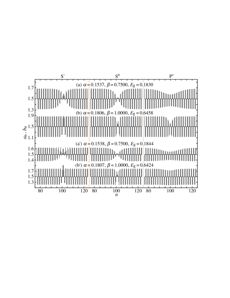
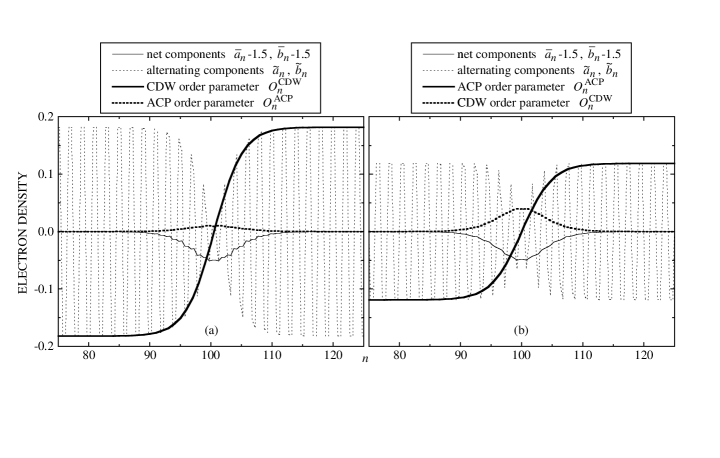
FIG. 4.: Spatial configurations of negatively charged solitons S^-, neutral solitons S⁰, and positively charged polarons P⁺ in the CDW (a and b) and ACP (a^′ and b^′) states, where quantum averages of the local electron densities, $\sum_{s}\langle a_{n,s}^{\dagger}a_{n,s}\rangle\equiv a_{n}$ and $\sum_{s}\langle b_{n,s}^{\dagger}b_{n,s}\rangle\equiv b_{n}$, are measured in comparison with the average occupancy.

 

FIG. 5.: Spatial configurations of positively charged solitons S⁺ on the CDW (a; $\alpha=0.1537$, $\beta=0.7500$) and ACP (b; $\alpha=0.1538$, $\beta=0.7500$) backgrounds, where their alternating and net components (see in the text) are separately shown and the CDW and ACP order parameters (see in the text) are also plotted.

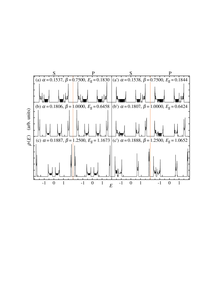
FIG. 6.: Density of states $\rho(E)$ for the optimum soliton and polaron solutions on the CDW ($\mbox{a},\mbox{b},\mbox{c}$) and ACP ($\mbox{a}^{\prime},\mbox{b}^{\prime},\mbox{c}^{\prime}$) backgrounds.

The soliton solutions commonly exhibit an additional level within the gap, whereas the polaron ones are accompanied by a couple of intragap levels. These levels are all found to be localized around the defect center. The level structures in the weak-coupling region suggest some similarities between small-gap $M\!M\!X$ chains and trans-polyacetylene. However, in contrast with the case of polyacetylene [35, 37], the level structure which is symmetric with respect to the middle of the gap greaks down with increasing electron-phonon interactions due to the lack of electron-hole symmetry. Besides the intragap levels, there appear a few related levels which are also localized around the defect center.

C Scaling Properties

In order to illuminate the scaling properties of the solitons and polarons in more detail, we plot in Fig. 7 their characteristic lengths $\xi$ and $\kappa^{-1}{\rm tanh}(2\kappa d)$ as functions of the band gap $E_{\rm g}$. Although we have calculated them with varying $\alpha$, $\beta$, and $x_{0}$, they are uniquely scaled by $E_{\rm g}$ in the weak-coupling region as

$$\xi/a\sim 0.95/E_{\rm g}^{0.98}\,,\ \ {\rm tanh}(2\kappa d)/\kappa a\sim 0.88/E_{\rm g}^{1.03}\,,$$ (10)

where the second decimal place varies with the data set taken into the fitting. It is convincing that such scaling laws break down as the defect extents come close to the length scale $a$. The formation energies are also scaled by the gap, as is shown in Fig. 8. In the weak-coupling region, the soliton and polaron energies are both degenerate with respect to their spin and location, and exhibit scaling formulae

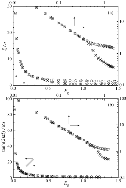
FIG. 7.: The optimized extents of the solitons (a) and polarons (b) as functions of the band gap $E_{\rm g}$ in linear and logarithmic scales under various values of $\alpha$ and $\beta$, where $\circ$ and $\times$ correspond to the highest- and lowest-energy locations $x_{0}$, respectively.

FIG. 8.: The soliton and polaron formation energies averaged over $x_{0}$ as functions of the band gap $E_{\rm g}$. The negatively (positively) charged solitons and polarons possess more (less) than three-quarter-filled electron bands and therefore their formation energies can not be defined in themselves. As for charged excitations, $E_{\rm S}$ ($E_{\rm P}$) is further averaged over S⁺ (P⁺) and S^- (P^-).

$$E_{\rm S}\sim 0.33E_{\rm g}\,,\ \ E_{\rm P}\sim 0.46E_{\rm g}\,.$$ (11)

With increasing gap, the degeneracy is lifted, where the CDW solitons have lower energies than their ACP counterparts at a given $E_{\rm g}$, while vice versa for polarons. Now that we have obtained the numerical observations (11), we should be reminded of the defect states in trans-polyacetylene and a rigorous approach [37, 38] to them.

Su, Schrieffer, and Heeger (SSH) [35] pioneeringly presented a theoretical study on the soliton excitations in polyacetylene. Although they employed a simple electron-phonon model, essential features of solitons such as the midgap localized energy level and the small effective mass were successfully interpreted. Takayama, Lin-Liu, and Maki (TLM) [38] mapped the SSH model onto a continuous line and obtained a rigorous soliton solution with the formation energy $E_{\rm S}=E_{\rm g}/\pi$. A polaron solution [36, 37] was also found within the same scheme and its formation energy was revealed as $E_{\rm P}=\sqrt{2}E_{\rm g}/\pi$. Our numerical estimates (11), which are very close to the TLM findings, suggest that $M\!M\!X$ chains still have an analogy with polyacetylene. Inquiring the continuum-model description of $M\!M\!X$ chains, we try to understand the numerical calculations.

The continuum version of the present model (4) should be constructed from the primary $d_{\sigma^{*}}$ conduction band under no dimerization of the system. Without any electron-phonon coupling, the Hamiltonian (4) can be expressed as

$$\lim_{\alpha,\beta\rightarrow 0}{\cal H}=\sum_{k,s}\left(\varepsilon_{k}^{+}A_{k,s}^{\dagger}A_{k,s}+\varepsilon_{k}^{-}B_{k,s}^{\dagger}B_{k,s}\right)\,,$$ (12)

where

$$\varepsilon_{k}^{\pm}=\pm\sqrt{t_{\rm MM}^{2}+t_{\rm MXM}^{2}+2t_{\rm MM}t_{\rm MXM}{\rm cos}ka}\,,$$ (13)

$$\left.\begin{array}[]{lll}A_{k,s}&=&\frac{\displaystyle 1}{\displaystyle\sqrt{2}}\left({\rm e}^{{\rm i}\theta/2}a_{k,s}+{\rm e}^{{\rm-i}\theta/2}b_{k,s}\right)\,,\\ B_{k,s}&=&\frac{\displaystyle 1}{\displaystyle\sqrt{2}}\left({\rm e}^{{\rm i}\theta/2}a_{k,s}-{\rm e}^{-{\rm i}\theta/2}b_{k,s}\right)\,,\\ \end{array}\right.$$ (14)

with $a_{k,s}$ ($b_{k,s}$) being the Fourier transform of $a_{n,s}$ ($b_{n,s}$) and

$${\rm e}^{{\rm i}\theta}=-\frac{t_{\rm MM}+t_{\rm MXM}{\rm e}^{{\rm i}ka}}{\sqrt{t_{\rm MM}^{2}+t_{\rm MXM}^{2}+2t_{\rm MM}t_{\rm MXM}{\rm cos}ka}}\,.$$ (15)

As far as we restrict our interest to the low-lying excitations, we may discard the irrelevant $d_{\sigma}$ band, which is here described by the dispersion relation $\varepsilon_{k}^{-}$, and linearize the relevant dispersion $\varepsilon_{k}^{+}$ at the two Fermi points. Taking account of the electron-phonon coupling within this scheme and assuming the CDW and ACP backgrounds, we obtain two effective Hamiltonians in the coordinate representation:

$${\cal H}_{\rm eff}^{\rm CDW}=t_{\rm eff}\sum_{n,s}\left[1-\frac{{\mit\Delta}(na)}{t_{\rm MM}}\right]\left(A_{n,s}^{\dagger}A_{n+1,s}+{\rm H.c.}\right)$$ (16)

$$\ +\frac{2t_{\rm eff}}{t_{\rm MXM}}\sum_{n,s}{\mit\Delta}(na)A_{n,s}^{\dagger}A_{n,s}+\frac{K_{\rm MX}}{4\beta_{\rm eff}^{2}}\sum_{n}{\mit\Delta}(na)^{2}\,,$$ (17)

$${\cal H}_{\rm eff}^{\rm ACP}=t_{\rm eff}\sum_{n,s}\left[1-\frac{{\mit\Delta}(na)}{t_{\rm MXM}}\right]\left(A_{n,s}^{\dagger}A_{n+1,s}+{\rm H.c.}\right)$$ (18)

$$\ +\frac{2t_{\rm eff}}{t_{\rm MM}}\sum_{n,s}{\mit\Delta}(na)A_{n,s}^{\dagger}A_{n,s}+\frac{K_{\rm MX}}{16\alpha_{\rm eff}^{2}}\sum_{n}{\mit\Delta}(na)^{2}\,,$$ (19)

where

$$t_{\rm eff}=\frac{t_{\rm MM}t_{\rm MXM}}{2\sqrt{t_{\rm MM}^{2}+t_{\rm MXM}^{2}}}\,,$$ (20)

$$\alpha_{\rm eff}=\frac{1}{2}\left(\alpha+\frac{t_{\rm eff}}{t_{\rm MM}}\beta\right)\,,\ \ \beta_{\rm eff}=\frac{t_{\rm eff}}{t_{\rm MXM}}\beta\,,$$ (21)

$${\mit\Delta}(na)=\left\{\begin{array}[]{l}2\beta_{\rm eff}(-1)^{n}(u_{n}-v_{n})\ \ \ {\rm for}\ {\cal H}_{\rm eff}^{\rm CDW}\,,\\ 4\alpha_{\rm eff}(-1)^{n}(u_{n}-v_{n})\ \ \ {\rm for}\ {\cal H}_{\rm eff}^{\rm ACP}\,.\\ \end{array}\right.$$ (22)

In accordance with the slowly-varying gap parameter ${\mit\Delta}(na)$, we introduce operators

$$\left.\begin{array}[]{lll}\psi_{s}^{\rm(r)}(na)&=&\frac{\displaystyle 1}{\displaystyle\sqrt{L}}{\displaystyle\sum_{k}}{\rm e}^{{\rm i}kna}A_{k_{\rm F}+k,s}\,,\\ \psi_{s}^{\rm(l)}(na)&=&\frac{\displaystyle-{\rm i}}{\displaystyle\sqrt{L}}{\displaystyle\sum_{k}}{\rm e}^{{\rm i}kna}A_{-k_{\rm F}+k,s}\,,\\ \end{array}\right.$$ (23)

for right- and left-moving electrons, respectively, where $L=Na$, $k_{\rm F}=\pi/2a$ and $-\pi/2a<k\leq\pi/2a$. Now, summing out fast-varying components and taking the $a\rightarrow 0$ limit, we reach the relevant continuum models

$${\cal H}_{\rm eff}^{\rm CDW}=\int\frac{{\mit\Delta}(x)^{2}}{2\pi\hbar v_{\rm F}\lambda}{\rm d}x+\sum_{s}\int{\mit\Phi}_{s}^{\dagger}(x)\biggl{[}{\rm i}\hbar v_{\rm F}\sigma_{z}\frac{{\rm d}}{{\rm d}x}$$ (24)

$$\quad-2{\mit\Delta}(x)t_{\rm eff}\left(\frac{\sigma_{x}}{t_{\rm MM}}+\frac{\sigma_{y}}{t_{\rm MXM}}\right)\biggr{]}{\mit\Phi}_{s}(x){\rm d}x\,,$$ (25)

$${\cal H}_{\rm eff}^{\rm ACP}=\int\frac{{\mit\Delta}(x)^{2}}{2\pi\hbar v_{\rm F}\lambda}{\rm d}x+\sum_{s}\int{\mit\Phi}_{s}^{\dagger}(x)\biggl{[}{\rm i}\hbar v_{\rm F}\sigma_{z}\frac{{\rm d}}{{\rm d}x}$$ (26)

$$\quad-2{\mit\Delta}(x)t_{\rm eff}\left(\frac{\sigma_{x}}{t_{\rm MXM}}+\frac{\sigma_{y}}{t_{\rm MM}}\right)\biggr{]}{\mit\Phi}_{s}(x){\rm d}x\,,$$ (27)

where we have employed the Pauli matrices $(\sigma_{x},\sigma_{y},\sigma_{z})$ and a spinor notation ${\mit\Phi}_{s}^{\dagger}(x)=(\psi_{s}^{\rm(r)}(x)^{*},\psi_{s}^{\rm(l)}(x)^{*})$, defining the Fermi velocity $v_{\rm F}$ and the dimensionless coupling constant $\lambda$ as

$$\hbar v_{\rm F}=2at_{\rm eff}\,,$$ (28)

$$\lambda=\left\{\begin{array}[]{l}\beta_{\rm eff}^{2}/\pi t_{\rm eff}K_{\rm MX}\ \ \ {\rm for}\ {\cal H}_{\rm eff}^{\rm CDW}\,,\\ 4\alpha_{\rm eff}^{2}/\pi t_{\rm eff}K_{\rm MX}\ \ \ {\rm for}\ {\cal H}_{\rm eff}^{\rm ACP}\,.\\ \end{array}\right.$$ (29)

Interestingly, when we rotate the spinor wave function around the $z$ axis by the angle

$$\varphi=\left\{\begin{array}[]{l}{\rm arctan}(t_{\rm MM}/t_{\rm MXM})\ \ \ {\rm for}\ {\cal H}_{\rm eff}^{\rm CDW}\,,\\ {\rm arctan}(t_{\rm MXM}/t_{\rm MM})\ \ \ {\rm for}\ {\cal H}_{\rm eff}^{\rm ACP}\,,\\ \end{array}\right.$$ (30)

both Hamiltonians (25) and (27) turn into the same expression

$${\cal H}_{\rm TLM}=\int\frac{{\mit\Delta}(x)^{2}}{2\pi\hbar v_{\rm F}\lambda}{\rm d}x+\sum_{s}\int{\mit\Phi}_{s}^{\dagger}(x)$$ (31)

$$\quad\times\left[-{\rm i}\hbar v_{\rm F}\sigma_{z}\frac{{\rm d}}{{\rm d}x}+{\mit\Delta}(x)\sigma_{x}\right]{\mit\Phi}_{s}(x){\rm d}x\,,$$ (32)

which is nothing but the TLM continuum model. We know that the Hamiltonian (32) possesses exact solitonic [38, 39] and polaronic [36, 37] solutions

$${\mit\Delta}(x)={\mit\Delta}_{0}{\rm tanh}(x/\xi)\,,$$ (33)

$${\mit\Delta}(x)={\mit\Delta}_{0}-\hbar v_{\rm F}\kappa$$ (34)

$$\quad\times\bigl{[}{\rm tanh}\kappa(x+d)-{\rm tanh}\kappa(x-d)\bigr{]}\,,$$ (35)

with their characteristic scaling relations

$$\xi=\hbar v_{\rm F}/{\mit\Delta}_{0}\,,\ \ E_{\rm S}=2{\mit\Delta}_{0}/\pi\,,$$ (36)

$${\rm tanh}(2\kappa d)/\kappa=\hbar v_{\rm F}/{\mit\Delta}_{0}\,,\ \ E_{\rm P}=2\sqrt{2}{\mit\Delta}_{0}/\pi\,.$$ (37)

Considering Eqs. (20) and (28) together with the relation $2{\mit\Delta}_{0}=E_{\rm g}$, we are fully convinced of the present numerical findings (10) and (11).

FIG. 9.: The soliton and polaron masses as functions of the band gap $E_{\rm g}$ in the unit of the electron mass $m_{\rm e}$. All the excitations are almost degenerate with respect to their spin, charge, and location in the weak-coupling region, but the degeneracy is lifted with increasing gap. As for charged defects, we have simply plotted the masses of negatively charged ones, because those of positively charged ones are less convergent in the strong-coupling region, much more rapidly increasing with gap outside the weak-coupling region.

D Effective Mass

The continuum-model analysis has revealed that the defect extents should be given by $2a/\sqrt{5}E_{\rm g}$ in the weak-coupling limit under the present parametrization. According to the numerical observations (10), this scaling law better holds for polarons than for solitons. This may be because polarons have wider extents than solitons at a given gap. When we consider moving defects, such an idea is quite suggestive. Let us calculate the effective masses of solitons and polarons.

Moving the defect center as $x_{0}=vt$ in Eqs. (5) and (7) and neglecting any change in the defect shape, which must be of order $v^{2}$ due to the time-reversal symmetry and therefore does not contribute to the defect mass $M_{\rm defect}$ for small $v$, we find

$$\frac{1}{2}M_{\rm defect}v^{2}=\frac{1}{2}M\sum_{n}(\dot{l}_{n}^{\rm(a)})^{2}\,,$$ (38)

where $M$ corresponds to the mass of a halogen or bimetal complex according as the ground state is CDW or ACP. Assuming $n$ to be sufficiently large under the periodic boundary condition, the summation in Eq. (38) can explicitly be taken and ends up with

$$M_{\rm S}=\frac{4Ma}{3\xi}\left(\frac{l_{0}}{a}\right)^{2}\,,$$ (39)

$$M_{\rm P}=\frac{8}{3}M\kappa a\left(\frac{l_{0}}{a}\right)^{2}{\rm tanh}^{2}(2\kappa d)$$ (40)

$$\quad\times\biggl{[}1-12\frac{2\kappa d+1+(2\kappa d-1){\rm e}^{4\kappa d}}{{\rm e}^{12\kappa d}-3{\rm e}^{8\kappa d}+3{\rm e}^{8\kappa d}-1}\biggr{]}\,,$$ (41)

for solitons and polarons, respectively. Further calculation is performed for two well-studied $M\!M\!X$-chain materials K₄[Pt₂(pop)₄Br]$\cdot$$3$H₂O [10, 14, 17, 40, 41] with $a=8.139$ Å[14] and Pt₂(dta)₄I [12, 18, 19, 42, 43] with $a=8.633$ Å[12]. Their ground states were assigned to CDW and ACP, respectively, and therefore they give $M=145611m_{\rm e}$ and $M=1375629m_{\rm e}$, respectively, where $m_{\rm e}$ is the electron mass. We show in Fig. 9 the thus calculated soliton and polaron masses, where the optimum values of $\xi$, $\kappa$, and $d$ have been averaged over $x_{0}$. For $E_{\rm g}\gtrsim 0.4$, any defect has to overcome site-dependent energy barriers in its motion and thus the present calculations are just for reference.

In comparison with the formation energy which describes a static defect and is generically given for both types of ground state in the weak-coupling region, the effective mass of a moving defect varies according to the background charge ordering. Defects on the ACP background generally look more massive than their CDW counterparts. However, the difference should rather be attributed to the material-dependent crystalline structure than be recognized as a result of intrinsic defect features. CDW is accompanied by the halogen-sublattice dimerization, while ACP by the metal-sublattice dimerization. Larger defect masses on the ACP background reflect the mass of the diplatinum complex Pt₂(CH₃CS₂)₄ which is about ten times as heavy as the halogen atom Br.

On the other hand, the polaron mass turns out intrinsically smaller than the soliton mass. We have indeed found in Fig. 5 that the polarons are more spatially extended than the solitons at a given gap. The energy gap at least amounts to $0.75$ eV [44] in conventional $M\!X$-chain materials. Metal binucleation strikingly reduces the gap, for example, to $0.08$ eV for K₄[Pt₂(pop)₄Br]$\cdot$$3$H₂O [14] and $0.05$ eV for Pt₂(dta)₄I [12]. Correspondingly, Pt₂(dta)₄I exhibits a high electrical conductivity $13$ $\Omega^{-1}\mbox{cm}^{-1}$ [19], which is about $10^{9}$ times larger than that of a typical $M\!X$ compound. Though we have no information on $t_{\rm MM}$, previous estimates of $t_{\rm MXM}$ for $M\!X$ compounds [45, 46], together with the structural analyses [10, 11, 12], imply that $t_{\rm MM}=1\sim 2$ eV for $M\!M\!X$ compounds. Then we are allowed to estimate that $0.1m_{\rm e}\lesssim M_{\rm S}\lesssim 2m_{\rm e}$ and $0.05m_{\rm e}\lesssim M_{\rm P}\lesssim m_{\rm e}$ for K₄[Pt₂(pop)₄Br]$\cdot$$3$H₂O, while $0.3m_{\rm e}\lesssim M_{\rm S}\lesssim 3m_{\rm e}$ and $0.1m_{\rm e}\lesssim M_{\rm P}\lesssim m_{\rm e}$ for Pt₂(dta)₄I. In any case, the $M\!M\!X$-solitons are a few times as heavy as the $M\!M\!X$-polarons but still much lighter than the $M\!X$-solitons of $M_{\rm S}\gtrsim 100m_{\rm e}$ [27]. There is a similar observation in trans-polyacetylene as well. The TLM-model analysis of polyacetylene gives $M_{\rm S}\simeq 3m_{\rm e}$ [47] and $M_{\rm P}\simeq m_{\rm e}$ [37]. Such small masses should be quite significant in dynamics involving solitons and polarons. From the energetical point of view, we have learnt that $E_{\rm P}<2E_{\rm S}<2E_{\rm P}$. We can not well distinguish charged solitons from neutral ones within the electron-phonon model, but we find, taking account of electron-electron correlation, that $E_{{\rm S}^{0}}<E_{{\rm S}^{\pm}}$ [48]. Hence there may be a relaxation of photogenerated polaron pairs $\mbox{P}^{+}+\mbox{P}^{-}\longrightarrow\mbox{S}^{0}+\bar{\mbox{S}}^{0}$ and a recombination of doping-induced or chemical-defect-associated solitons $\mbox{S}^{\pm}+\bar{\mbox{S}}^{0}\longrightarrow\mbox{P}^{\pm}$. In $M\!X$ compounds, photogeneration of solitons and polarons have indeed been observed and they exhibit a varied relaxation process within a few hundred psec [6, 8, 9]. $M\!M\!X$ chains with less massive defects may really exhibit picosecond dynamics.

IV Concluding Remarks

We have investigated the local excitations corresponding to topological solitons and polarons in halogen-bridged diplatinum chains in terms of a coupled electron-phonon model. Although the solitons have lower excitation energies than the polarons, the effective masses of the solitons are larger than those of polarons. Their high mobility is promised in $M\!M\!X$ chains with small energy gaps up to $\sim 0.1$ eV, where all the defects are at most a few times as massive as an electron.

There is an analogy between the defect states in $M\!M\!X$ chains and those in trans-polyacetylene in spite of many contrasts between these systems such as $d$ and $\pi$ electrons, binuclear and mononuclear assemblies, and intrasite and intersite electron-phonon couplings. Then we are all the more eager to encourage optical measurements and doping of $M\!M\!X$ chains, where the electronic gap is suitably small, chemical tuning of the electronic state is widely possible, and the single crystals are readily available.

TABLE I.: The lowest- and highest-energy locations $x_{0}$ of $M\!M\!X$ solitons and polarons.

	CDW background		ACP background
	the lowest	the highest	the lowest	the highest
S-	$(2n-\frac{1}{2})a$	$(2n+\frac{1}{2})a$	$(2n+1)a$	$2na$
S+	$(2n+\frac{1}{2})a$	$(2n-\frac{1}{2})a$	$2na$	$(2n+1)a$
S0	$(2n-\frac{1}{2})a$	$(2n+\frac{1}{2})a$	$(2n+1)a$	$2na$
P-	$(2n+1)a$	$2na$	$(2n+\frac{1}{2})a$	$(2n-\frac{1}{2})a$
P+	$2na$	$(2n+1)a$	$(2n-\frac{1}{2})a$	$(2n+\frac{1}{2})a$