Fermionic description of spin-gap states of antiferromagnetic Heisenberg ladders
in a magnetic field

PACS numbers: 75.10.Jm, 75.60.Ej

Spin gaps$-$the energy gaps in magnetic excitation spectra$-$of low-dimensional Heisenberg antiferromagnets have been attracting considerable interest in recent years. This fascinating subject was initiated by Haldane [1], renewed at the opportunity of high-temperature superconductivity being discovered [2], and further developed via the synthesis of ladder materials [3, 4]. Dagotto, Riera and Scalapino [5] pioneeringly pointed out a possible electronic mechanism for the formation of spin gaps in two-leg ladders. Following investigations [6] revealed that assembling chains into ladders, the crossover between one and two dimensions is far from smooth$-$Heisenberg ladders with an even number of legs have a spin gap, while those with an odd number of legs have no gaps.

Spin ladders in a magnetic field provide further interesting topics. Their ground-state magnetization curves have extensively been studied [7, 8, 9, 10] in an attempt to find quantized plateaux. Spin-$S$ $L$-leg Heisenberg ladders

$${\cal H}=\sum_{n=1}^{N}\left(J\sum_{l=1}^{L}\mbox{\boldmath$S$}_{n,l}\cdot\mbox{\boldmath$S$}_{n+1,l}+J^{\prime}\sum_{l=1}^{L-1}\mbox{\boldmath$S$}_{n,l}\cdot\mbox{\boldmath$S$}_{n,l+1}\right)\,,$$ (1)

may exhibit magnetization plateaux at $M/M_{\rm sat}=m/LS$ provided $LS-m\in\mbox{\boldmath Z}$ [7, 11, 12], where $M$ and $M_{\rm sat}$ are the magnetization and its saturated value, respectively. Since coupled-chain materials are likely to be systematically obtained in the case of spin $\frac{1}{2}$ [13], most of numerical efforts are being devoted to $S=\frac{1}{2}$ ladders. Then, without any bond polymerization, the most tractable system of our interest is the three-leg ladder. Lanczos diagonalization of finite systems [7], a series-expansion technique [8] and density-matrix renormalization-group calculations [10] are all in agreement to support the existence of the plateau at $M/M_{\rm sat}=1/3$ for strong interchain coupling $J^{\prime}\gtrsim J$. As for more-than-three-leg ladders, the existence of plateaux as well as their surviving region is still left to be verified.

Spin-$\frac{1}{2}$ two- and three-leg ladders are indeed realized in layer materials Sr_n-1Cu_n+1O_2n ($n=3,5,\cdots$) [4, 13], while four- and five-leg ones in La_4+4nCu_8+2nO_14+8n ($n=2,3,\cdots$) [14]. It is unfortunate that nevertheless large degrees of freedom prevent us from making numerical access to multi-leg ladders. In such circumstances, we propose a systematic approach to Heisenberg ladders in order to describe their spin-gap states in a field. Employing the Jordan-Wigner transformation on a unique path and then making a mean-field treatment of the fermionic Hamiltonian, we semiquantitatively visualize the appearance of plateaux and estimate the corresponding critical interactions $J^{\prime}_{\rm c}$ at an arbitrary number of legs, $L$.

It is along a snake-like path, $(n,l)=(1,1)\rightarrow(1,2)\rightarrow\cdots\rightarrow(1,L)\rightarrow(2,L)\rightarrow(2,L-1)\rightarrow\cdots\rightarrow(2,1)\rightarrow(3,1)\rightarrow\cdots$, that we define spinless fermions. This elaborately ordered path was first proposed by Dai and Su [15] and turned out to describe the spin gap as a function of $L$ much better than the naively ordered path [16], which is usually employed. When we introduce renumbered spin operators $\widetilde{\mbox{\boldmath$S$}}_{n,l}=\mbox{\boldmath$S$}_{n,l}$ ($\mbox{\boldmath$S$}_{n,L-l+1}$) for an odd (even) $n$, the spinless fermions are created as $c_{n,l}^{\dagger}=\widetilde{S}_{n,l}^{+}{\rm exp}[-{\rm i}\pi(\sum_{i=1}^{n-1}\sum_{j=1}^{L}\widetilde{S}_{i,j}^{+}\widetilde{S}_{i,j}^{-}+\sum_{j=1}^{l-1}\widetilde{S}_{n,j}^{+}\widetilde{S}_{n,j}^{-})]$. Making a standard mean-field treatment [15] of the fermionic Hamiltonian and assuming the spatial homogeneity $\langle\widetilde{S}_{n,l}^{z}\rangle=\langle c_{n,l}^{\dagger}c_{n,l}\rangle-1/2=M/LN$, we obtain

$${\cal H}=\frac{M}{LN}\sum_{k}\sum_{l=1}^{L}\Bigl{[}2J+(2-\delta_{l,1}-\delta_{l,L})J^{\prime}\Bigr{]}c_{k,l}^{\dagger}c_{k,l}$$ (2)

$$\qquad+\frac{J^{\prime}}{2}\sum_{k}\sum_{l=1}^{L-1}\left(c_{k,l}^{\dagger}c_{k,l+1}+c_{k,l+1}^{\dagger}c_{k,l}\right)$$ (3)

$$\qquad+\frac{J}{2}\sum_{k}\sum_{l=1}^{L}\Bigl{[}{\rm e}^{-{\rm i}\pi(L-l)(2M/LN+1)}{\rm e}^{-{\rm i}k}$$ (4)

$$\qquad\quad+{\rm e}^{{\rm i}\pi(l-1)(2M/LN+1)}{\rm e}^{{\rm i}k}\Bigr{]}c_{k,l}^{\dagger}c_{k,L-l+1}$$ (5)

$$\qquad-\Bigl{(}J+\frac{L-1}{L}J^{\prime}\Bigr{)}M\Bigl{(}1+\frac{M}{LN}\Bigr{)}\,,$$ (6)

where $c_{k,l}^{\dagger}=N^{-1/2}\sum_{n}{\rm e}^{-{\rm i}kn}c_{n,l}^{\dagger}$. The effective Hamiltonian (6), together with the Zeeman term $-H\sum_{k}\sum_{l=1}^{L}(c_{k,l}^{\dagger}c_{k,l}-1/2)$, is numerically diagonalized, adopting the open boundary condition along rungs, while taking the thermodynamic limit under the periodic boundary condition along legs.

In order to verify the reliability of the present approach, we plot in Fig. 2 the thus-obtained spin gaps ($H_{{\rm c}1}$) and saturation fields ($H_{{\rm c}2}$), the former of which are compared with highly precise numerical estimates [17], whereas the latter of which with the exact solutions $H_{{\rm c}2}=2J+J^{\prime}[1+\cos(\pi/L)]$. Although the present scheme somewhat overestimates $H_{{\rm c}1}$ with increasing $L$, it correctly tells whether the gap survives or not. As for $H_{{\rm c}2}$, the present calculation can be regarded as exact. We further show in Fig. 2 typical calculations of the ground-state magnetization. All the plateaux satisfying the criterion $L/2-M/N\in\mbox{\boldmath Z}$ indeed appear with increasing $J^{\prime}$. Mean-field approaches generally underestimate quantum fluctuations and therefore necessarily overestimate the magnetization. Allow us, however, to stress that the length of a plateau is still well describable in our treatment, which is essential to estimate the lower boundaries of the plateau-surviving region.

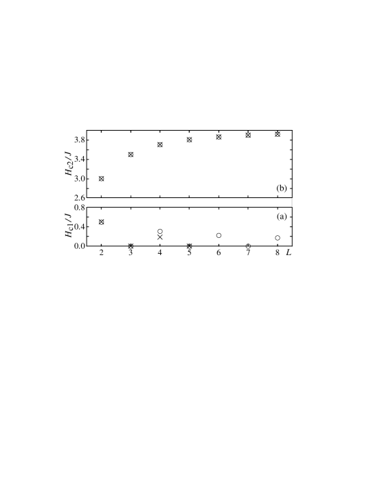
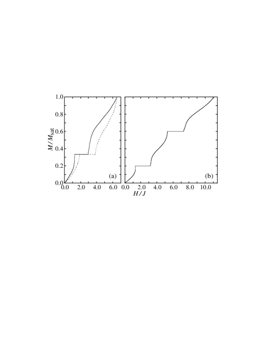
FIG. 1.: Spin gaps $H_{\rm c1}$ (a) and saturation fields $H_{\rm c2}$ (b) for the $L$-leg ladders with $J^{\prime}=J$, where the present culculations ($\circ$) are compared with density-matrix renormalization-group estimates [17] ($\times$) in (a) and with the exact values ($\times$) in (b).

FIG. 2.: Ground-state magnetization curves of the three- and five-leg ladders with $J^{\prime}=3J$ (a) and $J^{\prime}=5J$ (b), respectively. Numerical-diagonalization results [7] are also shown by a dotted line in (a).

Now we explore the main issue in Fig. 3. The critical value $J^{\prime}_{\rm c}=1.04\pm 0.01$ for $L=3$ is in good agreement with the previous estimate $J^{\prime}_{\rm c}\simeq J$ [8] obtained through the series expansion from the strong-rung-coupling limit $J/J^{\prime}\rightarrow 0$. $J^{\prime}_{\rm c}$ appears to increase with $L$, where even- and odd-$L$ ladders may form distinguishable series of their own. Here is a conclusive remark: Among possible nontrivial quantized magnetizations, $M/M_{\rm sat}=1-2/L,1-4/L,\cdots,2/L\,(1/L)$, the inner plateaux are easier to induce. The plateaux at the end-value magnetizations $M/M_{\rm sat}=1-2/L,2/L\,(1/L)$ are generally induced with larger $J^{\prime}$ than those at the inner-value magnetizations are. Practical observation of multi-plateau magnetization curves may less be feasible with increasing $L$. At the least, however, an available five-leg ladder material (La₂CuO₄)₃La₂Cu₄O₇ [14] encourages us to make theoretical explorations into the unique way from one- to two-dimensional antiferromagnets in a field. It is also important, further numerical verification of the plateau at $M/M_{\rm sat}=3/5$ more surviving than that at $M/M_{\rm sat}=1/5$ for $L=5$.

FIG. 3.: Critical interchain interaction to induce magnetization plateaux, $J^{\prime}_{\rm c}$, for the $L$-leg ladders, where the corresponding magnetization values $M/M_{\rm sat}$ are indicated beside symbols.

We are grateful to Prof. M. Takahasi for useful comments. This work was supported by the Japanese Ministry of Education, Science, Sports and Culture, and by the Sumitomo Foundation.

REFERENCES

- [1] F. D. M. Haldane: Phys. Rev. Lett. 50 (1983) 1153.
- [2] J. G. Bednorz and K. A. Müller: Z. Phys. B 64 (1986) 188.
- [3] D. C. Johnston, J. W. Johnson, D. P. Goshorn and A. J. Jacobson: Phys. Rev. B 35 (1987) 219.
- [4] Z. Hiroi, M. Azuma, M. Takano and Y. Bando: J. Solid State Chem. 95 (1991) 230.
- [5] E. Dagotto, J. Riera and D. Scalapino: Phys. Rev. B 45 (1992) R5744.
- [6] E. Dagotto and T. M. Rice: Science 271 (1996) 618.
- [7] D. C. Cabra, A. Honecker and P. Pujol: Phys. Rev. Lett. 79 (1997) 5126.
- [8] D. C. Cabra, A. Honecker and P. Pujol: Phys. Rev. B 58 (1998) 6241.
- [9] D. C. Cabra and M. D. Grynberg: Phys. Rev. Lett. 82 (1999) 1768.
- [10] K. Tandon, S. Lal, S. K. Pati, S. Ramasesha and D. Sen: Phys. Rev. B 59 (1999) 396.
- [11] M. Oshikawa, M. Yamanaka and I. Affleck: Phys. Rev. Lett. 78 (1997) 1984.
- [12] K. Totsuka: Phys. Lett. A 228 (1997) 103.
- [13] M. Azuma, Z. Hiroi, M. Takano, K. Ishida and Y. Kitaoka: Phys. Rev. Lett. 73 (1994) 3463.
- [14] B. Batlog and R. Cava, unpublished.
- [15] X. Dai and Z. Su: Phys. Rev. B 57 (1998) 964.
- [16] M. Azzouz, L. Chen and S. Moukouri: Phys. Rev. B 50 (1994) 6233.
- [17] S. R. White, R. M. Noack and D. J. Scalapino: Phys. Rev. Lett. 73 (1994) 886.