First-Principles Analysis of Molecular Conduction Using Quantum Chemistry Software

Abstract

We present a rigorous and computationally efficient method to do a parameter-free analysis of molecular wires connected to contacts. The self-consistent field approach is coupled with Non-equilibrium Green’s Function (NEGF) formalism to describe electronic transport under an applied bias. Standard quantum chemistry software is used to calculate the self-consistent field using density functional theory (DFT). Such close coupling to standard quantum chemistry software not only makes the procedure simple to implement but also makes the relation between the I-V characteristics and the chemistry of the molecule more obvious. We use our method to interpolate between two extreme examples of transport through a molecular wire connected to gold (111) contacts: band conduction in a metallic (gold) nanowire, and resonant conduction through broadened, quasidiscrete levels of a phenyl dithiol molecule. We obtain several quantities of interest like I-V characteristic, electron density and voltage drop along the molecule.

PACS– 85.65.+h, 73.23.-b, 31.15.Ar

I Introduction

There is much current interest in molecular electronics due to the recent success in measuring the I-V characteristics of individual or small groups of molecules [1, 2, 3, 4, 5, 6, 7, 8]. The measured resistances exhibit a wide range of values. For example, n-alkane chains ($CH_{3}-(CH_{2})_{n-1}$) have large gaps ($6~{}eV$ or greater) between the highest occupied molecular orbital (HOMO) and the lowest unoccupied molecular orbital (LUMO) and act like strong insulators [9, 10] while gold nanowires (or quantum point contacts) have zero gap (or a continuous density of states near the Fermi energy) and exhibit novel one-dimensional metallic conduction characteristics [11, 12]. Similar one-dimensional metallic conduction (but on a much larger length scale of the order of micrometers) has been observed in carbon nanotubes [13]. Then there are biological molecules like the DNA [14, 15] whose electrical conduction characteristics are currently the subject of much debate [16]. Interesting device functionalities such as transistor action have also been recently reported [17].

Understanding the correlation between the chemical and electronic properties of a wide class of molecules is a first step towards developing a ‘bottom-up’ molecule-based technology. Semi-empirical theories [18, 19, 20, 21, 22, 23, 24, 25, 26] have been used to qualitatively study electronic transport in molecules. Some first-principles methods have also been developed [27, 28, 29, 30, 31]. Typically the first-principles methods are either computationally very expensive or ignore charging effects by employing non self-consistent calculations . Furthermore, the correct geometry and atomicity of the contacts is often ignored by employing a jellium-like model although surface effects like bonding and chemisorption are clearly very important. The purpose of this paper is to describe a straightforward (computationally inexpensive) yet rigorous and self-consistent procedure for calculating transport characteristics while taking into account the effects mentioned above. In contrast to an ab-initio theory simulating the large (in principle infinite) open system, we partition the problem into a ‘device’ and a ‘contact’ subspace such that standard quantum chemistry techniques can be employed to analyze the electronic structure of a finite-sized device subspace, while incorporating the effects of the outside world (‘contacts’) through appropriately defined self-energy matrices and fields.

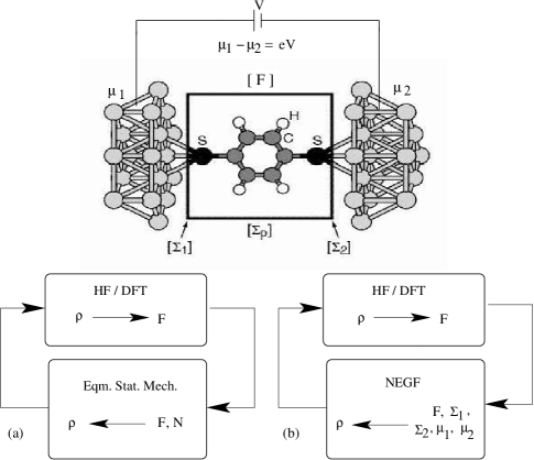
Figure 1: Schematic of a molecule (phenyl dithiol) connected to two semi-infinite gold contacts. The self-energy matrices $\Sigma_{1}$ and $\Sigma_{2}$ exactly account for the contacts and are of the same size as the molecular Fock matrix $F$. The self-consistency scheme is shown for (a) isolated molecule in equilibrium and (b) contact-molecule- contact system under bias.

The electronic structure of an isolated device is obtained in standard quantum chemistry through a self-consistent procedure [32, 33] shown schematically in Fig 1 a. The process consists of two steps that have to be iterated to obtain a self-consistent solution. Step 1: Calculate the Fock matrix $F$ for a given density matrix $\rho$ using a specific scheme such as Hartree-Fock (HF) or density functional theory (DFT) to obtain the self-consistent field , and Step 2: Calculate the density matrix from a given self-consistent Fock matrix $F$ and total number of electrons $N$, based on the laws of equilibrium statistical mechanics.

The problem of calculating the current-voltage (I-V) characteristics is different from the above self-consistent procedure in the following ways : (i) We are dealing with an open system having a continuous density of states and variable (in principle fractional) number of electrons, rather than an isolated molecule with discrete levels and integer number of electrons; (ii) The molecule does not necessarily remain at equilibrium or even close to equilibrium - two volts applied across a short molecule is enough to drive it far from equilibrium; (iii) Surface effects like chemisorption and bonding with the contacts are expected to play a non-trivial role in transport. To calculate the density matrix (step 2 above) we therefore need a method based on non-equilibrium statistical mechanics applicable to such an open system with a continuous density of states. The Non-equilibrium Green’s Function (NEGF) formalism [34, 35] provides us with such a method and that is what we use in this paper for step 2. Step 1, however, remains unchanged and we use exactly the same procedure as in standard quantum chemistry software. The overall procedure is shown schematically in Fig 1 b.

We rigorously partition the contact-molecule-contact system (see Fig 1) into a contact subspace and a device subspace. This makes the molecular chemistry conceptually transparent as well as computationally tractable. The contact subspace is treated via a one-time calculation of the surface Green’s function of the contacts including their atomicity and crystalline symmetry. Different molecules coupled to the same contacts have different couplings but the contact surface Green’s function is independent of the molecule. Given the surface Green’s function and the contact-molecule coupling we can describe the chemisorption and bonding of the molecule with the infinite contacts through self-energy matrices of finite size (equal to that of the molecular subspace). The NEGF formalism has clear prescriptions (Section II) to calculate the non-equilibrium density matrix from a knowledge of $F$, $\Sigma_{1,2}$ and the electrochemical potentials in the two contacts, $\mu_{1}$ and $\mu_{2}$. All quantities of interest (electron density, current etc) are then calculated from the self-consistently converged density matrix.

From a computational viewpoint, the most challenging part is the calculation of the Fock matrix $F$, which involves the core molecular Hamiltonian and the self-consistent potential. A number of researchers have developed their own schemes for performing such ab-initio computations [27, 28, 29]. We accomplish this part by exploiting the fast algorithms of Gaussian ’98 [36], a commercially available quantum chemistry software. Aside from the computational advantages of using an already well-established software, such a close coupling to the standard tools for analyzing molecules makes the chemistry of the system clearer. We describe the contacts and the molecule using the sophisticated LANL2DZ basis set [37, 38] which incorporates relativistic core pseudopotentials. The self-consistent potential is calculated using DFT with Becke-3 exchange [39] and Perdew-Wang 91 correlation [40]. Thus, equipped with a SUN workstation, we are able to perform a parameter-free analysis of conduction in molecular wires in a few hours [41].

We illustrate our method using a gold nanowire and a phenyl dithiol molecule sandwiched between gold contacts and study some previously addressed issues like (1) charge transfer and self-consistent band lineup (e.g. [42]), (2) I-V characteristics (e.g. [18, 20, 27]) and (3) charge density and voltage drop (e.g. [28, 23]). Metallic conduction with quantum unit conductance is observed in the gold nanowire. Upon reducing the coupling to contacts, the gold nanowire exhibits resonant tunneling type of conduction just as seen in a phenyl dithiol molecule. The introduction of a defect (a stretched bond) in the nanowire gives rise to a sharp voltage drop across the impurity as expected. The presence of the defect leads to negative-differential resistance (NDR) in the I-V characteristic of the wire. Periodic Friedel oscillations are observed in the charge density near the defect, the magnitude of these oscillations decreasing as expected upon the introduction of phase-breaking scattering.

This paper is organized as follows. Section II contains a fairly detailed description of the theoretical formulation, specifically modeling the influence of the contacts on the device subspace through self-energy matrices, and developing an appropriate transport formalism to calculate the density matrix $\rho$ (Step 2 above) for the resulting open system under bias. The calculation of the Fock matrix $F$ given the density matrix $\rho$ (Step 1 above) is a standard procedure in quantum chemistry and we will not discuss it further. Section III shows the results and Section IV briefly summarizes the paper.

II Theoretical Formulation

II-A Broadening in an open system: Self-energy.

The concept of self-energy is used in many-body physics to describe non-coherent electron-electron and electron-phonon interactions. We could do the same in principle and use a self-energy function $\Sigma_{p}$ to describe the effect of non-coherent interactions of the molecule with its surroundings (see Fig 1). For the most part of this paper (one exception is made in Fig 11 a, bottom panel), we will neglect such non-coherent scattering processes ($\Sigma_{p}=0$) because the experimental current-voltage characteristics do not show any signatures of the molecular vibration spectra. In addition to $\Sigma_{p}$, we can use self-energy functions $\Sigma_{1}$ and $\Sigma_{2}$ to describe the interactions of the molecule with the two contacts respectively [34].

The contact self-energies $\Sigma_{1}$ and $\Sigma_{2}$ arise formally out of partitioning an infinite system and projecting out the contact Hamiltonians. When an isolated molecule with discrete energy levels is contacted to leads to make an infinite composite system, the energy-dependent one-particle retarded Green’s function of the complete system is expressed in an appropriate basis set as:

$$G(E)=\left[(E+i0^{+})S-F\right]^{-1}$$ (1)

where $S$ is the overlap matrix and $F$ is the Fock matrix for the whole system. $F$ incorporates the effect of external fields, the electronic kinetic energy, electron-nuclear attractions, as well as electron-electron interactions, which could in principle include Coulomb, exchange and correlation effects. The poles of this Green’s function lie near the real energy axis, and represent the energy levels for the infinite system. To extract just the device part of $G$ involving the device overlap matrix $S_{dd}$ and the device Fock matrix $F_{dd}$, we utilize the fact that for a matrix

$$G = (ES-F)^{-1}$$ (5)

$$= \left[\begin{array}[]{ccc}ES_{dd}-F_{dd}&\vdots&\tau\\ \cdots&&\cdots\\ \tau^{\dagger}&\vdots&D\end{array}\right]^{-1}$$

$$= \left[\begin{array}[]{ccc}G_{dd}&\vdots&\\ \cdots&&\cdots\\ &\vdots&\end{array}\right]$$ (9)

the device part $G_{dd}$ is given by $\left(ES_{dd}-F_{dd}-\tau D^{-1}\tau^{\dagger}\right)^{-1}$. $\tau D^{-1}\tau^{\dagger}$ is the self-energy term that describes the effect of the contacts on the device. Only a few surface (interface between device and contact) sites give rise to non-zero coupling elements in $\tau$ [34], and thus only the surface term of $D^{-1}$, the surface Green’s function $g$ is needed. We are thus left with a reduced device Green’s function $G_{dd}$ given by:

$$G_{dd}(E)=\left[ES_{dd}-F_{dd}-\Sigma_{1}(E)-\Sigma_{2}(E)\right]^{-1}$$ (10)

where the self-energy matrices $\Sigma_{1}$ and $\Sigma_{2}$ are non-Hermitian matrices arising from partitioning out contacts 1 and 2 respectively. Each contact self-energy matrix is related to the non-zero part of the corresponding lead-device coupling $\tau$ and the surface Green’s function $g(E)$ through:

$$\Sigma_{1,2}=\tau_{1,2}g_{1,2}\tau_{1,2}^{\dagger}$$ (11)

The geometry of the bonding between the molecule and the contact surface determines the coupling matrices $\tau_{1,2}$. For thiol bonds for example, experimentally it is believed that a chemically bonded sulfur atom on a gold surface overlaps equally with three gold atoms that form an equilateral triangle as shown in Fig 1 [43, 44]. We use the LANL2DZ basis set [37, 38] to describe both the contacts and the molecule. LANL2DZ is a sophisticated basis set with relativistic core pseudopotentials and is observed to provide a good description of the contact surface density of states around the Fermi energy . The coupling matrices $\tau_{1,2}$ are calculated by using Gaussian ’98 to simulate an ‘extended molecule’ [42, 45] consisting of the molecule under consideration and an equilateral triangle of three gold atoms on either side of the molecule.

The surface Green’s function matrices $g_{1,2}$ are obtained recursively for a periodic lattice by the same decimation process as for the device. Removing one layer of the contact lattice gives back the same surface Green’s function, so each contact surface Green’s function satisfies a recursive equation [46] involving on site and coupling matrices $\alpha$ and $\beta$ (diagonal and off-diagonal blocks of $ES-F$ respectively, see Fig 3):

$$g^{-1}=\alpha-\beta g\beta^{\dagger}$$ (12)

To generalize to a 3-D lead of a specific orientation, we follow the procedure in [46] and go to the 2-D $k$-space representation for each cross-sectional plane of the lead, so that each $k$-point effectively acts as an independent 1-D problem for which the above recursive formula holds.

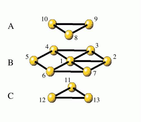
Figure 2: Central $13$ atom part of the 28 atom gold cluster in FCC (111) geometry used to calculate the coupling matrices $S_{mn}$ and $F_{mn}$ in Eq. 13. A reference atom (atom 1) and all it’s nearest neighbors are shown in this central 13 atom part. 28 atoms are used so as to reduce the ‘edge’ effects that tend to destroy the symmetries associated with the Fock matrices $F_{mn}$ (see the discussion following Eq. 13 and Appendix A).

For gold (111) leads, we use Gaussian ’98 to extract in-plane and out-of-plane nearest-neighbor overlap matrix $S$ and Fock matrix $F$ components using a gold cluster (see Fig  2) and define Fourier components in the (111) plane:

$$F_{a\vec{k}}=\sum_{n}F_{mn}e^{-i\vec{k}\cdot(\vec{r}_{m}-\vec{r}_{n})}$$

$$S_{a\vec{k}}=\sum_{n}S_{mn}e^{-i\vec{k}\cdot(\vec{r}_{m}-\vec{r}_{n})}$$ (13)

where $m$ is an arbitrary gold atom, and $n$ involves a sum over $m$ and all its nearest in-plane neighbors, with coordinate $\vec{r}_{n}$. The out-of-plane Fourier components $F_{b\vec{k}}$ and $S_{b\vec{k}}$ are also defined analogously. The $F_{mn}$ and $S_{mn}$ matrices must all obey the group theoretical symmetry of the FCC crystal. This symmetry is satisfied by the $S_{mn}$ matrices since the overlap between two atoms depends only on those two atoms and not on the rest of the atoms in the gold cluster. The $F_{mn}$ matrices, however, are obtained via a self-consistent calculation (see Fig 1 a) and depend on the presence or absence of other atoms in the cluster. Ideally we need to simulate an infinite cluster (or crystal) in order to get the Fock matrices to obey the symmetry. For practical reasons we simulate a finite cluster consisting of 28 gold atoms arranged in the FCC (111) geometry (the central 13 atom part of this cluster is shown in Fig 2) and enforce the known symmetry rules for FCC (111) crystal structure on the resulting Fock matrices. A detailed description of this procedure of enforcing symmetry is given in Appendix A. With the correct symmetry imposed, the $F_{a\vec{k}}$ and $S_{a\vec{k}}$ matrices in Eq. 13 are Hermitian. The gold surface Green’s function in $\vec{k}$ space is then obtained by iteratively solving [46]

$$g^{-1}_{\vec{k}}=\alpha_{\vec{k}}-\beta_{\vec{k}}g_{\vec{k}}\beta^{\dagger}_{\vec{k}}$$ (14)

where

$$\alpha_{\vec{k}}=(E+i0^{+})S_{a\vec{k}}-F_{a\vec{k}}$$

and

$$\beta_{\vec{k}}=(E+i0^{+})S_{b\vec{k}}-F_{b\vec{k}}$$

The real-space gold (111) surface Green’s function matrices are then obtained using

$$g_{mn}=\frac{1}{N}~{}\sum_{\vec{k}}g_{\vec{k}}e^{i\vec{k}\cdot(\vec{r}_{m}-\vec{r}_{n})}$$ (15)

where $N$ is the number of unit cells in the (111) plane (or the number of $k$ points). The surface Green’s function matrices so obtained are independant of the molecule under consideration and depend only on the material and geometry of the contacts.

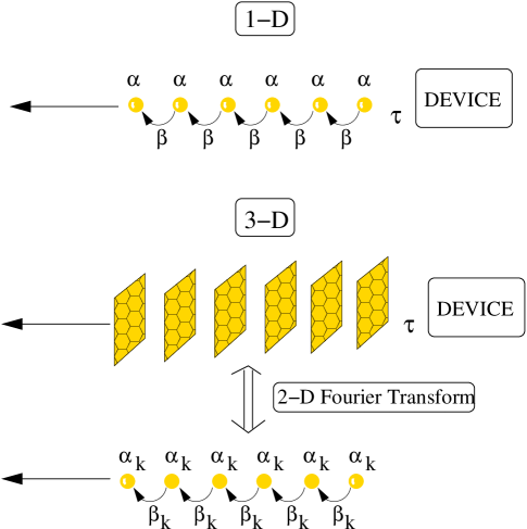
Figure 3: Device coupled to a semi-infinite contact (top: 1-D contact, bottom: 3-D contact). The contact self-energy depends on the device-contact coupling $\tau$ and the contact surface Green’s function $g$ which is recursively solved for by using the contact on-site and coupling matrices $\alpha$ and $\beta$ (see text). In case of a 3-D contact, the in-plane periodicity is used to obtain an equivalent 1-D picture with k-dependent $\alpha_{k}$ and $\beta_{k}$.

We have thus managed to partition the system exactly into a device and a lead subspace. The self-energy matrices replacing the contacts are non-Hermitian, their real parts representing the shift in the molecular energy levels due to coupling with the infinite contacts, and their imaginary parts representing the broadenings of these levels into a continuous density of states. The partitioning makes the problem computationally tractable, since the size of the self-energy matrices is the same as that of the device Fock matrix, even though they represent the effect of infinitely large contacts exactly. In addition, the partitioning decomposes the problem into three different subspaces each involving a different area of research: (i) the device Fock matrix $F_{dd}$ incorporates the quantum chemistry of the intrinsic molecule; (ii) the coupling matrix $\tau$ involves details of the bonding between the molecule and the contact (chemisorption, physisorption etc.) and (iii) the surface Green’s function $g$ involves the surface physics of the metallic contact, which could in principle be extended to include additional effects such as surface states, band-bending, surface adsorption and surface reconstruction.

It is desirable to include a few metal atoms as part of the device for a number of reasons. (i) The molecule may affect a few nearby atoms on the surface of the metallic contact. These surface effects will be automatically accounted for in the self-consistent calculation if a few surface metal atoms are included as part of the device. (ii) Density functional theory is traditionally used for a finite system with an integer number of electrons, or periodic systems. Extending DFT to a non-neutral open molecular subsystem with fractional number of electrons is a topic of intense research [47, 48]. However an extended molecule which includes a few metal atoms is effectively charge neutral and allows the standard DFT formalism to go through. (iii) The charges in the molecule are imaged on the metallic contact. These image charges need to be taken into account in order to accurately calculate the self-consistent potential. It is reasonable to expect that the image charges will reside on a few surface metal atoms that are close to the molecule, and hence the inclusion of these surface atoms in the device should account for the image charge effect on the self-consistent potential. (iv) Finally, the atoms near the two ends of the molecule will have slightly erroneous charge densities because the device and contact basis functions are not orthogonal to each other and the partitioning of charge leads to ambiguities at the interfaces (see Mulliken/Löwdin [49] partitioning). So it is desirable to ‘pad’ the molecule with a few metal atoms on the two ends so as to allow an accurate calculation of the molecular charge.

The results we present in this paper are obtained using just the molecule as our ‘device’ (metal atoms are not included in the device) in order to reduce the computational time. Preliminary calculations indicate that including the metal atoms improves certain aspects such as the charge density on the end atoms. However, such a calculation with an extended device takes much more computer time, especially with gold contacts.

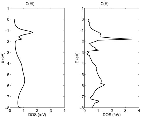
Figure 4: Comparison of non-self-consistent evaluations of DOS for phenyl dithiol with and without a constant self-energy approximation. The excellent correspondence is a consequence of the relatively flat DOS of Au(111) near the Fermi energy.

The energy dependent self-energy matrices discussed above exactly account for the bonding and chemisorption of the molecule onto the contact surface, as we discuss in our results section. For gold (111) contacts we find that these issues are taken care of even if we replace $\Sigma(E)$ with $\Sigma(E_{f})$ ($E_{f}$ is the gold Fermi energy) as is evident from Fig. 4. This helps to reduce the time taken to compute the density matrix (see Eq. 16). We have developed a fast and elegant analytical method to evaluate the density matrix for an energy independent self-energy. This method is explained in Appendix B. Such a simplification may not be possible for platinum contacts having a significant structure in the density of states near $E_{f}$. This makes the calculation of the density matrix computationally quite challenging because the correlation function may have sharp peaks in the range of integration. Integrating over a complex energy contour [42, 50] simplifies the computational complexity to a certain degree, but the energy range of integration has to be huge in order to take into account all the molecular levels (see Appendix B), and a faster scheme is desirable.

II-B Transport: Non-equilibrium Green’s function (NEGF) formalism.

The NEGF formalism provides a suitable method for calculating the density matrix $\rho$ for systems under non-equilibrium conditions. A tutorial description of this formalism can be found in [35]. Here we will simply summarize the basic relations that can be used (1) to obtain $\rho$, given the molecular Fock matrix $F$, the self-energy matrices $\Sigma_{1}$, $\Sigma_{2}$, and the contact electrochemical potentials $\mu_{1}$ and $\mu_{2}$ and (2) to obtain the electron density $n(\vec{r}$) and current $I$ from the self-consistent density matrix $\rho$. For open systems with a continuous density of states, the density matrix can be expressed as an energy integral over the correlation function $-iG^{<}(E)$, which can be viewed as an energy-resolved density matrix:

$$\rho=\int dE[-iG^{<}(E)/2\pi]$$ (16)

The correlation function is obtained from

$$-i{G}^{<}=G\left({f_{1}\Gamma_{1}+f_{2}\Gamma_{2}}\right)G^{\dagger}$$ (17)

where $f_{1,2}(E)$ are the Fermi functions with electrochemical potentials $\mu_{1,2}$

$$f_{1,2}(E)=\left(1+\exp{\left[{{E-\mu_{1,2}}\over{k_{B}T}}\right]}\right)^{-1}$$ (18)

G is the Green’s function matrix (energy-dependent) in a non-orthogonal basis:

$${G}=\left(ES-F-{\Sigma}_{1}-{\Sigma}_{2}\right)^{-1}$$ (19)

where $S$ is the overlap matrix. The broadening functions are the anti-Hermitian components of the self-energy:

$${\Gamma}_{1,2}=i[{\Sigma}_{1,2}-{\Sigma}_{1,2}^{\dagger}]$$ (20)

The NEGF equation for $\rho$ can be interpreted as the filling of broadened energy levels (eigenvalues of $F$) by two separate contacts, with $G\Gamma_{i}G^{\dagger}$ representing the density of states (DOS) contribution from the $i$th electrode, and $f_{i}$ representing the Fermi function of the $i$th electrode. Eq. 17 assumes that the contacts are reflectionless [34].

The converged (see Fig 1 b) density matrix is used to obtain the total number as well as the spatial distribution of electrons using

$$N = {\rm trace}(\rho S)$$

$$n(\vec{r}) = \sum_{m,n}\rho_{mn}\phi_{m}(\vec{r})\phi_{n}(\vec{r})$$ (21)

where $\phi_{m,n}(\vec{r})$ represent molecular basis functions. The converged density matrix may also be used to obtain the terminal current [34]. For coherent transport , we can simplify the calculation of the current by using the transmission formalism where the transmission function [34]:

$$T(E)={\rm trace}\left[\Gamma_{1}G\Gamma_{2}G^{\dagger}\right]$$

is used to calculate the terminal current

$$I=(2e/h)\int_{-\infty}^{\infty}dE~{}T(E)~{}\left(f_{1}(E)-f_{2}(E)\right)$$ (22)

III Results

III-A Equilibrium

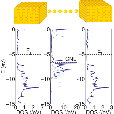
Figure 5: Charge transfer and self-consistent band lineup upon coupling a gold nanowire to two gold contacts. The charge neutrality level (CNL) of the wire lies below the Fermi energy of gold, leading to electron flow from contacts to the wire. The DOS (dashed) of the charge-neutral wire redistributes and floats up (solid) self-consistently due to charging energies associated with the electron flow.

Charge transfer and band lineup. The charge transferred between a device and contacts leads to aligning of reference energy levels in the two subsystems. Such band lineup issues are of primary importance in understanding semiconductor heterojunctions as well as plastic electronics. An analogous band-lineup diagram can be obtained on coupling a molecule to contacts. Fig 5 shows the surface DOS of the contacts and the DOS of the device (a gold nanowire in this case). The 6 atom gold chain has discrete energy levels that are broadened into a metallic band-like DOS on coupling to contacts. For the chain with a broadened density of states, one can define a charge-neutrality level (CNL) [53], such that filling up all the states below the CNL keeps the device charge-neutral. The Fermi energy of gold, approximately -5.1 eV (negative of the bulk gold work function), is noticeably higher than the CNL of a 1-D gold nanowire. Owing to this difference electrons flow in from the contacts to the device. For a small molecule, the capacitative charging energy is large, so the original broadened levels (dashed) float up self-consistently (solid) due to charging till the charge transfer ceases, the band lineup is complete and the device and contacts are in chemical equilibrium.

III-B Non-equilibrium

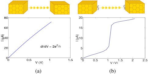
Figure 6: (a)I-V of a Gold nanowire with six gold atoms forming a 1-D chain connected to two gold contacts. An energy-independent self-energy $\Sigma(E_{f})$ is used to model the contacts. A quantum unit conductance of $2e^{2}/h$ signifies that $\Sigma(E_{f})$ accounts for the perfect transmission by seamlessly joining the nanowire to the contacts. (b) I-V of the same gold nanowire but with reduced contact coupling which decreases level broadening and a resonant tunneling type conduction is seen. The I-V shows step-like behavior with the current jumping up when the contact Fermi levels $\mu_{1}$ and/or $\mu_{2}$ cross a molecular level (See Figs 7, 8).

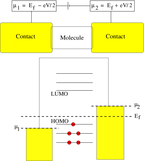
Figure 7: Mechanism explaining how current flows through a molecule coupled to contacts. At equilibrium ($V=0$) $\mu_{1}=\mu_{2}=E_{f}$ and no current flows. For non-zero $V$ the contact Fermi energies separate by an amount $eV$ and a significant current flows only when a molecular level lies in between $\mu_{1}$ and $\mu_{2}$ (also see Fig 8).

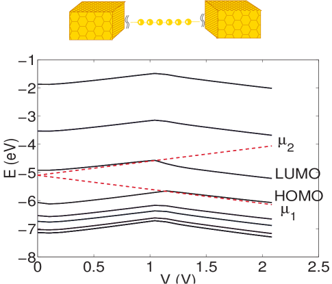
Figure 8: Energy levels of a gold nanowire weakly coupled to contacts as a function of applied bias. The I-V for this case is shown in Fig 6 b. At zero bias the contact Fermi level is close to LUMO. At non-zero bias $\mu_{2}$ wants to fill up the LUMO and add extra electrons in the device, so charging effects tend to float the levels up till $\mu_{1}$ comes close to HOMO and wants to empty it. At this point, more electrons are lost than gained and charging effects make the levels float down parallel to $\mu_{1}$ in order to minimize the loss of electrons.

I-V characteristics. A gold nanowire connected to gold contacts has a continuous DOS near the equilibrium Fermi energy (see Fig 5, middle panel), and hence we expect it to exhibit metallic conduction as shown in Fig 6 a. The nanowire exhibits a conductance equal to the quantum unit conductance of $2e^{2}/h\approx 77\mu S$. This ohmic I-V is a testimony to the accuracy of our self-energy matrix. Only a correct self-energy matrix will get rid of spurious reflections at the contact and seamlessly couple the 1-D gold wire with the 3-D gold contact. Fig 6 b shows the I-V characteristic for the same gold nanowire, but with the coupling to the contacts reduced by a factor of 4. Due to the reduced coupling, the broadening of the levels is much less than the separation between the levels, and the wire now exhibits resonant conduction [41]. There are marked plateaus in the I-V curve when a level lies between the contact Fermi levels. This is shown schematically in Fig 7. Fig 8 shows the energy levels of the weakly coupled gold nanowire as a function of applied bias. At equilibrium, the contact Fermi level lies close to the LUMO level. For a non-zero bias $V$, $\mu_{1}$ and $\mu_{2}$ separate by an amount $eV$ .$\mu_{2}$ moves closer to LUMO and wants to fill it up. Charging effects now come into the picture and the levels tend to float up and follow $\mu_{2}$ until $\mu_{1}$ comes close to crossing the HOMO level. At this point, $\mu_{2}$ wants to put charge into the LUMO while $\mu_{1}$ wants to empty the HOMO. The number of electrons lost is more than the number gained, and now the levels tend to go down with $\mu_{1}$ in order to prevent further loss of electrons. The current jumps up (see Fig 6 b) at that bias point where $\mu_{2}$ crosses the LUMO level. Such resonant conduction is also seen in a phenyl dithiol molecule (Fig 10) with pronounced peaks in the conductance $dI/dV$ at resonance.

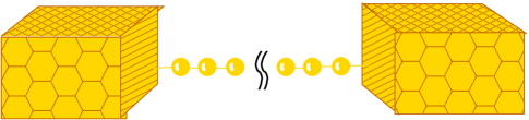
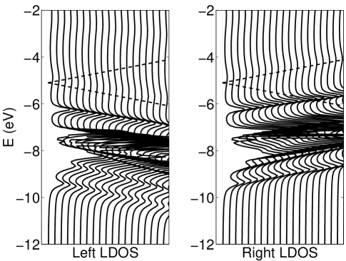
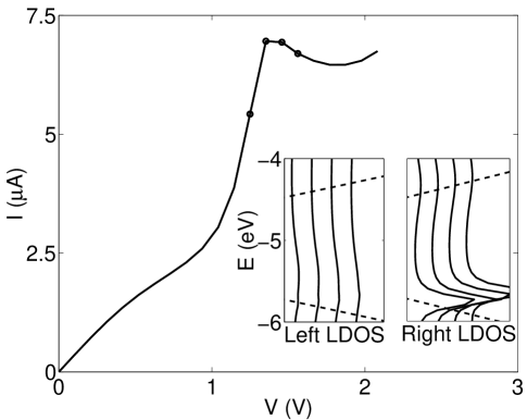
Figure 9: Left and right LDOS for a wire with a defect in the center for 21 equidistant voltage values from 0 to 2 volts, laterally shifted equally for clarity. The electrons in the left and right segments of the wire are separately in equilibrium with the left and right contacts, and their respective LDOS follow the corresponding contact electrochemical potentials (dashed lines) because of charging effects similar to those seen in Fig 8. As the two LDOS slide past each other within the $\mu_{1}$-$\mu_{2}$ window (shown magnified in the inset of the bottom figure at the four voltage points circled in the I-V graph) their peak values (tail of the peak for the left LDOS) come in and out of resonance, producing thereby a weak NDR in the I-V characteristic.

The I-V characteristic for a quantum point contact with a defect at the center exhibits a weak negative differential resistance (NDR) (Fig 9). We artificially stretch a bond in the middle of our 6 atom gold chain, which causes the left and right local density of states (LDOS) of the chain to separately be in equilibrium with the left and right contacts. Applying a bias then causes the two LDOS to sweep past each other within $\mu_{1,2}$. Owing to the presence of some sharp van-Hove singularities in the DOS and some smoothened out maxima, there is a progressive alignment and misalignment of peaks in the LDOS that leads to a weak NDR in the I-V. A similar mechanism for NDR has been observed in other calculations [29, 19].

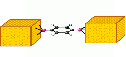
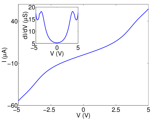
Figure 10: I-V of phenyl dithiol connected to two gold contacts. The underlying mechanism is resonant tunneling - much like that in a gold nanowire weakly coupled to the contacts (see Fig 6 b). The gap depends on the proximity of the Fermi energy to the zero bias HOMO level if we neglect charging effects, while the maximum current at the onset of conduction is proportional to the parallel combination of broadenings at the molecular energy (see text). For phenyl dithiol, the predictions from the above estimates are about 4 volts and 40 $\mu$A respectively.

Although most semi-empirical theories qualitatively match the shape of the resonant I-V characteristics for molecular conductors such as phenyl dithiol (PDT), quantitative agreements between experiment and theory have been largely unsatisfactory. The I-V for PDT can be quantified by the conductance gap and the current value at the onset of conduction. If we neglect the charging energy $U_{c}$ the gap is roughly given by the proximity of the contact Fermi energy to the nearest conducting molecular level, $E_{gap}\approx 4|E_{f}-E_{mol}|$ [8]; while the peak current at the onset of conduction is roughly given by $2e\Gamma_{1}\Gamma_{2}/\left(\Gamma_{1}+\Gamma_{2}\right)\hbar$, evaluated at the energy $E_{mol}$. The current onset is smeared out over the tail of the molecular level, which in conjunction with charging effects leads to a rise in current at the molecular level crossing extended over a voltage width $\Delta V\approx\left(\Gamma_{1}+\Gamma_{2}+U_{C}\right)/e$. Ab-initio theories are indispensable for obtaining self-consistently the position of the Fermi energy relative to the molecular levels, as well as the broadenings of the levels. Both from ab-initio calculations for PDT, as well as ab-initio estimates based on the above arguments, the predicted conductance gap of PDT, set by the molecular HOMO level, comes out to about 4 Volts, while the maximum current turns out to be tens of microamperes. Experimentally both the conductance gap and the maximum current are much less than these theoretical estimates. The decrease in current can be attributed either to weak coupling between molecular $\pi$ orbitals and the s-orbitals of loose gold atoms at the contact surface [54, 27], or to tunneling between molecular units separately chemisorbed on two ends of a break-junction [55]. Thus a precise experimental knowledge of the contact conditions is essential prior to appropriate surface modeling. The conductance gap is as yet unexplained by the above attempts, and requires once again a precise knowledge of contact surface conditions which can vary the Fermi energy substantially enough to alter the conductance gap.

Voltage drop and electron density. An applied voltage is known to drop largely across the metal-molecule interface, leading to a weaker drop in the molecule. The precise nature of the potential profile is an important input to semi-empirical calculations of transport. Tian et al. [18] suggested using a flat potential profile inside the molecule, with a voltage division factor describing its position. Such a flat profile was obtained by Mujica et al. [23] by solving a 1-D Poisson equation, and experimentally measured for longer ($\sim\mu$m) wires by Seshadri and Frisbie [56]. However, in all these cases the geometry under consideration is a series of 2-D charge sheets with potential variations only along the wire axis. The 1-D Poisson equation allows variations only along one coordinate, while the measurements in [56] referred to a self-assembled monolayer (SAM) where once again transverse potential variations are screened out by the presence of neighboring molecules. In contrast, Lang and Avouris [28] obtained a significant potential drop in a carbon atomic wire, which is a consequence of fields penetrating from transverse directions, as correctly predicted for a break-junction geometry by a 3-D Poisson equation. Our particular geometry is suited to the break-junction, since the Hartree term in Gaussian ’98 is calculated for a 3-D geometry.

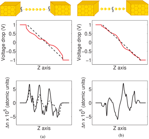
Figure 11: Electrostatics of (a) a weakly contacted gold wire, and (b) a strongly contacted wire with a substitutional defect (a stretched bond at the center), in response to a 2 volt applied bias across the contacts. Top panel: schematic, middle panel: voltage drop along the wire (dashed lines show a linear drop for comparison), bottom panel: density of electrons along the wire. In all plots, the corresponding quantities at equilibrium have been subtracted out in order to remove peaks near the positions of the nuclei for clarity. There is a substantial voltage drop in the wires due to transverse fields penetrating the thin (single atom cross-section) conductors. The largest potential drop is at the barriers (wire-metal interfaces and defects), while the electronic charge piles up against the applied bias as expected. Superposed on this general polarization of charge are Friedel oscillations, which die out (dashed line in left bottom panel) on increasing incoherent scattering in the wire, incorporated through an additional phonon self-energy $\Sigma_{p}$ introduced through a Büttiker probe.

Fig 11 a shows a gold nanowire weakly coupled to the contacts. In Fig 11 b, the coupling to contacts is strong, but a substitutional defect has been incorporated by artificially introducing a bond that is longer than the equilibrium gold bond length. The voltage drop across the device itself is smaller than the applied voltage bias owing to screening effects, incorporated self-consistently through the Hartree term of our Fock matrix. The plots on top show the net self-consistent voltage drop across the wire (solid lines). The electrostatic potential does not exhibit peaks at the atomic positions because the equilibrium potential profile has been subtracted for clarity. Shown for comparison is the linear voltage drop (dashed lines), the solution to Laplace’s equation in the region. In (b), a large part of the voltage drop occurs at the defect as expected. In (a) one might ask why the voltage drops across a ballistic device. It is important to recognize the distinction between the electrostatic potential and the electrochemical potential at this point. In a ballistic device, it is the electrochemical potential that remains constant due to absence of scattering. The electrostatic potential, however, obeys Poisson’s equation and may or may not vary depending on the charge density inside the device. For example, a vacuum tube is a ballistic device with a linear voltage (electrostatic potential) drop due to the absence of any charge. The potential is not well screened out due to the thin (one atom) cross-section of the wire, which allows transverse fields to penetrate. In contrast, in a self-assembled monolayer (SAM), the potential variation is expected to resemble that predicted in [18]. However, this requires us to disable the Hartree term in Gaussian ’98 and replace it with our own evaluation (this is under current investigation).

The transferred number of electrons (Fig 11, bottom panels) $\Delta n$ along the wire obtained from our self-consistent solution shows how the voltage drops develop. In both plots, there are sizeable oscillations in the charge density, which we identify as Friedel oscillations. The equilibrium electron density is $n=1/d$ for the wire ($d$ is the spacing between atoms in the wire), leading to a 1-D Fermi wave-vector $k_{F}=n\pi/2=\pi/2d$. The corresponding Friedel oscillation wavelength is $2\pi/(2k_{F})=2d$, about twice an interatomic spacing, predicting about three oscillation cycles in a six atom device, as we indeed observed. Furthermore, the amplitudes of the oscillations decrease on incorporating an incoherent scattering process in the wire through a Büttiker probe [51] (which shows up as an additional self-energy matrix $\Sigma_{p}$ representing coupling of the wire with a phonon-bath, for example). Superposed on the Friedel oscillations is the general trend of the charge distribution, to flow against the applied field (i.e., piling to the left). In (a) this piled up electronic charge screens the applied field and reduces the slope of the voltage drop in the wire. In (b), the charge piles up on each side of the barrier, leading to a charge resistivity dipole in the center. This dipole has a polar field that is now in the direction of the applied field, thus increasing the voltage drop across the barrier .

IV Summary

In this paper we have described a straightforward but rigorous procedure for calculating the I-V characteristics of molecular wires. The Fock matrix is obtained using a Gaussian basis set (LANL2DZ) and the self-consistent potential is obtained using density functional theory with the B3PW91 approximation. This approach is identical to that used in standard quantum chemistry programs like Gaussian ’98. The difference lies in our use of the NEGF formalism to calculate the density matrix from the Fock matrix. This allows us to handle open systems far from equilibrium which are very different from the isolated molecules commonly modeled in quantum chemistry. The close coupling with standard quantum chemistry programs not only makes the procedure simpler to implement but also makes the relation between the I-V characteristics and the chemistry of the molecule more obvious. Partitioning the contact-molecule-contact system into a molecular subspace and a contact subspace allows us to focus on the quantum chemistry of the molecule while exactly taking into account the bonding of the molecule with the contacts, contact surface physics and atomicity etc. We use our method to interpolate between two extreme examples of transport through a molecular wire connected to gold contacts: band conduction in a metallic (gold) nanowire, and resonant conduction through broadened, quasidiscrete levels of a phenyl dithiol molecule. We examine quantities of interest like the I-V characteristic, voltage drop and charge density.

We would like to thank F. Zahid, U. Savagaonkar, M. Paulsson, T. Rakshit and R. Venugopal for useful discussions. This work was supported by NSF and the US Army Research Office (ARO) under grants number 9809520-ECS and DAAD19-99-1-0198.

Appendix A       Self-energy: Imposing the FCC (111) Symmetry

In order to calculate the gold (111) surface Green’s function, we use Gaussian ’98 to simulate a 28 atom gold cluster with FCC (111) geometry and then extract the in-plane and out-of-plane overlap and Fock matrix components $S_{mn}$ and $F_{mn}$ (see the discussion following Eq. 13 in Section II). The cluster, however, does not have the full group theoretical symmetry of the FCC (111) crystal due to edge-effects. This symmetry needs to be imposed on the extracted Fock matrix elements in order to be consistent with the assumptions of two-dimensional periodicity that go into our $\vec{k}$-space formalism. The overlap matrix elements automatically satisfy these symmetry requirements, since they involve products of two on-site localized orbitals.

A typical cluster is shown in Fig 2, with atoms numbered from 1 to 13. An FCC (111) surface consists of repetitions of such clusters in the sequence ABCABCABC $\ldots$, B being the plane numbered 1 to 7, and A and C being the planes with the rotated triangles above and below it. Each plane is parallel to the x-y plane, atom 1 is at the origin and atom 2 lies on the x-axis. This gives us a $z$-axis in the (111) direction, along which the molecule is assumed to align after contacting with the Au surface. The Fock matrix for the cluster looks as follows:

$$F=\left[\begin{array}[]{cccc}F_{11}&F_{12}&\cdots&F_{1,13}\\ F_{21}&F_{22}&\ldots\\ \ldots\\ \ldots\\ \ldots\end{array}\right]$$ (23)

The LANL2DZ basis for gold consists of three sets of s, three sets of p and 2 sets of d orbitals, giving us $3+3\times 3+2\times 5=22$ orbitals on each gold atom. Each of the above matrix components $F_{11}$, $F_{12}$ etc. is therefore 22 $\times$ 22 in size. Using Gaussian ’98, we can extract all these matrix components separately. For a Au(111) surface, however, the elements should be interrelated by the point group symmetries of the FCC crystal. Starting with two independent matrix components, say, an on-site element $F_{11}$ that is characteristic of the gold atom, and a nearest neighbor element $F_{12}$ that depends on the lattice parameter, we construct the rest of the elements of $F$ using the symmetry operations.

The FCC crystal has the following symmetry: on rotating the cluster in Fig. 2 by 60 degrees about the $z$-axis followed by a reflection in the x-y plane, we get back the same cluster. This means there is a unitary matrix $M$ that takes $F_{12}$ into $F_{13}$ and so on. The matrix $M$ can be block-decomposed into contributions from each of the s, p and d orbital subspaces. Since s orbitals are spherically symmetric, the corresponding block for the 3 s orbitals is the 3 $\times$ 3 identity matrix. For p orbitals, the $M_{p}$ matrix consists of the following reflection (R) and rotation (U) matrices:

$$M_{p} = R_{p}U_{p}$$

$$R_{p} = \left(\begin{array}[]{ccccc}1&&0&&0\\ 0&&1&&0\\ 0&&0&&-1\end{array}\right)$$ (27)

$$U_{p} = \left(\begin{array}[]{ccccc}\cos{\pi/3}&&-\sin{\pi/3}&&0\\ \sin{\pi/3}&&\cos{\pi/3}&&0\\ 0&&0&&1\end{array}\right)$$ (31)

A similar matrix can be constructed for the d-orbital subspace. At the end of the process we thus get a 22 $\times$ 22 $M$ matrix describing rotation-reflection of the entire LANL2DZ basis set.

The nearest neighbor in-plane couplings of atom 1 can now be generated by repeated applications of the rotation-reflection transformation:

$$F_{17} = M^{\dagger}F_{12}M$$

$$F_{16} = M^{\dagger}F_{17}M$$

$$F_{15} = M^{\dagger}F_{16}M$$

$$F_{14} = M^{\dagger}F_{15}M$$

$$F_{13} = M^{\dagger}F_{14}M$$

$$F_{12} = M^{\dagger}F_{13}M$$ (32)

A simple out-of-plane rotation by 120 degrees can generate $F_{18}$ from $F_{12}$ . Once again, we explicitly write down the contribution for the p orbitals. The d orbitals need to be considered analogously while the s orbitals remain unchanged.

$$F_{18} = (M^{\prime})^{\dagger}F_{12}M^{\prime}$$

$$M^{\prime}_{p} = \left(\begin{array}[]{ccccc}-1/2&&-1/2\sqrt{3}&&\sqrt{2/3}\\ 1/2\sqrt{3}&&5/6&&\sqrt{2}/3\\ -\sqrt{2/3}&&\sqrt{2}/3&&-1/3\end{array}\right)$$ (36)

All the other matrix components can be similarly obtained, using translation and rotation-reflection invariance. For example:

$$F_{1,12} = M^{\dagger}F_{18}M$$

$$F_{1,10} = M^{\dagger}F_{1,12}M$$

$$F_{22} = F_{11}$$

$$F_{23} = F_{14}$$ (37)

and so on.

The crystalline symmetries also constrain the structures of the two fundamental matrix components $F_{11}$ and $F_{12}$ out of which all other components are constructed. $F_{11}$ is a diagonal block of $F$ and is Hermitian. $F_{12}$ satisfies the following condition:

$$\left(M^{\dagger}\right)^{3}F_{12}M^{3}=F_{12}^{\dagger}$$ (38)

Three operations of the rotation-reflection transformation (equivalently, a coordinate inversion) on $F_{12}$ generates the matrix $F_{15}$, which equals $F_{51}^{\dagger}$ by bond-inversion symmetry. Translational symmetry implies $F_{51}=F_{12}$, which leads to the above equation. The form of $F_{12}$ consistent with the above condition is given by:

$$F_{12}=\left(\begin{array}[]{ccc}a&b&c\\ -b^{\dagger}&e&d\\ c^{\dagger}&-d^{\dagger}&f\end{array}\right)$$ (39)

where $a$, $e$ and $f$ are hermitian matrices. The $F_{12}$ matrix extracted from Gaussian will have this structure for a large enough cluster, else we need to impose this condition as well.

With a properly symmetrized set $F_{mn}$ and $S_{mn}$, the matrices $F_{a\vec{k}}$ and $S_{a\vec{k}}$ in Eq. 13 are Hermitian as expected, and we may proceed to calculate the gold (111) surface Green’s function as outlined in Section II. Ignoring the symmetries, however, can lead to non-physical results, including negative density of states or unsymmetric Green’s function matrices.

Appendix B       Density Matrix: Analytical Integration

We have developed a fast and elegant algorithm to evaluate the density matrix given an energy independent self-energy. For bulk gold it is known that around the Fermi energy the local DOS is approximately a constant [57]. It is reasonable to expect that all the transport properties of the molecule are determined by the molecular levels near $E_{f}$ and the deep levels contribute to the total number of electrons by remaining full in the bias range of interest. In view of this, We split the energy range of integration in two parts and denote the boundary by $E_{b}$. $E_{b}$ is chosen such that it is a few electron-volts below the Fermi energy $E_{f}$ and the molecular density of states at $E_{b}$ is negligible. We replace $\Sigma(E)$ by $\Sigma(E_{f})$ in the energy range between $E_{b}$ to $E_{f}$. For the energy range from $-\infty$ to $E_{b}$ we replace $\Sigma(E)$ by $-i\eta$, a constant infinitesimal broadening. The only energy dependence in the integrand in Eq. 16 now appears through the Green’s function $G$ and we can perform an analytical integration in an appropriate eigenspace, as explained below.

To evaluate the density matrix, we now need to solve integrals of the type (see equations 16 through 20 in Section II)

$$2\pi\rho=\int_{-\infty}^{\infty}dE~{}f(E)~{}G(E)~{}\Gamma~{}G^{\dagger}(E)$$ (40)

where $\Gamma$ is the anti-hermitian part (see Eq. 20) of the energy independent self-energy and $f(E)$ is the Fermi function with some electrochemical potential $\mu$ (see Eq. 18). In this paper we assume $T=0~{}K$ which modifies the integral in the above equation as

$$2\pi\rho=\int_{E_{min}}^{\mu}dE~{}G(E)~{}\Gamma~{}G^{\dagger}(E)$$ (41)

where it is understood that $E_{min}$ tends to $-\infty$. Using Eq. 19 for $G(E)$ we may rewrite the above equation as

$$2\pi\rho=S^{-\frac{1}{2}}\left[\int_{E_{min}}^{\mu}dE~{}\overline{G}(E)~{}\overline{\Gamma}~{}\overline{G}^{\dagger}(E)\right]S^{-\frac{1}{2}}$$ (42)

where $S$ is the overlap matrix $\overline{\Gamma}$ and $\overline{G}(E)$ are defined as

$$\overline{\Gamma}=S^{-\frac{1}{2}}\Gamma S^{-\frac{1}{2}}$$

and

$$\overline{G}(E)=\left(EI-\overline{F}\right)^{-1}$$

with $I$ being the identity matrix and

$$\overline{F}=S^{-\frac{1}{2}}\left(F+\Sigma_{1}+\Sigma_{2}\right)S^{-\frac{1}{2}}$$

In the above equation, $\Sigma_{1,2}$ are the energy independent self-energy matrices as discussed at the beginning of this appendix and $F$ is the molecular Fock matrix.

To solve the integral in Eq. 42 analytically, we work in the eigenspace of the energy independent non-Hermitian matrix $\overline{F}$ given by the above equation. Since $\overline{F}$ is non-Hermitian, we need its eigenkets $\{|m\rangle\}$ and their dual kets $\{|\tilde{m}\rangle\}$ in order to form a complete basis set. The corresponding eigenvalues are then $\{\epsilon_{m}\}$ and $\{\epsilon^{*}_{m}\}$. Expanding in this mixed basis set, we get

$$2\pi\rho$$

$$= S^{-\frac{1}{2}}\int_{E_{min}}^{\mu}dE~{}\overline{G}(E)\left(\sum_{p}|p\rangle\langle\tilde{p}|\right)$$

$$\times \overline{\Gamma}~{}\overline{G}^{\dagger}(E)\left(\sum_{q}|\tilde{q}\rangle\langle q|\right)S^{-\frac{1}{2}}$$

$$= S^{-\frac{1}{2}}\left[\sum_{pq}\overline{\Gamma}_{\tilde{p}\tilde{q}}|p\rangle\langle q|\int_{E_{min}}^{\mu}{{dE}\over{\left(E-\epsilon_{p}\right)\left(E-\epsilon^{*}_{q}\right)}}\right]S^{-\frac{1}{2}}$$

where we used $\overline{G}(E)|m\rangle=|m\rangle/(E-\epsilon_{m})$ and $\overline{G}^{\dagger}(E)|\tilde{m}\rangle=|\tilde{m}\rangle/(E-\epsilon^{*}_{m})$.

It is now straightforward to do the above integral analytically and obtain the density matrix. The current $I$ given by Eq. 22 may also be evaluated analytically using a similar procedure. This analytical procedure allows us to do the integration extremely fast and avoids errors arising out of a numerical integration over a grid.

References

- [1] For a review of the experimental work see M.A. Reed, Proc. IEEE 87 (1999) 652.
- [2] A. Yazdani, D. Eigler, N. Lang, Science 272 (1996) 1921.
- [3] C. Collier, E. Wong, M. Belohradsky, F. Raymo, J. Stoddart, P. Kuekes, R. Williams, J. Heath, Science 285 (1999) 391.
- [4] J. Chen, M. Reed, A. Rawlett, J. Tour, Science 286 (1999) 1550.
- [5] M. Reed, C. Zhou, C. Muller, T. Burgin, J. Tour, Science 278 (1997) 252.
- [6] C. Zhou, M. Deshpande, M. Reed, L. Jones, J. Tour, Appl.Phys.Lett. 71 (1997) 2857.
- [7] R. Andres, T. Bein, M. Dorogi, S. Feng, J. Henderson, C. Kubiak, W. Mahoney, R. Osifchin, R. G. Reifenberger, Science 272 (1996) 1323.
- [8] S. Datta, W. Tian, S. Hong, R. Reifenberger, J. I. Henderson, C. Kubiak, Phys. Rev. Lett. 79 (1997) 2530.
- [9] U. Durig, O. Zuger, B. Michel, L. Haussling, H. Ringsdorf, Phys. Rev. B 48 (1993) 1711.
- [10] C. Boulas, J. Davidovits, F. Rondelez, D. Vuillaume, Phys. Rev. Lett. 76 (1996) 4797.
- [11] H. Ohnishi, Y. Kondo, K. Takayanagi, Nature 395 (1998) 780.
- [12] A. Yanson, G. Bollinger, H. van den Brom, N. Agrait, J. van Ruitenbeek, Nature 395 (1998) 783.
- [13] C. Dekker, Phys. Today 52 (1999) 22.
- [14] H. Fink, C. Schonenberger, Nature 398 (1999) 407.
- [15] D. Porath, A. Bezryadin, S. de Vries, C. Dekker, Nature 403 (2000) 635.
- [16] M. Ratner, Nature 397 (1999) 480.
- [17] J. Schön, H. Meng, Z. Bao, Nature 413 (2001) 713.
- [18] W. Tian, S. Datta, S. Hong, R. Reifenberger, J. I. Henderson, C. Kubiak, J. Chem. Phys. 109 (1997) 2874.
- [19] M. Paulsson, S. Stafström, Phys. Rev. B 64 (2001) 035416.
- [20] E. Emberly, G. Kirczenow, Phys. Rev. B 58 (1998) 10911.
- [21] L. E. Hall, J. R. Reimers, N. S. Hush, K. Silverbrook, J. Chem. Phys. 112 (2000) 1510.
- [22] S. Yaliraki, A. Roitberg, C. Gonzalez, V. Mujica, M. Ratner, J. Chem. Phys. 111 (1999) 6997.
- [23] V. Mujica, A. Roitberg, M. Ratner, J. Chem. Phys. 112 (2000) 6834.
- [24] C. Tsu, R. Marcus, J. Chem. Phys. 106 (1997) 584.
- [25] M. Magoga, C. Joachim, Phys.Rev. B 56 (1997) 4722.
- [26] A. Onipko, Phys. Rev. B 59 (1999) 9995.
- [27] M. Di Ventra, S.T. Pantelides and N.D. Lang , Phys. Rev. Lett. 84 (2000) 979.
- [28] N. Lang, P. Avouris, Phys. Rev. Lett. 84 (2000) 358.
- [29] B. Larade, J. Taylor, H. Mehrez, H. Guo, Phys. Rev. B 64 (2001) 075420.
- [30] J. Seminario, A. Zacarias, J. Tour, J.Phys.Chem. A 103 (1999) 7883.
- [31] J. J. Palacios, A. J. Pérez-Jiménez, E. Louis and J. A. Vergés, cond-mat/0101359.
- [32] A. Szabo, N. Ostlund, Modern Quantum Chemistry, Dover Publications, Inc., Mineola, New York, 1996.
- [33] F. Jensen, Introduction to Computational Chemistry, Wiley, 1999.
- [34] S. Datta, Electronic Transport in Mesoscopic Systems, Cambridge University Press, 1995.
- [35] S. Datta, Superlattices and Microstructures 28 (2000) 253.
- [36] Gaussian 98 (Revision A.7), M. J. Frisch, G. W. Trucks, H. B. Schlegel, G. E. Scuseria, M. A. Robb, J. R. Cheeseman, V. G. Zakrzewski, J. A. Montgomery, Jr., R. E. Stratmann, J. C. Burant, S. Dapprich, J. M. Millam, A. D. Daniels, K. N. Kudin, M. C. Strain, O. Farkas, J. Tomasi, V. Barone, M. Cossi, R. Cammi, B. Mennucci, C. Pomelli, C. Adamo, S. Clifford, J. Ochterski, G. A. Petersson, P. Y. Ayala, Q. Cui, K. Morokuma, D. K. Malick, A. D. Rabuck, K. Raghavachari, J. B. Foresman, J. Cioslowski, J. V. Ortiz, A. G. Baboul, B. B. Stefanov, G. Liu, A. Liashenko, P. Piskorz, I. Komaromi, R. Gomperts, R. L. Martin, D. J. Fox, T. Keith, M. A. Al-Laham, C. Y. Peng, A. Nanayakkara, C. Gonzalez, M. Challacombe, P. M. W. Gill, B. G. Johnson, W. Chen, M. W. Wong, J. L. Andres, M. Head-Gordon, E. S. Replogle and J. A. Pople, Gaussian, Inc., Pittsburgh PA (1998).
- [37] P. Hay, W. Wadt, J. Chem. Phys. 82 (1985) 270.
- [38] P. Hay, W. Wadt, J. Chem. Phys. 82 (1985) 284.
- [39] A. D. Becke, J. Chem. Phys. 98 (1993) 5648.
- [40] J. P. Perdew, in: P. Ziesche, H. Eschrig (Eds.), Electronic structure of solids, Akademic Verlag, Berlin, 1991, pp. 11–20.
- [41] P. S. Damle, A. W. Ghosh, S. Datta, Phys. Rev. B (Rapid Comms.) 64 (2001) 201403.
- [42] Y. Xue, S. Datta, M. Ratner, J. Chem. Phys. 115 (2001) 4292.
- [43] N. B. Larsen, H. Biebuyck, E. Delamarche, B. Michel, J. Am. Chem. Soc. 119 (1997) 3107.
- [44] N. Camillone, C. E. D. Chidsey, G. Y. Liu, G. Scoles, J. Phys. Chem. 98 (1993) 3503.
- [45] Y. Xue, Ph.D. thesis, Purdue University (2000).
- [46] M. Samanta, Master’s thesis, Purdue University (1995).
- [47] W. Yang, Y. Zhang, Phys. Rev. Lett. 84 (2000) 5172.
- [48] V. Russier, Phys. Rev. B 45 (1992) 8894.
- [49] See pages 152, 203 in [32] for a discussion on Mulliken/Löwdin partitioning.
- [50] R. Zeller, J. Deutz, P. Dederichs, Solid State Comm. 44 (1982) 993.
- [51] M. Büttiker, IBM J. Res. Dev. 32 (1988) 63.
- [52] X.-Q. Li, Y. Yan, Appl. Phys. Lett. 79 (2001) 2190.
- [53] J. Tersoff, Phys. Rev. B 30 (1984) 4874.
- [54] S. Datta, D. Janes, R. Andres, C. Kubiak, R. Reifenberger, Semicond. Sci. Tech. 13 (1998) 1347.
- [55] E.G. Emberly and G. Kirczenow, unpublished (2001).
- [56] K. Seshadri, C. Frisbie, Appl. Phys. Lett. 78 (2001) 993.
- [57] D. Papaconstantopoulos, Handbook of the Band Structure of Elemental Solids, Plenum Press, New York, 1986.