Survival and residence times in disordered chains with bias

Abstract

We present a unified framework for first-passage time and residence time of random walks in finite one-dimensional disordered biased systems. The derivation is based on the exact expansion of the backward master equation in cumulants. The dependence on the initial condition, system size, and bias strength is explicitly studied for models with weak and strong disorders. Application to thermally activated processes is also developed.

I Introduction

A large number of physical properties of diffusion and hopping transport of classical particles (or excitations) in disordered media have been investigated by means of random walks (RW) in disordered lattices ABSO81 ; MW87 ; Reviews . Of particular interest are the effects of the finite size and boundary conditions on the domain of diffusion. The absorbing boundary approach allows us to analyze when a process first reaches a given threshold value Kam92 . This question arises in many situations and is equivalent to regarding the relation between the underlying dynamics of randomly evolving systems and the statisticsof extreme events for such systems. These statistics are important in a variety of problems in engineering and applied physics LW86 . Extreme phenomena are experimentally accessible and enable us to know the parameters of the stochastic dynamics.

One quantity that naturally arises in this context is the time for which the particle survives before its absorption in the boundary sinks, i.e., the first-passage time (FPT). This time depends on the realization of the RW, thus being a random variable. The mean first-passage time (MFPT) is of fundamental importance for diffusion influenced reactions, as it measures the (reciprocal) reaction rate constant. First-passage problems appear in a wide range of applications Kam92 and have a long history Sie51 . Recently, the fact that the MFPT is exactly equal to the inverse of the associated Kramers escape rate was proved for arbitrary time-homogeneous stochastic processes RSH99 . Finite size effects also appear when we consider unrestricted diffusion (no boundary, or boundary condition too far away), however we ask for the time spent by the diffusing particle in finite domains. This quantity is the random variable known as residence time (RT). Unlike the FPT, which reckons the lifetime of particles that never abandoned a given domain, the RT involves the case when the particle can exit from and enter into the domain an unrestricted number of times. We must stress that unfortunately the words residence and survival have sometimes been used as synonyms. We distinguish these terms from the fact that the particle can return or not (absorption) to the interval of interest. The mean residence time (MRT) has importance for diffusion influenced catalytic reactions where reactants are localized in a finite domain of the catalyzer diffusion region. Experimental techniques generally called single-molecule spectroscopy, allow one to follow the evolution in time of the state of a single molecule that undergoes a conformational change (isomerization reaction). This fact has recently been addressed by the MRT study of a single sojourn in each of the states of the molecule SMS . The important feature of this class of reactions is that these can be regarded as being one dimensional. The MRT has found several other applications BZ812 ; AgmBK . However, the general problem of RT distribution in random media has been little discussed in the physics literature BZA98 . One of our goals is to present the FPT and RT statistics in random media in a unified formalism.

The effect of bias on FPT in disordered systems has received attention since the first works on the survival fraction of particles in media with randomly distributed perfect tramps Tramps . When the bias is switched on (through external fields), the system undergoes a substantial change in its dynamics however small the field is. Several results have been reported on survival probability (or related quantities) for one-dimensional RW with disorder and bias. The models of disorder often regarded are the random traps and Sinai’s model. Trapping in one dimension is a model of strong disorder that allows exact results with large bias ADGSir . Sinai’s model Sinai is a time discrete RW in one dimension with asymmetrical transition probabilities that fulfill a certain condition. In this way, in the Sinai’s model the disorder is coupled with the bias strength. The FPT problem for Sinai’s model has been extensively studied Sinai2 . In this work we consider a RW on a chain with site disorder in the presence of global (site independent) bias. We analyze weak and strong situations of disorder ABSO81 ; HC90 . For weak disorder all the inverse moments of the distribution of RW hopping rates are finite, whereas all these moments diverge if the disorder is strong.

A successful theory for FPT statistics in disordered media is the finite effective medium approximation (FEMA) HC90 . FEMA combines an exact expansion of the survival probability equation in a disordered medium, with the effective medium approximation OL81 . This scheme allows a perturbative analysis around the effective homogeneous medium in the long time limit for weak and strong disordered models. FEMA also provides a self-consistent truncation criterion. The extension of FEMA to biased media was presented in Ref. Pury94 , where we got perturbative expansions for small bias and weak disorder. In Ref. CMO+97 , another extension of FEMA was carried out for periodically forced boundary conditions. In the present paper, we obtain, in the guidelines of the expansions developed in FEMA, the exact equations for MFPT and MRT and construct their solutions in the leading relevant order for small bias. MRT for one-dimensional diffusion in a constant field and biased chains was analyzed in Ref. AgmBK . However, we could not find explicit expressions for the RT distribution in disordered media in the literature. Therefore, another goal of our work is to consider the mixed effects of disorder and bias in the FPT and RT distributions.

This paper presents the survival and residence times statistics. In Sec. II we define the survival and residence probabilities and construct their expressions from the conditional probability of the random walk on a chain. The random biased model is described in Sec. III, whereas in Sec. IV the homogeneous (nondisordered) chain with bias is treated analytically. In Sec. V we introduce the projection operator to average over disorder, obtaining the main equations. The weak disordered case is analyzed in Sec. VI and strong disordered cases are considered in Sec. VII. Finally, in Sec. VIII thermally activated processes are considered and Sec. IX provides the concluding remarks. The mathematical details of the paper are condensed in two appendixes. In Appendix A the survival and residence probabilities for homogeneous chains are exactly calculated, in Appendix B we study the Green’s functions in the presence of bias, and in Appendix C we evaluate the relevant cumulants used in Sec. VI and VII.

II Survival and Residence Times Statistics

The dynamical behavior of random one-dimensional systems can be described by the one-step master equation ABSO81

$$\begin{array}[]{rcl}\partial_{t}P(n,t|n_{0},t_{0})&=&w_{n-1}^{+}\,P(n-1,t|n_{0},t_{0})\\ &+&\;w_{n+1}^{-}\,P(n+1,t|n_{0},t_{0})\\ &-&\,(w_{n}^{+}+w_{n}^{-})\,P(n,t|n_{0},t_{0})\;\;,\end{array}$$ (1)

where $w_{n}^{+(-)}$ is the transition probability per unit time from site $n$ to $n+1$ ($n-1$). $P(n,t|n_{0},t_{0})$ is the conditional probability of finding the walker at site $n$ at time $t$, given that it was at site $n_{0}$ at time $t_{0}$ ($<t$) and a particular configuration of $\{w_{n}^{\pm}\}$. We assume that $\{w_{n}^{\pm}\}$ is a set of positive independent identically distributed random variables. In this description, the disorder is modeled by the distribution, $\rho(w)$, assigned to these random variables. For a given realization of $\{w_{n}^{\pm}\}$ (quenched disorder) we get a Markovian stochastic dynamics. We can write Eq. (1) in matrix notation: $\partial_{t}{\bf P}(t|t_{0})={\bf H}\;{\bf P}(t|t_{0})$, where

$${\bf H}_{n\,n^{\prime}}=w_{n^{\prime}}^{+}\;\delta_{n-1\,n^{\prime}}+w_{n^{\prime}}^{-}\;\delta_{n+1\,n^{\prime}}-(w_{n^{\prime}}^{+}+w_{n^{\prime}}^{+})\,\delta_{n\,n^{\prime}}$$ (2)

and ${\bf P}(t_{0}|t_{0})={\bf I}$. Thus, the formal solution of Eq. (1) is ${\bf P}(t|t_{0})=\exp((t-t_{0})\,{\bf H})$. This solution obeys the backward master equation too, $\partial_{t}{\bf P}(t|t_{0})={\bf P}(t|t_{0})\;{\bf H}$, for the same initial condition Kam92b .

In this work we consider a RW on a chain and we address the question about the survival and residence probabilities in the finite interval $D=[-L,L]$. The first is the probability, $S_{n_{0}}(t|t_{0})$, of remaining in $D$ (without exiting) at time $t$ if the walker initially began at site $n_{0}\in D$. The second, instead, is the probability, $R_{n_{0}}(t|t_{0})$, of finding the particle within the domain $D$ at time $t$, given that it initially began at site $n_{0}$ (not necessary in $D$). Therefore, the residence probability is defined by

$$R_{n_{0}}(t|t_{0})=\sum_{n\in D}\,P(n,t|n_{0},t_{0})\;,$$ (3)

where $P(n,t|n_{0},t_{0})$ is the solution of Eq. (1). Due to the fact that the master equation links the probabilities for all sites of the chain, the residence problem involves an infinite matrix.

To compute the survival probability, we need to eliminate contributions from trajectories returning to the interval $D$ after having left it. To do it we must find the solution $P_{D}(n,t|n_{0},t_{0})$ of Eq. (1) with absorbing boundaries in the interval’s extremes Kam92 . Thus, $P_{D}(n,t|n_{0},t_{0})$ results in the solution of $\partial_{t}{\bf P}_{D}(t|t_{0})={\bf H}_{D}\;{\bf P}_{D}(t|t_{0})$, where

$$\left({\bf H}_{D}\right)_{n\,n^{\prime}}=\left\{\begin{array}[]{cl}{\bf H}_{n\,n^{\prime}}&\mbox{if }n^{\prime}\in D\\ 0&\mbox{otherwise}\;.\end{array}\right.$$ (4)

Hence, the survival probability results in

$$S_{n_{0}}(t|t_{0})=\sum_{n\in D}\,P_{D}(n,t|n_{0},t_{0})\;.$$ (5)

This definition and the fact that for the survival problem, we only need to consider $n_{0}\in D$ allow us to work with a finite square matrix ${\bf H}_{D}$ of dimension $N\times N$, $N=2L+1$ being the number of sites in $D$.

The presented view of the survival problem is adequate for chains with a fixed number of sites. Nevertheless, we are interested in general expressions for domains with an arbitrary number $N$ of sites and we want to work out survival and residence problems simultaneously. Due to the time-homogeneous invariance of the problems we take $t_{0}=0$ from here and throughout the rest of the work. We now consider the vector function $F(t)$ whose components are $F_{n_{0}}(t)=\sum_{n\in D}\,P(n,t|n_{0},0)$. The evolution equation for this function follows from the backward master equation and results in $\partial_{t}F(t)={\bf H^{{\dagger}}}\;F(t)$, where ${\bf H}^{{\dagger}}$ is the transpose matrix of ${\bf H}$. Using Eq. (2), we can write the last equation in components

$$\begin{array}[]{rcl}\partial_{t}F_{n_{0}}(t)&=&w^{+}_{n_{0}}\,\left[F_{n_{0}+1}(t)-F_{n_{0}}(t)\right]\\ &+&w^{-}_{n_{0}}\,\left[F_{n_{0}-1}(t)-F_{n_{0}}(t)\right]\;.\end{array}$$ (6)

Thus, the residence probability is the solution of Eq. (6) with the initial condition,

$$R_{n_{0}}(t=0)=\left\{\begin{array}[]{ll}1&\mbox{if }n_{0}\in D\\ 0&\mbox{otherwise}\end{array}\right.$$ (7)

and boundary condition at infinity: $R_{n_{0}}(t)\rightarrow 0$ for $|n_{0}|\rightarrow\infty$ for all finite $t$. On the other hand, the survival probability is the solution of the generic adjoint equation (6) for the infinite chain with the initial condition $S_{n_{0}}(t=0)=1$ for all $n_{0}\in D$. Here, the artificial boundary condition $S_{n_{0}}(t)=0$ for all $t$ if $n_{0}=-(L+1)$ or $n_{0}=L+1$ must be used to prevent the back flow of the probability into the interval note:onestep .

The survival probability decreases monotonically in time from unity to zero. Let us now introduce the first-passage time distribution (FPTD) $f_{n_{0}}(t)$, i.e., the probability density of exit $D$ at a time between $t$ and $t+dt$; then $f_{n_{0}}(t)=-\partial_{t}S_{n_{0}}(t)$ Kam92 . The MFPT is the first moment $T_{n_{0}}$ (if it exists) of FPTD,

$$T_{n_{0}}=\int_{0}^{\infty}t\,f_{n_{0}}(t)\,dt\;.$$ (8)

If $t\,S_{n_{0}}(t)\rightarrow 0$ for $t\rightarrow\infty$, then

$$T_{n_{0}}=\int_{0}^{\infty}S_{n_{0}}(t)\,dt\;.$$ (9)

The residence probability does not necessarily decrease to zero at infinitely long times. Moreover, it need not even be monotonic in time. Thus, the residence time density is generally not equal to the negative time derivative of the residence probability BZA98 . Nevertheless, we can define the MRT, $\tau_{n_{0}}$, in a manner analogous to Eq. (9), namely,

$$\tau_{n_{0}}=\int_{0}^{\infty}R_{n_{0}}(t)\,dt\;.$$ (10)

Thus, from Eqs. (9) and (10), we obtain MFPT and MRT from the asymptotic limit of the Laplace transformed (denoted by hats) survival and residence probabilities note:MFPT ,

$$T_{n_{0}} = \lim_{s\rightarrow 0}\hat{S}_{n_{0}}(s)\;,$$ (11a)

$$\tau_{n_{0}} = \lim_{s\rightarrow 0}\hat{R}_{n_{0}}(s)\;.$$ (11b)

For MFPT, this limit exists if $\hat{S}_{n_{0}}(s)\sim T_{n_{0}}+c\,s^{\chi}$, where $c$ and $T_{n_{0}}$ are assumed constants and $\chi>0$. In this manner, from $\hat{f}_{n_{0}}(s)=1-s\,\hat{S}_{n_{0}}(s)$, the normalization condition of the FPTD is also guaranteed: $\int_{0}^{\infty}f_{n_{0}}(t)\,dt=\lim_{s\rightarrow 0}\hat{f}_{n_{0}}(s)=1$.

III Random Biased Model

In this work, we are interested in the interplay between the bias and the disorder in the transition probabilities. For this goal we take

$$w_{n}^{+}=a+\xi_{n}\;\;\;,\;\;\;w_{n}^{-}=b+\xi_{n}\;,$$ (12)

where $a$ and $b$ are positive constants and $\left\{\xi_{n}\right\}$ are taken to be independent but identically distributed random variables with $\langle\xi_{n}\rangle=0$. This form of jump transitions involves an ordered biased background with a superimposed random medium. The strength of the bias is given by the ratio between $a$ and $b$ and the disorder is characterized by the distribution of variables $\left\{\xi_{n}\right\}$. Without lost of generality we assume $a\geq b$ and in consequence we must to impose the restriction $\xi_{n}\geq-b$. This restriction guarantees the positivity of jump probabilities $\{w_{n}^{\pm}\}$. We introduce the parameter $\epsilon$ for bias strength by $b/a=1-\epsilon$ and we take $0\leq\epsilon\leq 1$, so that the bias field points to the right. This election of parameters allows us to focus our attention in the small bias limit and to study the transition to the symmetric diffusive behavior note:multipl . The Laplace transform of the evolution equation for our model results from Eq. (6),

$$s\hat{F}_{n}(s)-F_{n}(t=0)=\left[{\cal K}^{b}+\xi_{n}\,{\cal K}^{0}\right]\,\hat{F}_{n}(s)\;,$$ (13)

where we have introduced the operators

$$\begin{array}[]{rcl}{\cal K}^{0}&\equiv&{\cal E}^{+}+{\cal E}^{-}-2\;{\cal I}\;,\\ {\cal K}^{b}&\equiv&a\;({\cal E}^{+}-{\cal I})+b\;({\cal E}^{-}-{\cal I})\;.\end{array}$$ (14)

${\cal E}^{\pm}$ are shifting operators (${\cal E}^{\pm}g_{n}\equiv g_{n\pm 1}$) and ${\cal I}$ is the identity operator. Equation (13) must be solved with the boundary conditions corresponding to each problem,

$$\hat{S}_{-(L+1)}(s)=\hat{S}_{(L+1)}(s)=0\,,$$ (15a)

$$\hat{R}_{n}(s)\rightarrow 0\mbox{ for }|n|\rightarrow\infty\,,$$ (15b)

$\forall\;s>0$. The initial condition is given by

$$F_{n}(t=0)=\left\{\begin{array}[]{ll}1&\mbox{if }n\in D\\ 0&\mbox{otherwise}\;.\end{array}\right.$$ (16)

Remember that for FPT we only need to consider $n\in D$.

The classes of disorder analyzed are generalizations of standard cases in the literature ABSO81 ; HC90 . Our expressions are constructed introducing the parameter $\epsilon$ in such a way that we guarantee the positivity of transition rates and reproduce the known expressions in the limit $\epsilon\rightarrow 0$. We have considered the following three classes of disorder for the transfer rate $w=w_{n}^{+}$.

1. The mean values of the inverse moments of jump transition $w$, $\beta_{k}\equiv\langle\left(1/w\right)^{k}\rangle$, are finite quantities for all $k\geq 1$, $\epsilon>0$ and remain finite in the limit $\epsilon\rightarrow 0$.

2. The probability distribution $\rho(w)$ is

   $$\rho(w)=\left\{\begin{array}[]{cl}B&\mbox{if }w\in(a\,\epsilon,\Omega_{B})\\ 0&\mbox{otherwise}\;,\end{array}\right.$$ (17)

   where the values of $B$ and $\Omega_{B}$ are fixed by the normalization condition ($\int_{0}^{\infty}\rho(w)\,dw=1$) and the fact that $\langle w\rangle=a$,

   $$B = \left(2\,(1-\epsilon)\,a\right)^{-1}\;,$$ (18a)

   $$\Omega_{B} = (2-\epsilon)\,a\;.$$ (18b)

3. The probability distribution $\rho(w)$ is

   $$\rho(w)=\left\{\begin{array}[]{cl}C\,w^{-\alpha}&\mbox{if }w\in(a\,\epsilon,\Omega_{C})\\ 0&\mbox{otherwise}\;,\end{array}\right.$$ (19)

   where $0<\alpha<1$ and the values of $C$ and $\Omega_{C}$ are also fixed by the normalization condition and $\langle w\rangle=a$. For small $\epsilon$ it gives

   $$C\approx\frac{(1-\alpha)^{2-\alpha}}{\left[(2-\alpha)\,a\right]^{1-\alpha}}\left[1+(2-\alpha)^{\alpha}\,\left((1-\alpha)\,\epsilon\right)^{1-\alpha}\right],$$ (20a)

   $$\Omega_{C}\approx\frac{2-\alpha}{1-\alpha}\,a\,\left[1-\left(\frac{1-\alpha}{2-\alpha}\right)^{1-\alpha}\,\epsilon^{1-\alpha}\right]\;.$$ (20b)

The expressions given in Eqs. (17) and (18) can be obtained from the corresponding expressions given in Eqs. (19) and (20b) in the limit $\alpha\rightarrow 0$. Class (a) corresponds to the situation of weak disorder. There, the mean-square displacement of the RW behaves like $t$ for long times. Classes (18) and (20) become strong disordered cases for $\epsilon\rightarrow 0$, and correspond to situations of anomalous diffusion. For class (18), $\beta_{1}\propto\ln(1/\epsilon)$ and $\beta_{k}\propto\epsilon^{1-k}$ if $k>1$. For class (20), $\beta_{k}\propto\epsilon^{1-k-\alpha}$. In the strong disorder limit, $\langle n(t)^{2}\rangle$ behaves for long times as $t/\ln t$ and $t^{2(1-\alpha)/(2-\alpha)}$, for cases (18) and (20), respectively. Though, the MFPT in the presence of strong disorder is a divergent quantity HC90 . We will show in Sec. VII that our model allows us to study the transition to strong disorder in the limit $\epsilon$ going to zero, i.e., the zero bias limit.

IV Nondisordered Biased Chain

The nondisordered case is obtained from the trivial distribution $\rho(w)=\delta(w-a)$. Therefore, basic results about the survival and residence probabilities in nondisordered chains can be easily obtained from the equation: $s\hat{F}_{n}(s)-F_{n}(0)={\cal K}^{b}\hat{F}_{n}(s)$, with the boundary conditions given by Eq. (15). In particular, exact expressions for MFPT and MRT for a homogeneous biased chain are given by (see Appendix A for detailed calculations)

$$T_{n}=\frac{L+1-n}{a(1-\gamma)}-\frac{2\,(L+1)}{a(1-\gamma)}\,\frac{\gamma^{n}-\gamma^{L+1}}{\gamma^{-(L+1)}-\gamma^{L+1}}\,,$$ (21)

with $-L\leq n\leq L$, and

$$\tau_{n}=\frac{1}{a}\left\{\begin{array}[]{ll}\displaystyle\frac{2\,L+1}{1-\gamma}&,\,n<-L\\ \displaystyle\frac{L-n}{1-\gamma}+\frac{1-\gamma^{n+L+1}}{(1-\gamma)^{2}}&,\,-L\leq n\leq L\\ \displaystyle\frac{1-\gamma^{2L+1}}{(1-\gamma)^{2}}\;\gamma^{n-L}&,\,n>L\,,\end{array}\right.$$ (22)

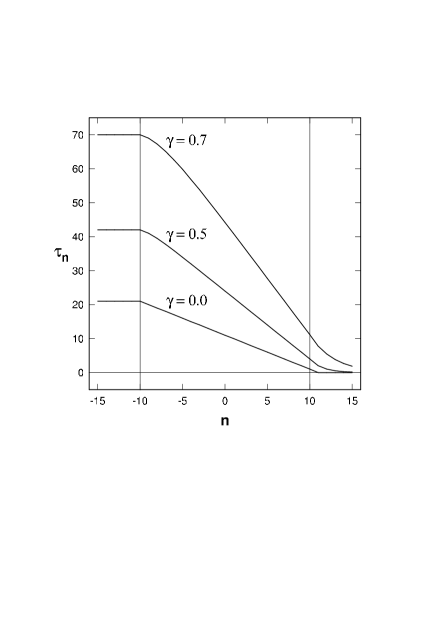
Figure 1: MRT for a nondisordered chain [as given by Eq. (22)] plotted against the discrete initial condition $n$, with $a=1$ and $L=10$. The solid lines are only to guide the eye.

where $\gamma=b/a<1$. Figure 1 shows the behavior of $\tau_{n}$ for some values of $\gamma$. We would like to stress that for $n<-L$, MRT is a constant proportional to the width of the interval ($2\,L+1$), whereas for $n\rightarrow\infty$, MRT vanishes. Given that the bias points to the right, for any initial condition at the left of the interval of interest, MRT is equal to the transit time across the interval. For a given initial condition, MRT is greater whereas the bias is smaller. For one way motion ($\gamma=0$), from Eq. (22) we obtain

$$\tau_{n}=\frac{1}{a}\left\{\begin{array}[]{ll}2\,L+1&,\;n<-L\\ L+1-n&,\;n\in D\\ 0&,\;n>L\,,\end{array}\right.$$ (23)

whereas in the small bias limit, i.e., $\gamma=1-\epsilon$, $\epsilon<<1$, taking $a$ constant results in

$$\tau_{n}=\frac{2\,L+1}{a\,\epsilon}\left\{\begin{array}[]{ll}1&\,,\,n<-L\\ \displaystyle 1-\frac{(L+n)\,(L+n+1)}{2\,(2\,L+1)}\,\epsilon&\,,\,n\in D\\ 1-n\,\epsilon&\,,\,n>L\,.\end{array}\right.$$ (24)

It is worthwhile to emphasize that MFPT exhibits a crossover from the drift (strong bias) regime [$T_{n}=(L+1-n)/a)$] to the diffusive (small bias) regime ($T_{n}\propto((L+1)^{2}-n^{2})/2a$). The diffusive behavior is also present for MRT for $n\in D$, but it is not in the leading term. Moreover, MFPT remains finite in the limit $\epsilon\rightarrow 0$ for finite domains, whereas MRT diverges as we can see from Eq. (24). Thus, the MRT is not a defined quantity for unbiased chains note:MRT . Expressions for the MFPT in nondisordered biased chains following from Eq. (21), and the study of the drift and diffusive regimes were reported in Ref. Pury94 .

V Projection Operator Average

The basic equation for the evolution of probabilities has been written in Eq. (13). The operators in this equation explicitly show the splitting of the transition probability in an average biased part ($\langle w_{n}^{+}\rangle=a$, $\langle w_{n}^{-}\rangle=b$) and a random nonbiased part ($\xi_{n}$). Defining the operator $\Delta=\xi_{n}\,{\cal K}^{0}$, let us rewrite Eq. (13) as

$$s\,\hat{F}(s)-F(0)=\left[{\cal K}^{b}+\Delta\right]\,\hat{F}(s)\;.$$ (25)

Our goal in this section is to obtain exact equations for the averaged survival and residence probabilities. This average can be formally carried out introducing a projection operator $\cal P$ (${\cal P}^{2}={\cal P}$) that averages over the joint probability density of variables $\{\xi_{n}\}$: $\langle\hat{F}\rangle\equiv{\cal P}\,\hat{F}$, $\hat{F}=\langle\hat{F}\rangle+(1-{\cal P})\,\hat{F}$. Applying the operator $\cal P$ to Eq. (25) we obtain

$$s\,\langle\hat{F}\rangle-F(0)={\cal K}^{b}\langle\hat{F}\rangle+{\cal P}\Delta\langle\hat{F}\rangle+{\cal P}\Delta(1-{\cal P})\hat{F}\;.$$ (26)

Also, applying the operator $(1-{\cal P})$ to Eq. (25) we arrive to

$$\begin{array}[]{rcl}s(1-{\cal P})\hat{F}&=&{\cal K}^{b}(1-{\cal P})\hat{F}+(1-{\cal P})\Delta\langle\hat{F}\rangle\\ &+&(1-{\cal P})\Delta(1-{\cal P})\hat{F}\;.\end{array}$$ (27)

A formal solution of Eq. (27) can be obtained using the Green’s function for the nondisordered chain,

$$\hat{G}(s)=\left(s-{\cal K}^{b}\right)^{-1}\;.$$ (28)

Applying $\hat{G}$ to Eq. (27) and using the definition given in Eq. (28), results in

$$(1-{\cal P})\hat{F}=\hat{G}\left[(1-{\cal P})\Delta\langle\hat{F}\rangle+(1-{\cal P})\Delta(1-{\cal P})\hat{F}\right]\;.$$ (29)

Equation (29) can be iteratively solved for $(1-{\cal P})\hat{F}$,

$$(1-{\cal P})\hat{F}=\sum_{k=1}^{\infty}\left[\hat{G}(1-{\cal P})\Delta\right]^{k}\langle\hat{F}\rangle\;.$$ (30)

Putting this formal solution in Eq. (26) we find a closed exact equation for the average probability $\langle\hat{F}\rangle$,

$$s\,\langle\hat{F}\rangle-F(0)={\cal K}^{b}\langle\hat{F}\rangle+\left\langle\sum_{k=0}^{\infty}\left[\Delta\hat{G}(1-{\cal P})\right]^{k}\Delta\right\rangle\langle\hat{F}\rangle\,.$$ (31)

The operator $\hat{G}$ is solution of the equation,

$$\left(s-{\cal K}^{b}\right)\hat{G}=\openone\,,$$ (32)

with the boundary conditions

$$\hat{G}^{S}_{-(L+1)\,m}(s)=\hat{G}^{S}_{(L+1)\,m}(s)=0\;\forall\,s\mbox{ and }m\in D\;,$$ (33a)

$$\hat{G}^{R}_{nm}(s)\rightarrow 0\;\mbox{ for }|n|\rightarrow\infty\mbox{ and }m\mbox{ finite}\;,$$ (33b)

where the superscript $S$ ($R$) corresponds to the survival (residence) problem. Exact expressions of the Green’s functions are calculated in the Appendix B.

We will find it useful to write Eq. (31) in components. For this task, we use the explicit form of $\Delta$, the Terwiel’s cumulants Terwiel of the random variables $\xi_{k}$: $\langle\xi_{n}\xi_{m_{1}}\ldots\xi_{m_{p}}\rangle_{T}={\cal P}\,\xi_{n}\,(1-{\cal P})\,\xi_{m_{1}}\dots(1-{\cal P})\,\xi_{m_{p}}$, and we define the propagator: $J_{nm}(s)={\cal K}^{0}\,\hat{G}_{nm}(s)$, where the operator ${\cal K}^{0}$ acts on the first index of $\hat{G}_{nm}(s)$. Explicit expressions for $J_{nm}(s)$ are given by Eqs. (LABEL:JS) and (LABEL:JR) in Appendix B. In this manner we can write

$$s\,\langle\hat{F}_{n}\rangle-F_{n}(0) = {\cal K}^{b}\langle\hat{F}_{n}\rangle\,+\,\sum_{p=0}^{\infty}\,\sum_{m_{1},\ldots,m_{p}}$$

$$\times\langle\xi_{n}\xi_{m_{1}}\ldots\xi_{m_{p}}\rangle_{T}\,J_{nm_{1}}(s)$$

$$\times J_{m_{1}m_{2}}(s)\ldots J_{m_{p-1}m_{p}}(s)\;{\cal K}^{0}\langle\hat{F}_{m_{p}}\rangle\,.$$

We must understand that $m_{0}=n$, and for the survival problem we have the additional restriction $m_{1},\ldots,m_{p}\in D$. The exact effective backward equation given by Eq. (LABEL:avF1) can be rewritten as

$$s\,\langle\hat{F}_{n}\rangle-F_{n}(0) = {\cal K}^{b}\langle\hat{F}_{n}\rangle\,+\,\sum_{p=0}^{\infty}\,\sum_{{{m_{1}\neq n\atop m_{2}\neq m_{1}}\atop\vdots}\atop m_{p}\neq m_{p-1}}$$

$$\times\langle\psi_{n}\psi_{m_{1}}\ldots\psi_{m_{p}}\rangle_{T}\;\,J_{nm_{1}}(s)$$

$$\times J_{m_{1}m_{2}}(s)\ldots J_{m_{p-1}m_{p}}(s)\;{\cal K}^{0}\,\langle\hat{F}_{m_{p}}\rangle\,,$$

where we have used the definition of Terwiel’s cumulants. Here, we have summed up all the terms containing the diagonal parts of $J_{nm}(s)$ through the introduction of the random operator $\psi_{k}(s)$ defined by

$$\psi_{k}(s)=\sum_{i_{k}=0}^{\infty}\,\left[J_{kk}(s)\,\xi_{k}(1-{\cal P})\right]^{i_{k}}\,\xi_{k}\,.$$ (36)

This operator acts on any disorder-dependent quantity at its right. The geometrical sum in Eq. (36) can be evaluated, resulting in

$$\psi_{k}(s)=M_{k}(s)-\frac{M_{k}(s)\,J_{kk}(s)}{1+\langle M_{k}(s)\rangle\,J_{kk}(s)}\,{\cal P}M_{k}(s)\,,$$ (37)

where

$$M_{k}(s)=\frac{\xi_{k}}{1-\xi_{k}\,J_{kk}(s)}\,.$$ (38)

In the following, we take the limit $s\rightarrow 0$ in order to obtain from Eq. (LABEL:avF2) the corresponding equations for the MFPT and MRT in disordered media, which are defined from Eq. (11) by

$$\left<T_{n}\right> = \lim_{s\rightarrow 0}\left<\hat{S}_{n}(s)\right>\;,$$ (39a)

$$\left<\tau_{n}\right> = \lim_{s\rightarrow 0}\left<\hat{R}_{n}(s)\right>\;.$$ (39b)

In this limit the propagator $J_{nm}(s)$ can be written as $\Lambda_{nm}+{\cal O}(s)$, and the exact expression for $\Lambda_{nm}$ in the FPT (RT) problem is given by Eq. (93) [Eq. (94)] in Appendix B. Therefore, the resulting equation for the averaged MFTP ($\langle T_{n}\rangle$) is

$$-S_{n}(t=0) = {\cal K}^{b}\langle T_{n}\rangle\,+\sum_{p=0}^{\infty}\,\sum_{{{m_{1}\neq n\atop m_{2}\neq m_{1}}\atop\vdots}\atop m_{p}\neq m_{p-1}}\langle\psi_{n}\psi_{m_{1}}\ldots\psi_{m_{p}}\rangle_{T}^{S}$$

$$\times\Lambda^{S}_{nm_{1}}\Lambda^{S}_{m_{1}m_{2}}\ldots\Lambda^{S}_{m_{p-1}m_{p}}\;{\cal K}^{0}\,\langle T_{m_{p}}\rangle\,.$$

Its solution must satisfy the boundary conditions: $\langle T_{-(L+1)}\rangle=\langle T_{L+1}\rangle=0$. A similar equation for the averaged MRT ($\langle\tau_{n}\rangle$) is obtained from Eq. (LABEL:avTeq) replacing the $S$ quantities by the corresponding $R$ quantities and imposing the boundary conditions: $\langle\tau_{n}\rangle=$ const for $n<-L$ and $\langle\tau_{n}\rangle\rightarrow 0$ for $n\rightarrow+\infty$ (given that the bias field points to right).

We, additionally, consider the case of small bias. Thus, the expressions for $\Lambda_{nm}$ can be further expanded, and taking $a$ constant results in

$$\Lambda^{S}_{nm}\approx\left\{\begin{array}[]{ll}\displaystyle\frac{1}{2\,(L+1)\,a}\,[m-(L+1)]\,\epsilon&,n<m\\ \displaystyle-\frac{1}{a}+\frac{1}{2\,(L+1)\,a}\,[m-(L+1)]\,\epsilon&,n=m\\ \displaystyle\frac{1}{2\,(L+1)\,a}\,[m+(L+1)]\,\epsilon&,n>m\;,\end{array}\right.$$ (41a)

$$\Lambda^{R}_{nm}\approx\frac{1}{a}\left\{\begin{array}[]{rl}0&,n<m\\ -1&,n=m\\ \epsilon&,n>m\;.\end{array}\right.$$ (41b)

Again, the superscript $S$ ($R$) corresponds to the survival (residence) problem. Hence, $\Lambda_{nm}\propto\epsilon$ for $n\neq m$ and, from Eq. (94), the diagonal components of the propagator in the residence problem result independent of $\epsilon$.

VI Weak Disorder

For disorder of class (a), the quantities $\beta_{k}$ are finite and we obtain that $\langle\psi_{n}\psi_{m_{1}}\ldots\psi_{m_{p}}\rangle_{T}^{S}\propto\epsilon^{0}$ and $\langle\psi_{n}\psi_{m_{1}}\ldots\psi_{m_{p}}\rangle_{T}^{R}$ is independent of $\epsilon$. Thus, Eq. (LABEL:avTeq) is a perturbative expansion in the sense that $\langle T_{n}\rangle$ can be calculated up to order $\epsilon^{q}$ truncating the $p$ series in the $q$ term ($p=0,\dots,q$). The corresponding equation for $\langle\tau_{n}\rangle$ is strictly a perturbative expansion given that the contribution to the order $\epsilon^{q}$ comes entirely from the term $p=q$.

In Eq. (LABEL:avTeq), the cumulant for $p=1$ consists of two independent random operators, so it vanishes (see Appendix C). Therefore, it turns out that only the term with $p=0$ contributes to order $\epsilon$. From Eq. (108) results

$$\langle\psi_{n}\rangle_{T}^{S}=\beta_{1}^{-1}-a-a\,{\cal F}\,\frac{L+1-n}{2\,(L+1)}\,\epsilon\;,$$ (42)

where we have introduced the fluctuation of the quenched disorder: ${\cal F}=(\beta_{2}-\beta_{1})/\beta_{1}^{2}$. Up to order $\epsilon$, taking $a$ constant and using ${\cal K}^{b}\approx a\left[{\cal K}^{0}-({\cal E}^{-}-{\cal I})\,\epsilon\right]$, the explicit form of Eq. (LABEL:avTeq) is

$$-1 = \beta_{1}^{-1}\,{\cal K}^{0}\,\langle T_{n}\rangle$$

$$-a\left[{\cal F}\,\frac{L+1-n}{2\,(L+1)}\,{\cal K}^{0}+({\cal E}^{-}-{\cal I})\right]\epsilon\,\langle T_{n}\rangle+{\cal O}(\epsilon^{2})\,.$$

For $\epsilon=0$, Eq. (LABEL:MFPTeq) immediately gives the well-known MFPT for the unbiased case: $\langle T_{n}(\epsilon=0)\rangle=\left[(L+1)^{2}-n^{2}\right]/\left(2\,\beta_{1}^{-1}\right)$, where we can see that the effect of weak disorder is to replace the constant $a$ by the effective coefficient $\beta_{1}^{-1}$. To construct the consistent solution up to order $\epsilon$ of Eq. (LABEL:MFPTeq), we propose the expression

$$\langle T_{n}\rangle=\frac{(L+1)^{2}-n^{2}}{2\,\beta_{1}^{-1}}\left[1+(A\,n+B)\,\epsilon\right]\,,$$ (44)

which immediately satisfies the boundary conditions: $\langle T_{-(L+1)}\rangle=\langle T_{L+1}\rangle=0$. To fit the constants $A$ and $B$ we substitute this expression in Eq. (LABEL:MFPTeq) and retain only the terms up to order $\epsilon$. If the factor of $\epsilon$ in the expression (44) were a polynomial of degree greater than $1$, we can easily see that the coefficients of the terms of degree greater than $1$ vanish. Thus, we obtain for $n\in D$

$$\langle T_{n}\rangle \approx \frac{(L+1)^{2}-n^{2}}{2\,\beta_{1}^{-1}}$$

$$\times\left[1+\left(\frac{3-2n}{6}+\frac{L+1-n/3}{2\,(L+1)}\,{\cal F}\right)a\beta_{1}\,\epsilon\right].$$

From this expression we can analyze the interplay between the bias and the fluctuation of the quenched disorder ${\cal F}$. In the presence of bias, the escape time from the finite interval increases for all initial conditions $n$, with respect to the unbiased case, if the fluctuation is large enough. This is an important result related to the control of the trapping process. This fact was reported in Ref. Pury94 where the solution of Eq. (LABEL:MFPTeq) was constructed from FEMA. Now, we can evaluate the difference between the exact solution (order $\epsilon$) given by Eq. (LABEL:MFPT) and that approximation, obtaining that the correction to FEMA is $\frac{(L+1)^{2}-n^{2}}{6\,(L+1)}\,n\,{\cal F}\,a\,\epsilon$.

In the residence problem, from Eqs. (103) and (108) results $\langle\psi_{n}\rangle_{T}^{R}=\beta_{1}^{-1}-a$. Thus, the corresponding equation for the averaged MRT is

$$-R_{n}(0)=\beta_{1}^{-1}\,{\cal K}^{0}\,\langle\tau_{n}\rangle-a\,\epsilon\,({\cal E}^{-}-{\cal I})\,\langle\tau_{n}\rangle+{\cal O}(\epsilon^{2})\,,$$ (46)

where $R_{n}(0)$ is given by Eq. (16). Now we have to deal with a backward master equation with constant coefficients. In this case, the fluctuations of disorder are not present. Formally, this equation is equal to the one corresponding to a nondisordered chain in the small limit bias. Therefore, from Eq. (24), with the substitutions

$$a \rightarrow \beta_{1}^{-1}\,,$$

$$b \rightarrow \beta_{1}^{-1}(1-a\,\beta_{1}\,\epsilon)\,,$$

$$\epsilon \rightarrow a\,\beta_{1}\,\epsilon\,,$$ (47)

we obtain, up to order $\epsilon$, the solution

$$\tau_{n}\approx\frac{2\,L+1}{a\,\epsilon}\left\{\begin{array}[]{ll}1&,n<-L\\ \displaystyle 1-\frac{(L+n)\,(L+n+1)}{2\,(2\,L+1)}a\beta_{1}\epsilon&,n\in D\\ 1-n\,a\,\beta_{1}\,\epsilon&,n>L\;.\end{array}\right.$$ (48)

VII Strong Disorder

For the classes of strong disorder, $\beta_{k}$ are divergent quantities in the limit $\epsilon\rightarrow 0$,

$$\begin{array}[]{ll}\beta_{1}\approx|\ln\epsilon|/(2a)&\\ \beta_{k}\approx\displaystyle\frac{(a\epsilon)^{1-k}}{2a(k-1)}&(k>1)\end{array},\;\mbox{for class (\ref{windows})},$$ (49a)

$$\beta_{k}\approx\frac{C}{k-1+\alpha}(a\epsilon)^{1-k-\alpha},\;\mbox{for class (\ref{alpha})},$$ (49b)

where $0<\alpha<1$ and $C$ is given in Eq. (20b). Also in this limit, Terwiel’s cumulants diverge except the first one, $\langle\psi_{n}\rangle_{T}$, which vanishes. However, all the terms of the $p$ series in the Eq. (LABEL:avTeq) vanish and the one corresponding to $p=0$ is the leading term. We reckon the relevant cumulants in Appendix C.

For a disorder of class (18) we obtain ${\cal F}\approx\frac{2}{\epsilon\,\ln^{2}\epsilon}$, and from Eq.(42) results $\langle\psi_{n}\rangle_{T}^{S}\approx\beta_{1}^{-1}$. Therefore, the leading terms in the equation for the averaged MFPT result in

$$-1=\beta_{1}^{-1}\,{\cal K}^{0}\,\langle T_{n}\rangle+{\cal O}\left(\frac{\epsilon}{|\ln\epsilon|}\right)\,.$$ (50)

This is a backward master equation for the unbiased chain with constant coefficients whose solution is given by $\langle T_{n}\rangle=\left[(L+1)^{2}-n^{2}\right]/\left(2\,\beta_{1}^{-1}\right)$. Hence, the averaged MFPT diverges as $\beta_{1}\propto|\ln\epsilon|$.

On the other hand, for a disorder of class (20) we obtain ${\cal F}\approx\frac{1}{C}\frac{\alpha^{2}}{1+\alpha}(a\,\epsilon)^{\alpha-1}$, and from Eq. (42) results $\langle\psi_{n}\rangle_{T}^{S}\approx\beta_{1}^{-1}\left(1-\frac{\alpha}{1+\alpha}\,\frac{L+1-n}{2\,(L+1)}\right)$. Therefore, the MFPT’s equation is

$$-1=\left(1-\frac{\alpha}{1+\alpha}\,\frac{L+1-n}{2\,(L+1)}\right)\beta_{1}^{-1}\,{\cal K}^{0}\,\langle T_{n}\rangle+{\cal O}(\epsilon)\,.$$ (51)

In this case, we get an unbiased backward master equation with linear coefficients. General solutions of this equation will be given elsewhere. Nevertheless, we hold our attention in the divergent behavior of the averaged MFPT for $\epsilon\rightarrow 0$. From Eq. (51) we can see that $\langle T_{n}\rangle\propto\beta_{1}\propto\epsilon^{-\alpha}$.

FEMA Pury94 consists in introducing an effective nonhomogeneous medium $\Gamma_{n}$ and truncating Eq. (LABEL:avTeq) to the first term: $-1={\cal K}^{b}\langle T_{n}\rangle$. Here, the operator ${\cal K}^{b}$ is constructed with the constants $a+\Gamma_{n}$ and $b+\Gamma_{n}$. The effective rate, $\Gamma_{n}$, is fixed imposing the condition $\langle\psi_{n}(\Gamma_{n})\rangle_{T}^{S}=0$. The resulting solutions give the exact laws: $\langle T_{n}\rangle\propto|\ln\epsilon|$, for a disorder of class (18) and $\langle T_{n}\rangle\propto\epsilon^{-\alpha}$, for a disorder of class (20), however in the last case the predicted $n$-dependent coefficient is not exact. Strikingly, the predicted divergence laws for the averaged MFPT in biased chains agree with the corresponding laws for the survival probability, obtained for the unbiased case in the limit $s\rightarrow 0$ HC90 . The behavior of the survival probability obtained from FEMA is $\langle\hat{S}_{n}(s)\rangle\propto|\ln s|$, for a disorder of class (18), and $\langle\hat{S}_{n}(s)\rangle\propto s^{-\alpha}$, for a disorder of class (20). Accordingly, both problems have the same exponents despite their different nature.

In the residence problem, for both classes of strong disorder we get that $\langle\psi_{n}\rangle_{T}^{R}\approx\beta_{1}^{-1}$, and then the equation for the averaged MRT results $-R_{n}(0)=\beta_{1}^{-1}\,{\cal K}^{0}\,\langle\tau_{n}\rangle$, i.e., an unbiased equation. Therefore, the averaged MRT is not a defined quantity for strong disorder.

VIII Thermally Activated Processes

Before concluding this work, we want to analyze the physical realization corresponding to thermally activated processes in weakly disordered chains. For this goal we suppose a particle that moves in a periodic potential $U$ with minima separated by sharp maxima of height $\phi$.The jump probability per unit time to neighbor sites involves the Arrhenius factor: $W\exp(-\beta\,\phi)$ with $\beta=(k_{B}T)^{-1}$, where $k_{B}$ is Boltzmann’s constant and $T$ is the temperature.

Figure 2: Disordered potential in the chain. $d$ is the distance between nearest-neighbor sites. The particle jumps to neighboring sites through potential barriers equal to $\phi-\phi_{n}$, where $\phi_{n}$ are independent identically distributed random variables with zero mean.

In the presence of disorder, the transition probabilities are still symmetrical but depend on the site [see Fig. (2)]: $w_{n}=W\exp[-\beta(\phi-\phi_{n})]$, where $\langle\phi_{n}\rangle=0$, $|\phi_{n}|\ll\phi$, and we suppose that the random potential is smaller than the thermal energy, i.e., $\beta|\phi_{n}|\ll 1$. Now, suppose that an external field $E$ (toward right) is added, then the force $q\,E$ is applied on the particle of “charge” $q$. The presence of $E$ alters the heights of potential barriers. The new jump probabilities are nonsymmetric,

$$w_{n}^{\pm}=W\exp[-\beta(\phi-\phi_{n}\mp q\,E\,d/2)]\,,$$ (52)

where $d$ is the separation between neighbor sites. In the low field limit, we can use the aproximation $\exp[-\beta(-\phi_{n}\mp q\,E\,d/2)]\approx 1+\beta\,\phi_{n}\pm\beta\,q\,E\,d/2$, thus [see Eq. (12)],

$$a = W\exp(-\beta\,\phi)\left(1+\beta\,q\,E\,d/2\right)\,,$$ (53a)

$$b = W\exp(-\beta\,\phi)\left(1-\beta\,q\,E\,d/2\right)\,,$$ (53b)

$$\xi_{n} = W\exp(-\beta\,\phi)\,\beta\,\phi_{n}\,.$$ (53c)

Hence, $\gamma=b/a\approx 1-\beta\,q\,E\,d$, i.e., $\epsilon=\beta\,q\,E\,d$.

Defining $a_{0}=W\exp(-\beta\,\phi)$, we can write $a=a_{0}(1+\epsilon/2)$, $b=a_{0}(1-\epsilon/2)$, and $\xi_{n}=a_{0}\beta\phi_{n}$. Therefore, we must adapt the equations of Sec. VI to incorporate the lineal dependence of $a$ on $\epsilon$. In the following, it will be useful to define the quantities $\overline{w}=a_{0}+\xi_{n}$, $\overline{\beta_{k}}=\left<\overline{w}^{-k}\right>$, and $\overline{\cal F}=\overline{\beta_{2}}/\overline{\beta_{1}}^{2}-1$ which are independent of $\epsilon$. From Eqs. (93) and Eqs. (94) results that Eqs. (41b) are valid with the substitution $a\rightarrow a_{0}$. Additionally, we can see that $\langle\psi_{n}\rangle_{T}=\overline{\beta}_{1}^{-1}-a_{0}-a_{0}\,\overline{\cal F}\,\theta_{n}\,\epsilon$, where $\theta_{n}$ is given by Eq. (103). Now, using that ${\cal K}^{b}\approx a_{0}\left[{\cal K}^{0}-({\cal E}^{+}-{\cal E}^{-})\,\epsilon/2\right]$, the explicit form of the MFPT’s equation up to order $\epsilon$ is

$$-1=\overline{\beta}_{1}^{-1}\,{\cal K}^{0}\,\langle T_{n}\rangle-a_{0}\left[\overline{\cal F}\,\theta_{n}\,{\cal K}^{0}+\frac{1}{2}\,({\cal E}^{+}-{\cal E}^{-})\right]\epsilon\,\langle T_{n}\rangle\,.$$ (54)

Proposing the solution given by Eq.(44), we now obtain

$$\langle T_{n}\rangle \approx \frac{(L+1)^{2}-n^{2}}{2\,\overline{\beta}_{1}^{-1}}$$

$$\times\left[1+\left(-\frac{n}{3}+\frac{L+1-n/3}{2\,(L+1)}\,\overline{\cal F}\right)a_{0}\overline{\beta}_{1}\,\epsilon\right].$$

In order to obtain the explicit dependence on temperature, we additionally must replace the disorder-dependent quantities according to $\overline{\beta}_{1}\approx(1+\beta^{2}\langle\phi_{n}^{2}\rangle)/a_{0}$ and $\overline{\cal F}\approx\beta^{2}\langle\phi_{n}^{2}\rangle$.

On the other hand, the MRT’s equation up to order $\epsilon$ results

$$-R_{n}(0)=\overline{\beta}_{1}^{-1}\,{\cal K}^{0}\,\langle\tau_{n}\rangle+\frac{a_{0}}{2}\,\epsilon\,({\cal E}^{+}-{\cal E}^{-})\,\langle\tau_{n}\rangle\;.$$ (56)

Again, this equation is equal to that corresponding to a nondisordered chain for small bias with transition rates given by the substitutions

$$a \rightarrow \overline{\beta}_{1}^{-1}+\frac{a_{0}}{2}\,\epsilon,$$

$$b \rightarrow \overline{\beta}_{1}^{-1}-\frac{a_{0}}{2}\,\epsilon,$$

$$\epsilon \rightarrow a_{0}\,\overline{\beta}_{1}\,\epsilon\,,$$ (57)

Thus, up to order $\epsilon$, MRT is equal to the expression given by Eq. (48) with the changes $a\rightarrow a_{0}$ and $\beta_{1}\rightarrow\overline{\beta}_{1}$.

IX Conclusions

We have presented a unified framework for the FPT and RT statistics in finite disordered chains with bias. Exact equations for the quantities averaged over disorder were obtained for both problems and its solutions up to first order in the bias parameter were constructed retaining the full dependence on the system’s size and the initial condition.

We have studied the FPT and RT problems for three models of disorder. For weak disorder, the inverse moments of the transition probabilities are finite, and we get that the bias becomes a control parameter for the MFPT, coupled with the fluctuation of the disorder. The MRT is only defined in the presence of bias, and for weak disorder the MRT’s expressions are obtained from the nondisordered case renormalizing the transition constants. For strong disordered cases, for which the MFPT is not defined in unbiased chains, the bias allows us to study the divergent behavior. Amazingly, the exponents of the divergences in MFPT obtained for vanishing bias coincide with that obtained for the averaged survival probability in the long time regime. The MRT is a divergent quantity under strong disorder because the strength parameter is not present in the corresponding equation in the small bias limit, and the MRT is not defined for unbiased walks.

We complete the work with three appendixes. In Appendix A the derivation of survival and residence probabilities for nondisordered chains is completely developed. Apppendix B is devoted to the detailed calculation of Green’s function in a chain with bias. Exact expressions are given, which display the full dependence on the system’s size, initial condition, and bias strength. The evaluation of the relevant Terwiel’s cumulants is reported in Appendix C.

Appendix A Survival and Residence Probabilities in a nondisordered biased chain

We address the question about the survival and residence probabilities for a RW in the finite interval $\bar{D}=[-M,L]$ of a homogeneous chain. In the absence of disorder, the Laplace transform of the evolution equation gives $s\hat{F}_{n}(s)-F_{n}(0)={\cal K}^{b}\hat{F}_{n}(s)$. This equation can be written as

$$\left[a\;{\cal E}^{+}+b\;{\cal E}^{-}-(s+a+b)\;{\cal I}\right]\hat{F}_{n}(s)=-F_{n}(0)\;,$$ (58)

and must be solved with the boundary conditions corresponding to each problem,

$$\hat{S}_{-(M+1)}(s)=\hat{S}_{(L+1)}(s)=0\,,$$ (59a)

$$\hat{R}_{n}(s)\rightarrow 0\mbox{ for }|n|\rightarrow\infty\,,$$ (59b)

$\forall s>0$. Defining the vector $A$ such that $A_{n+1}\equiv\hat{F}_{n}(s)$, Eq. (58) can be written as

$$\left(a\;({\cal E}^{+})^{2}-(s+a+b)\;{\cal E}^{+}+b\;{\cal I}\right)A_{n}=-F_{n}(0)\;.$$ (60)

Equation (60) is a second-order linear difference equation. A particular solution for the inhomogeneous equation is the constant $A_{n}=1/s$. Proposing $A_{n}=x^{n}$ as a solution of the corresponding homogeneous equation, it gives $x^{2}-(r+1+\gamma)\,x+\gamma=0$, where $r=s/a$ and $\gamma=b/a<1$. The roots of this second-order equation are given by

$$x_{1,2}=\frac{1}{2}\left[r+1+\gamma\pm\sqrt{(r+1+\gamma)^{2}-4\,\gamma}\right]$$ (61)

and satisfy $x_{1}\,x_{2}=\gamma$ with $x_{1}\geq 1$. Then, the general solution of Eq. (58) can be written as

$$\hat{F}_{n}(s)=\frac{1}{s}+c_{1}\,x_{1}^{n}+c_{2}\,x_{2}^{n}\;,\;\;n\in\bar{D}\,.$$ (62)

For the survival problem the constants $c_{1}$ and $c_{2}$ are fixed by imposing the boundary conditions given by Eq. (59a). Thus, we found for the survival probability the following expression:

$$\hat{S}_{n}(s)=\frac{1}{s}\left(1-\frac{\left(x_{1}^{L+M+2}-\gamma^{L+M+2}\right)\,x_{1}^{n-L-1}+\left(\gamma^{L+M+2}-x_{2}^{L+M+2}\right)\,x_{2}^{n-L-1}}{x_{1}^{L+M+2}-x_{2}^{L+M+2}}\right)\;.$$ (63)

This equation is invariant under the transformation $x_{1}\leftrightarrow x_{2}$. From Eq. (63) and $\hat{f}_{n}(s)=1-s\,\hat{S}_{n}(s)$, we can immediately obtain the FPTD for the ordered chain.

For the residence problem, the boundary conditions (59b) impose that

$$\hat{R}_{n}(s)=\left\{\begin{array}[]{ll}d_{1}\,x_{1}^{n}&\mbox{for $n<-M$}\\ d_{2}\,x_{2}^{n}&\mbox{for $n>L$}\;.\end{array}\right.$$ (64)

Now, the constants $c_{1}$, $c_{2}$, $d_{1}$, and $d_{2}$ are fixed by writing explicitly Eq. (58) for the sites $n=-(M+1)$, $-M$, $L$, and $L+1$. Thus, we finally found the expression for the residence probability,

$$\hat{R}_{n}(s)=\frac{1}{s\,(x_{1}-x_{2})}$$

$$\times\left\{\begin{array}[]{l}(1-x_{2})\,\left(x_{1}^{L+M+1}-1\right)\,x_{1}^{n-L}\,,\;n<-M\\ 1-\left[(1-x_{2})\,x_{1}^{n-L}+(x_{1}-1)\,x_{2}^{M+1+n}\right],\;n\in D\\ (x_{1}-1)\left(1-x_{2}^{L+M+1}\right)\,x_{2}^{n-L}\,\;n>L\;.\end{array}\right.$$ (68)

(69)

Taking the limits of Eq. (11) it gives, on one hand the MFPT for the ordered chain,

$$T_{n}=\frac{L+1-n}{a(1-\gamma)}-\frac{L+M+2}{a(1-\gamma)}\,\frac{\gamma^{n}-\gamma^{L+1}}{\gamma^{-(M+1)}-\gamma^{L+1}}\;,$$ (70)

with $-M\leq n\leq L$, and on the other hand the MRT,

$$\tau_{n}=\frac{1}{a}\left\{\begin{array}[]{ll}\displaystyle\frac{L+M+1}{1-\gamma}&,\;n<-M\\ \displaystyle\frac{L-n}{1-\gamma}+\frac{1-\gamma^{n+M+1}}{(1-\gamma)^{2}}&,\;-M\leq n\leq L\\ \displaystyle\frac{1-\gamma^{L+M+1}}{(1-\gamma)^{2}}\;\gamma^{n-L}&,\;n>L\;.\end{array}\right.$$ (71)

Equations (21) and (22) follow from Eqs. (70) and and (71), respectively, taking $M=L$.

Appendix B Green’s Function in a chain with Bias

In this section we are concerned with the solution of Eq. (32). In components, this backward equation can be written as

$$a\,\hat{G}_{n+1m}(s)+b\,\hat{G}_{n-1m}(s)-(s+a+b)\,\hat{G}_{nm}(s)=-\delta_{nm}.$$ (72)

We must solve this equation with the boundary conditions corresponding to each problem,

$$\hat{G}^{S}_{-(M+1)\,m}(s)=\hat{G}^{S}_{(L+1)\,m}(s)=0\;\forall\,s\mbox{ and }m\in\bar{D}\;,$$ (73a)

$$\hat{G}^{R}_{nm}(s)\rightarrow 0\;\mbox{ for }|n|\rightarrow\infty\mbox{ and }m\mbox{ finite}\;.$$ (73b)

Here, the superscript $S$ ($R$) denotes the solution corresponding to the survival (residence) problem.

The solution of Eq. (72) in a finite domain (survival problem) can be constructed using the method of images MW87 . It consists in summing to the Green’s function in the absence of boundaries, terms corresponding to the specular image of the index $n$ with respect to the boundary considered. For absorbing boundaries the image must have a negative sign. Moreover, in the presence of bias, the image must change the bias direction ($a\leftrightarrow b$). Additionally, in a closed domain, each boundary reflects the image of the other boundary. This fact introduces an infinite set of images. However, we adopt here the simpler algebraic approach developed in Appendix A. Thus, we propose

$$\hat{G}^{S}_{nm}(s)=\left\{\begin{array}[]{ll}\gamma_{1}\,x_{1}^{n}+\gamma_{2}\,x_{2}^{n}&\mbox{for $n\leq m$}\\ \delta_{1}\,x_{1}^{n}+\delta_{2}\,x_{2}^{n}&\mbox{for $n\geq m$}\end{array}\right.\mbox{ with }n,m\,\in\bar{D}\;,$$ (74)

where the functions $x_{1,2}$ are defined in Eq. (61). The constants $\gamma_{1}$, $\gamma_{2}$, $\delta_{1}$, and $\delta_{2}$ are solutions of the set of four algebraic equations that result from imposing the boundary conditions given by Eq. (73a), imposing the equality between both expressions given by Eq. (74) for $n=m$, and writing Eq. (72) for $n=m$. Additionally, using the relation $a\,x_{1,2}^{2}-(s+a+b)\,x_{1,2}+b=0$ we obtain

$$\hat{G}^{S}_{nm}(s)=\frac{1}{D}\,\left\{\begin{array}[]{ll}x_{1}^{n+M+1}\left(x_{1}^{-m+L+1}-x_{2}^{-m+L+1}\right)+x_{2}^{n+M+1}\left(x_{2}^{-m+L+1}-x_{1}^{-m+L+1}\right)&,n\leq m\\ x_{1}^{n}\,x_{2}^{L+1}\left(x_{1}^{-m}x_{2}^{M+1}-x_{2}^{-m}x_{1}^{M+1}\right)+x_{2}^{n}\,x_{1}^{L+1}\left(x_{2}^{-m}x_{1}^{M+1}-x_{1}^{-m}x_{2}^{M+1}\right)&,n\geq m\;,\end{array}\right.$$ (75)

where $D=a\,(x_{1}-x_{2})\,\left(x_{1}^{L+M+2}-x_{2}^{L+M+2}\right)$. Defining the variable $z=s+a+b-2\,\mu$, the constant $\mu=\sqrt{ab}$, and the functions

$$A(z)=1+\frac{z}{2\mu}-\left(\frac{z}{\mu}+\frac{z^{2}}{4\mu^{2}}\right)^{1/2}\;,$$ (76a)

$$B(z)=\frac{1}{2\mu}\,\left(\frac{z}{\mu}+\frac{z^{2}}{4\mu^{2}}\right)^{-1/2}\;,$$ (76b)

results in $x_{2}=\sqrt{\gamma}\,A(z)$ and $a(x_{1}-x_{2})=B(z)^{-1}$. Using these functions we can recast the expression (75), for the case $M=L$, as

$$\hat{G}^{S}_{nm}(s) = \gamma^{\frac{n-m}{2}}\,B(z)\,\left[1-A(z)^{4\,(L+1)}\right]^{-1}$$ (77)

$$\times\left[\rule{0.0pt}{11.38109pt}\right.A(z)^{|n-m|}$$

$$-A(z)^{2\,(L+1)}\left(A(z)^{n+m}+A(z)^{-(n+m)}\right)$$

$$\left.+A(z)^{4\,(L+1)}\,A(z)^{-|n-m|}\right]\;.$$

The last expression satisfies the symmetry relation $(a,b),(n,m)\leftrightarrow(b,a),(m,n)$. Denoting by $\hat{\cal G}^{S}_{nm}(s)$ the Green’s function corresponding to the survival problem without bias (and taking $\mu=\sqrt{ab}$) HC90 , we can immediately see that $\hat{G}^{S}_{nm}(s)=\gamma^{\frac{n-m}{2}}\,\hat{\cal G}^{S}_{nm}(z)$. Moreover, given that $\left(z-\mu\,{\cal K}^{0}\right)\hat{\cal G}^{S}(z)=\openone$, we immediately obtain Eq. (72).

We now compute the propagator $J_{nm}(s)={\cal K}^{0}\hat{G}_{nm}(s)$. Applying the operator ${\cal K}^{0}$ defined in Eq. (14) to Eq. (77), the following expression is found:

$$J^{S}_{nm}(s) = B(z)\,\left[1-A(z)^{4\,(L+1)}\right]^{-1}\left[\rule{0.0pt}{14.22636pt}\right.-A(z)^{2\,(L+1)}$$

$$\times\left\{\left(\frac{\sqrt{\gamma}}{A(z)}\right)^{n}\,\left[\sqrt{\gamma}\,A(z)\right]^{-m}\left(\frac{\sqrt{\gamma}}{A(z)}+\frac{A(z)}{\sqrt{\gamma}}-2\right)\right.$$

$$+\left.\left[\sqrt{\gamma}\,A(z)\right]^{n}\,\left(\frac{A(z)}{\sqrt{\gamma}}\right)^{m}\left(\sqrt{\gamma}\,A(z)+\frac{1}{\sqrt{\gamma}\,A(z)}-2\right)\right\}+{\cal Z}_{nm}\;\left.\rule{0.0pt}{14.22636pt}\right]\;,$$

where $n,m\,\in D$ and

$${\cal Z}_{nm}=\left\{\begin{array}[]{ll}\displaystyle\left(\frac{\sqrt{\gamma}}{A(z)}\right)^{n-m-1}\,\left(\frac{\sqrt{\gamma}}{A(z)}-1\right)^{2}+A(z)^{4\,(L+1)}\,\left(\sqrt{\gamma}\,A(z)\right)^{n-m-1}\,\left(\sqrt{\gamma}\,A(z)-1\right)^{2}&,n<m\\ \displaystyle\sqrt{\gamma}\,A(z)+\frac{A(z)}{\sqrt{\gamma}}-2+A(z)^{4\,(L+1)}\,\left(\frac{\sqrt{\gamma}}{A(z)}+\frac{1}{\sqrt{\gamma}\,A(z)}-2\right)&,n=m\\ \displaystyle\left(\sqrt{\gamma}\,A(z)\right)^{n-m-1}\,\left(\sqrt{\gamma}\,A(z)-1\right)^{2}+A(z)^{4\,(L+1)}\,\left(\frac{\sqrt{\gamma}}{A(z)}\right)^{n-m-1}\,\left(\frac{\sqrt{\gamma}}{A(z)}-1\right)^{2}&,n>m\;.\end{array}\right.$$ (79)

On the other hand, for the residence problem we propose

$$\hat{G}^{R}_{nm}(s)=\left\{\begin{array}[]{ll}\lambda_{1}\,x_{1}^{n}&\mbox{for $n\leq m$}\\ \lambda_{2}\,x_{2}^{n}&\mbox{for $n\geq m$}\end{array}\right.\mbox{ with }n,m\,\in\bar{D}\;.$$ (80)

This expression immediately satisfies the homogeneous case of Eq. (72) and the boundary conditions (73b), given that $x_{1}\,x_{2}=\gamma<1$ with $x_{1}\geq 1$. The constants $\lambda_{1}$ and $\lambda_{2}$ are fixed by imposing for $n=m$, the equality between both expressions in Eq. (80), and writting Eq. (72) for $n=m$. Hence, we obtain

$$\hat{G}^{R}_{nm}(s)=\frac{1}{a\,(x_{1}-x_{2})}\,\left\{\begin{array}[]{ll}\gamma^{n-m}\,x_{2}^{m-n}&\mbox{for }n\leq m\\ x_{2}^{n-m}&\mbox{for }n\geq m\;.\end{array}\right.$$ (81)

Using the functions defined by Eq. (76b), the last expression can be recast as

$$\hat{G}^{R}_{nm}(s)=\gamma^{(n-m)/2}\,B(z)\,A(z)^{|n-m|}\;.$$ (82)

Applying the operator ${\cal K}^{0}$ to Eq. (82) we find:

$$J^{R}_{nm}(s) = \gamma^{(n-m)/2}\,B(z)\;A(z)^{|n-m|}$$ (86)

$$\times\left\{\begin{array}[]{ll}\gamma^{1/2}\,A(z)^{-1}+\gamma^{-1/2}\,A(z)-2&,n<m\\ \gamma^{1/2}\,A(z)+\gamma^{-1/2}\,A(z)-2&,n=m\\ \gamma^{1/2}\,A(z)+\gamma^{-1/2}\,A(z)^{-1}-2&,n>m.\end{array}\right.$$

We are interested in analyzing the propagator $J_{nm}(s)$ in the limit $s\rightarrow 0$ for a given bias, also we are concerned with the expansion for small bias ($\epsilon\rightarrow 0$). We must stress that these limits do not commute. Thus, we first must take the limit $s\rightarrow 0$ for a fixed bias, and then perform the expansion in the parameter $\epsilon$. Defining the variable $y=s/(a-b)$, we get from Eq. (76b), for small $s$, that

$$A(z)\approx\sqrt{\gamma}\left(1-y+\frac{1}{1-\gamma}\,y^{2}\right)\,,$$ (88a)

$$B(z)\approx\frac{1}{a\,(1-\gamma)}\left(1-\frac{1+\gamma}{1-\gamma}\,y+\frac{(1+\gamma)^{2}+2\gamma}{(1-\gamma)^{2}}\,y^{2}\right)\,.$$ (88b)

These approximations allow us to write the propagator in the form: $J_{nm}(s)\approx\Lambda_{nm}+{\cal O}(y)$, where for the survival problem

$$\Lambda^{S}_{nm}=\frac{1}{a\,(1-\gamma)}\,\left(1-\gamma^{2\,(L+1)}\right)^{-1}$$

$$\times\left\{\begin{array}[]{ll}(1-\gamma^{2})\,\left(-\gamma^{n+L}+\gamma^{n-m+2L+1}\right)&,n<m\\ -(1-\gamma^{2})\,\gamma^{n+L}+(1-\gamma)\left(\gamma^{2L+1}-1\right)&,n=m\\ (1-\gamma^{2})\,\left(-\gamma^{n+L}+\gamma^{n-m-1}\right)&,n>m,\end{array}\right.$$ (92)

(93)

and, on the other hand, for the residence problem

$$\Lambda^{R}_{nm}=\frac{1}{a}\left\{\begin{array}[]{ll}0&,n<m\\ -1&,n=m\\ (1-\gamma)\,\gamma^{n-m-1}&,n>m\;.\end{array}\right.$$ (94)

We remark that we keep the exact dependence in the parameter $L$ (size of the system) for the FPT problem. From Eq. (93), we can also see that the $s$-independent contribution is quite different from that which is obtained without bias HC90 . In the presence of bias we get nondiagonal contributions to the propagator for the survival and residence problems in the limit $s\rightarrow 0$, which also remain for small bias, as has been shown in Eq. (41b).

Appendix C Terwiel’s Cumulants

The Terwiel’s cumulants were introduced in Ref. Terwiel . In this Appendix we are concerned with the evaluation of the cumulants of the random operator $\psi_{n}$ defined by

$$\psi_{n}=M_{n}\left(1-N_{n}\,{\cal P}M_{n}\right)\,,$$ (95)

where

$$M_{n}=\frac{\xi_{n}}{1-\xi_{n}\,J_{nn}}$$ (96)

is a random variable, and

$$N_{n}=\frac{J_{nn}}{1-\langle M_{n}\rangle\,J_{nn}}\,.$$ (97)

From its definition,

$$\langle\psi_{n}\psi_{m_{1}}\ldots\psi_{m_{p}}\rangle_{T}={\cal P}\,\psi_{n}\,(1-{\cal P})\,\psi_{m_{1}}\dots(1-{\cal P})\,\psi_{m_{p}}$$ (98)

can be easily obtained

$$\langle\psi_{n}\rangle_{T} = \langle\psi_{n}\rangle\,,$$

$$\langle\psi_{n}\psi_{m}\rangle_{T} = \langle\psi_{n}\psi_{m}\rangle-\langle\psi_{n}\rangle\langle\psi_{m}\rangle\,,$$

$$\langle\psi_{n}\psi_{m_{1}}\psi_{m_{2}}\rangle_{T} = \langle\psi_{n}\psi_{m_{1}}\psi_{m_{2}}\rangle-\langle\psi_{n}\rangle\langle\psi_{m_{1}}\psi_{m_{2}}\rangle$$

$$-\langle\psi_{n}\psi_{m_{1}}\rangle\langle\psi_{m_{2}}\rangle+\langle\psi_{n}\rangle\langle\psi_{m_{1}}\rangle\langle\psi_{m_{2}}\rangle\,.$$

For $n\neq m$, $\psi_{n}$ and $\psi_{m}$ are statistically independent, then $\langle\psi_{n}\psi_{m}\rangle=\langle\psi_{n}\rangle\langle\psi_{m}\rangle$. Therefore,

$$\langle\psi_{n}\psi_{m}\rangle_{T} = 0\,,$$

$$\langle\psi_{n}\psi_{m}\psi_{n^{\prime}}\rangle_{T} = 0\;\;(n\neq n^{\prime})\,,$$

$$\langle\psi_{n}\psi_{m}\psi_{n}\rangle_{T} = \langle\psi_{n}\psi_{m}\psi_{n}\rangle+\langle\psi_{n}\rangle\langle\psi_{m}\rangle\langle\psi_{n}\rangle\,,$$ (100)

and using Eqs. (95)-(97) results

$$\langle\psi_{n}\rangle = \frac{\langle M_{n}\rangle}{1+\langle M_{n}\rangle\,J_{nn}}\,,$$

$$\langle\psi_{n}\psi_{m}\psi_{n}\rangle_{T} = \left(1+\langle M_{n}\rangle\,J_{nn}\right)^{-2}$$

$$\times\left(\langle M_{n}^{2}\rangle\langle M_{m}\rangle-N_{m}\langle M_{n}\rangle^{2}\langle M_{m}\rangle^{2}\right)\,.$$

In the limit $s\rightarrow 0$, from Eq. (41b) the diagonal components of the propagator $J_{nn}$ can be written as

$$J_{nn}\approx-\frac{1}{a}\left(1+\theta_{n}\epsilon\right)\,,$$ (102)

where

$$\theta_{n}=\left\{\begin{array}[]{ll}\displaystyle\frac{L+1-n}{2\,(L+1)}&\,,\mbox{FPT problem}\\ 0&\,,\mbox{RT problem}\;.\end{array}\right.$$ (103)

Using the transfer rate $\omega=a+\xi_{n}$, we obtain

$$\left(1-\xi_{n}J_{nn}\right)^{-1}\approx\frac{a}{\omega}\left[1-\left(1-\frac{a}{\omega}\right)\theta_{n}\,\epsilon\right]\,.$$ (104)

Thus, we can write

$$M_{n}\approx a\left(1-\frac{a}{\omega}\right)\left[1-\left(1-\frac{a}{\omega}\right)\theta_{n}\,\epsilon\right]\,.$$ (105)

For a disorder of class (a) for which the quantities $\beta_{k}$ are finite, results in

$$\left<\left(1-\frac{a}{\omega}\right)\right> = 1-a\,\beta_{1}\,,$$

$$\left<\left(1-\frac{a}{\omega}\right)^{2}\right> = 1-2a\,\beta_{1}+a^{2}\,\beta_{2}\,.$$ (106)

Hence,

$$\langle M_{n}\rangle \approx a\left[1-a\,\beta_{1}-\left(1-2a\,\beta_{1}+a^{2}\,\beta_{2}\right)\theta_{n}\,\epsilon\right]\,,$$

$$1+\langle M_{n}\rangle J_{nn} \approx a\,\beta_{1}\left[1-\left(1-a\,\frac{\beta_{2}}{\beta_{1}}\right)\theta_{n}\,\epsilon\right]\,,$$

$$N_{n} \approx -\frac{1}{a^{2}}\,\beta_{1}^{-1}\left[1+\left(2-a\,\frac{\beta_{2}}{\beta_{1}}\right)\theta_{n}\,\epsilon\right]$$ (107)

and therefore

$$\langle\psi_{n}\rangle = \beta_{1}^{-1}-a-a\,{\cal F}\,\theta_{n}\,\epsilon\,,$$

$$\langle\psi_{n}\psi_{m}\psi_{n}\rangle_{T} = \beta_{1}^{-2}\Big{[}a\left(1-a\,\beta_{1}\right)\left(1-2a\,\beta_{1}+a^{2}\,\beta_{2}\right)$$ (108)

$$+\beta_{1}^{-1}\left(1-a\,\beta_{1}\right)^{4}\Big{]}+{\cal O}(\epsilon)\,,$$

for $n\neq m$. Here, we have used that ${\cal F}=\left(\beta_{2}/\beta_{1}^{2}\right)-1$.

For the strong classes of disorder, the quantities $\beta_{k}$ diverge in the limit $\epsilon\rightarrow 0$ and can be seen that $\left<\left(1-\displaystyle\frac{a}{\omega}\right)^{k}\right>\propto\beta_{k}$. In particular, for disorder of class (18) $\beta_{1}\propto|\ln\epsilon|$ and $\beta_{k}\propto\epsilon^{1-k}$ for $(k>1)$. Thus, from Eq. (105) we obtain $\langle M_{n}\rangle\propto|\ln\epsilon|$ and $\langle M_{n}^{2}\rangle\propto\epsilon^{-1}$, which give

$$\langle\psi_{n}\rangle\approx\beta_{1}^{-1} \propto \frac{1}{|\ln\epsilon|}\,,$$

$$\langle\psi_{n}\psi_{m}\psi_{n}\rangle_{T} \propto \frac{1}{\epsilon\,|\ln\epsilon|}\,.$$ (109)

Finally, for a disorder of class (20), $\beta_{k}\propto\epsilon^{1-k-\alpha}$ and results in $\langle M_{n}\rangle\propto\epsilon^{-\alpha}$ and $\langle M_{n}^{2}\rangle\propto\epsilon^{-1-\alpha}$. Therefore,

$$\langle\psi_{n}\rangle\propto\beta_{1}^{-1} \propto \epsilon^{\alpha}\,,$$

$$\langle\psi_{n}\psi_{m}\psi_{n}\rangle_{T} \propto \epsilon^{-1}\,.$$ (110)

References

- (1) S. Alexander, J. Bernasconi, W. R. Schneider, and R. Orbach, Rev. Mod. Phys. 53, 175 (1981).
- (2) E. W. Montroll and B. J. West, in Fluctuation Phenomena, 2nd ed., edited by E. W. Montroll and J. L. Lebowitz (North-Holland, Amsterdam, 1987), Chap. 2.
- (3) G. H. Weiss and R. J. Rubin, Adv. Chem. Phys. 52, 363 (1983); S. A. Rice, Diffusion-Limited Reactions (Elsevier, Amsterdam, 1985); J. W. Haus and K. W. Kehr, Phys. Rep. 150, 263 (1987); S. Havlin and D. Ben-Avraham, Adv. Phys. 36, 695 (1987); J. P. Bouchaud and A. Georges, Phys. Rep. 195, 127 (1990); B. D. Hughes, Random Walks and Random Environments (Oxford Univesity Press, New York, 1995); D. ben-Avraham and S. Havlin, Diffusion and Reactions in Fractals and Disordered Systems (Cambridge University Press, Cambridge U.K., 2000).
- (4) N. G. van Kampen, Stochastic Processes in Physics and Chemistry, 2nd ed. (North-Holland, Amsterdam, 1992), Chap. XII.
- (5) K. Lindenberg and B. J. West, J. Stat. Phys. 42, 201 (1986).
- (6) A. J. F. Siegert, Phys. Rev. 81, 617 (1951).
- (7) P. Reimann, G. J. Schmid, and P. Hänggi, Phys. Rev. E 60, 1 (1999).
- (8) L. Edman, S. Wennmalm, F. Tamsen, and R. Rigler, Chem. Phys. Lett. 292, 15 (1998); 294, 625(E) (1998); E. Geva and J. L. Skinner, ibid. 288, 225 (1998); A. M. Berezhkovskii, A. Szabo, and G. H. Weiss, J. Chem. Phys. 110, 9145 (1999); M. Boguñá, A. M. Berezhkovskii, and G. H. Weiss, Physica A 282, 475 (2000); M. Boguñá and G. H. Weiss, ibid. 282, 486 (2000); M. Boguñá, J. Masoliver, and G. H. Weiss, ibid. 284, 13 (2000).
- (9) A. Blumen and G. Zumofen, J. Chem. Phys. 75, 892 (1981); G. Zumofen and A. Blumen, ibid. 76, 3713 (1982).
- (10) N. Agmon, J. Chem. Phys. 81, 3644 (1984); A. Bar-Haim and J. Klafter, ibid. 109, 5187 (1998).
- (11) A. M. Berezhkovskii, V. Zaloj, and N. Agmon, Phys. Rev. E 57, 3937 (1998).
- (12) B. Movaghar, G. W. Sauer, D. Würtz, and D. L. Huber, Solid State Commun. 39, 1179 (1981); P. Grassberger and I. Procaccia, Phys. Rev. A 26, 3686 (1982); B. Movaghar, B. Pohlmann, and D. Würtz, ibid. 29, 1568 (1984); U. Seiferheld, H. Bässler, and B. Movaghar, Phys. Rev. Lett. 51, 813 (1983); D. Würtz, B. Pohlmann, and B. Movaghar, Phys. Rev. A 31, 3526 (1985); S. Havlin, J. E. Kiefer, and G. H. Weiss, Phys. Rev. B 38, 4761 (1988).
- (13) A. Aldea, M. Dulea, and P. Gartner, J. Stat. Phys. 52, 1061 (1988); C. Sire, Phys. Rev. E 60, 1464 (1999).
- (14) Ya G. Sinai, Theor. Probab. Appl. 27, 256 (1982).
- (15) S. H. Noskowicz and I. Goldhirsch, Phys. Rev. Lett. 61, 500 (1988); P. Le Doussal, ibid. 62, 3097 (1989); S. H. Noskowicz and I. Goldhirsch, ibid. 62, 3098 (1989); S. H. Noskowicz and I. Goldhirsch, Phys. Rev. A 42, 2047 (1990); K. P. N. Murthy and K. W. Kehr, ibid. 40, 2082 (1989); 41, 1160(E) (1990); K. W. Kehr and K. P. N. Murthy, ibid. 41, 5728 (1990); D. Arora, D. P. Bhatia, and M. A. Prasad, ibid. 43, 4175 (1991); S. F. Burlatsky, G. S. Oshanin, A. V. Mogutov, and M. Moreau, ibid. 45, R6955 (1992); K. P. N. Murthy, K. W. Kehr, and A. Giacometti, Phys. Rev. E 53, 444 (1996); P. Le Doussal, C. Monthus, and D. S. Fisher, ibid. 59, 4795 (1999); P. Le Doussal and C. Monthus, ibid. 60, 1212 (1999).
- (16) E. Hernández-García and M. O. Cáceres, Phys. Rev. A 42, 4503 (1990).
- (17) T. Odagaki and M. Lax, Phys. Rev. B 24, 5284 (1981).
- (18) P. A. Pury, M. O. Cáceres, and E. Hernández-García, Phys. Rev. E 49, R967 (1994).
- (19) M. O. Cáceres et al., Phys. Rev. B 56, 5897 (1997).
- (20) N. G. van Kampen, Stochastic Processes in Physics and Chemistry (Ref. Kam92 ), Chap. V, Sec. 9.
- (21) We are considering only one-step processes. For general processes with large jumps allowed the boundary condition must be extended over all sites out of .
- (22) From Eq. (8) the general expression for MFPT is given by .
- (23) A related interesting model is the multiplicative one: and , where . Thus, and the corresponding evolution equation that results from Eq. (6) is . Here, we can also obtain the symmetrical disordered system and the ordered biased chain as limit cases.
- (24) We must note that from Eqs. (3) and (10), the MRT is defined only if is a integralable function in the interval . This condition is only fulfilled in the presence of bias.
- (25) R. H. Terwiel, Physica (Amsterdam) 74, 248 (1974).