Dilute resonating gases and the third virial coefficient

Abstract

We study dilute gases with short range interactions and large two-body scattering lengths. At temperatures between the condensation temperature and the scale set by the range of the potential there is a high degree of universality. The first two terms in the expansion of thermodynamic functions in powers of the fugacity $z$, which measures the diluteness of the system, are determined by the scattering length only. The term proportional to $z^{3}$ depends only on one new parameter describing the three-body physics. We compute the third term of the expansion and show that, for many values of this new parameter, the $z^{3}$ term may be the dominant one.

I Introduction

Only on special circumstances the thermodynamic functions of a system can be evaluated starting from the microscopic interactions. However, in many situations only a few characteristics of the microscopic interactions are relevant. All systems sharing these same microscopic characteristics have then the same macroscopic behavior, that is, there is a certain degree of universality. An example of such a system is a gas of particles with short range interactions. As long as the density and temperature are such that the typical wavelength $\lambda$ of the particles is much larger than the range $R$ of the forces, the details of the interaction potential is largely irrelevant and the thermodynamics is determined by the two-body scattering length $a$, up to corrections of order $\lambda/R$. This observation has been used both for fermionic and bosonic gases since the $1950$’s  [4, 5, 6, 7, 2, 3, 1, 8, 9] in the computation of dilute gas properties in an expansion in powers of $na^{3}$, where $n$ is the density of particles.

Typically, the size of the two-body scattering length is comparable to the range of the force, $a\approx R$. However, there are important situations where the interactions are fine-tuned in such a way as to make $a\gg R$, even though other low-energy parameters like the effective range $r_{0}$, etc., still have the size expected on dimensional grounds $r_{0}\approx R$. We have in mind two of these situations. The first one, a gas of neutral atoms, has received enormous experimental and theoretical attention recently. The range of the interactions between the atoms is set by the length scale $R\sim(MC_{6}/\hbar^{2})^{1/4}$ of the van der Wals force $-C_{6}/r^{6}$. In some atomic species like ⁸⁷Rb and ⁴He the fine tuning needed for large values of $a$ is provided by Nature. In the case of ⁴He atoms for instance, $a=104\mathring{A}$, a value much larger than $R\sim 5\mathring{A}$ or the effective range $r_{0}\approx 7\mathring{A}$. More importantly, an external magnetic field can be applied in order to artificially modify the scattering length, making it a tunable parameter (Feshbach resonance) . The second example of unnaturally large scattering lengths is a gas of neutrons (and protons, if the Coulomb force can be disregarded). The range of the nuclear forces is of the order of the Compton wavelength of the pion ($R\sim\hbar/m_{\pi}\sim 1.5fm$), but the scattering lengths are significantly larger ($5.42$ fm for the proton-neutron in the spin-triplet state to $-18.8$ fm for neutron-neutron in the spin-singlet state).

The typical momentum of the particles in a gas is set by the larger of the inverse interparticle distance $n^{1/3}$ and the inverse thermal wavelength $\lambdabar=(MT/2\pi)^{-1/2}$ (from now on we will use $\hbar=1$). In the natural case, $a\approx R$, the universal regime occurs for $1/\lambdabar,n^{1/3}\lesssim 1/a\approx 1/R$. This regime is essentially perturbative in the sense that, at any given order of the expansion in powers of $1/R$, a properly set up diagrammatic expansion involves only a finite number of diagrams  [10]. On the other hand when $1/\lambdabar,n^{1/3}\approx 1/R$ the details of the particle interactions are important and each system should be studied in a case by case basis. The presence of large scattering lengths opens up an intermediate regime, where the typical wavelength $\lambda$ of the particles is comparable to $a$, but still smaller than $R$ . The problem is no longer perturbative, as evidenced by the fact that bound states of size $\approx a$ are expected, but some degree of universality should still hold. This regime can be attained at very low temperatures and a moderately high densities $na^{3}\sim 1\gtrsim nR^{3}$ or at a moderately high temperatures $a/\lambdabar\sim 1\gtrsim R/\lambdabar$ and a very low densities. It is an outstanding problem to understand the first of these regimes, since, most likely, many-body correlations are not suppressed, and a number of publications have appeared recently on the subject  [11, 12, 13, 14, 15, 16]. In this paper we will consider the second case, namely a dilute ($na^{3}\lesssim 1$), moderately hot ($(MT/2\pi)^{1/2}\ a\approx 1$) gas of resonating $a\gtrsim R$ particles.

Since we are considering low densities, it is convenient to phrase our discussion in terms of the virial expansion, where the different thermodynamic functions are expressed as power series on the fugacity $z=e^{\beta\mu}$, where $T=1/\beta$ is the temperature and $\mu$ the chemical potential. The particle density $n$ and the pressure $P$ are given by

$$n = \frac{1}{\lambdabar^{3}}(b_{1}z+2b_{2}z^{2}+3b_{3}z^{3}+\cdots)\ ,$$

$$P = \frac{T}{\lambdabar^{3}}(b_{1}z+b_{2}z^{2}+b_{3}z^{3}+\cdots)\ .$$ (1)

The usefulness of the virial expansion resides on the fact that, for small densities, $n\lesssim\lambdabar^{-3}$, $z$ is also small $z\ll 1$. The coefficients $b_{l}$ contains contributions coming from $m$-particle correlations for all $m\leq l$ so its computation involves the solution of the $l$-body problem. The calculations of $b_{1}$ and $b_{2}$ are rather easy and can be done analytically in the system considered here. The computation of $b_{3}$ is a little more involved: it includes some numerical integrations, and it is related to the quite unusual properties of the three resonating particle system.

There is a general formula relating $b_{3}$ to S-matrix elements  [17]. However, the relevant matrix elements relevant here are the ones describing a variety of processes like three-to-three-particle scattering, dimer break up in a collision to a particle, etc.. It seems to us that the equivalent method followed below implicitly includes all these processes in a simple way. Also, since it is an straightforward application of standard effective field theory and many-body physics methods, it may have some methodological interest.

We will use the language of effective field theory, which is natural when exploring universal, low energy, large distance properties that are independent of the short distance details. We will work at the leading order in the small momentum expansion where the Lagrangian of the system is

$${\mathcal{L}}=\psi^{\dagger}(i\partial_{0}+\frac{\vec{\nabla}^{2}}{2M})\psi-\frac{C_{0}}{4}(\psi^{\dagger}\psi)^{2}-\frac{D_{0}}{36}(\psi^{\dagger}\psi)+\cdots$$ (2)

where $\psi$ ($\psi^{\dagger}$) is the field that annihilates (creates) a particle, $C_{0}$ and $D_{0}$ are constants that will be determined later and the dots stand for terms with either more derivatives or $\psi$ fields, whose contributions are suppressed at the order we are considering here. We will discuss the bosonic case first and comment on the few, but important, differences present in the fermionic case later. It is convenient to introduce a dummy field $d$ with the quantum numbers of two particles (a dimer) and use the equivalent Lagrangian

$${\mathcal{L}}=\psi^{\dagger}(i\partial_{0}+\frac{\vec{\nabla}^{2}}{2M})\psi+\Delta d^{\dagger}d-\frac{g}{\sqrt{2}}(d^{\dagger}\psi^{2}+h.c.)-g_{3}d^{\dagger}d\psi^{\dagger}\psi+\cdots,$$ (3)

where $2g^{2}/\Delta=C_{0}$ and $36g_{3}g^{2}/\Delta^{2}=D_{0}$. The equivalence between the two Lagrangian can be seen by performing the gaussian integration over the auxiliary field $d$ and recovering Eq. (2). The value of the constant $\Delta$ is arbitrary and affects only the normalization of the dimer field. Physical quantities depend on it only through the combinations $C_{0}$ and $D_{0}$.

Figure 1: Graph determining the density at leading order in $z$. The cross represents an insertion of the particle number operator.

We now compute the particle density $n$ in a expansion in powers of $z$ and, by comparing with Eq. (1), determine the coefficients $b_{l}$. The computation of the two first virial coefficients is rather trivial, and there are fairly explicit general formulae for them. We will quickly discuss them here in order to explain the method used in selectingwchich diagrams contribute at each order.

In selecting the diagrams contributing to given order in $z$ one should notice that diagrams with a closed particle line vanish in vacuum ($z=0$). Consequently, at low densities their contribution is suppressed by one power of $z$ for each closed particle loop. With that observation in mind we see that the only diagram contributing to the particle density at leading order in $z$ is the loop diagram shown in Fig. (1):

$$n_{1} = T\sum_{k_{0}}\int\frac{d^{3}k}{(2\pi)^{3}}\frac{-1}{-ik_{0}+\epsilon_{k}}$$ (4)

$$\approx \frac{z}{\lambdabar^{3}}+\frac{z^{2}}{2^{\frac{3}{2}}\lambdabar^{3}}+\frac{z^{3}}{3^{\frac{3}{2}}\lambdabar^{3}}+{\mathcal{O}}(z^{4}),$$

The sum over the frequencies $k_{0}$ is over all integer multiples of $2\pi T$ and $\epsilon_{k}=\vec{k}^{2}/2M-\mu$. Eq. (4) determines $b_{1}=1$, which is the free gas result. It also gives some contributions to $b_{2}$ and $b_{3}$.

The $\mathcal{O}(z^{2})$ contributions can be divided into the one-body contribution $n_{2}^{(1)}$ coming from the second term in Eq. (4) and the two-body contributions $n_{2}^{(2)}$ . From Eq. (4) and Eq. (1) we find $b_{2}^{(1)}=2^{-\frac{5}{2}}$. The diagrams contributing to $n_{2}^{(2)}$ are shown in Fig. (2). The need for the resummation in the full dimer propagator indicated at the bottom of Fig. (2) is more easily explained after computing it. The dimer propagator is given by a geometrical sum

$${\mathcal{D}}(p) = -\frac{1}{\Delta}+\frac{1}{\Delta}\Sigma(p)\frac{1}{\Delta}+\cdots$$ (5)

$$= -\frac{1}{\Delta+\Sigma(p)},$$

where

$$\Sigma(p) = \Sigma^{(0)}(p)+\Sigma^{(1)}(p)+{\mathcal{O}}(z^{2})$$

$$\!\!\!\!\!\!\!\!\!\!\!\!\!= \!\!\!\!\!\!\!\!\!\frac{Mg^{2}}{4\pi}\!\left(\!\frac{2\Lambda}{\pi}\!-\!\sqrt{\frac{\vec{p}^{2}}{4}\!-\!2M\!\mu\!-\!iMp_{0}}\right)\!\!-\!\!\frac{zMg^{2}}{2\pi^{2}p}\int_{0}^{\infty}\!\!\!\!\!dk^{2}e^{-\frac{\beta k^{2}}{2M}}{\rm arctgh}(\frac{p\ k}{k^{2}\!+\!\frac{p^{2}}{2}\!-\!2M\!\mu\!-\!iM\!p_{0}})+{\mathcal{O}}(z^{2}).$$

In particular, the leading order dimer propagator is the same as in the vacuum

$${\mathcal{D}^{(0)}}(p)=\frac{4\pi}{Mg^{2}}\frac{1}{-\frac{4\pi}{Mg^{2}}-\frac{2}{\pi}\Lambda+\sqrt{\frac{\vec{p}^{2}}{4}-2M\mu-iMp_{0}}}.$$ (7)

The particle-particle scattering amplitude in the vacuum is given by $g^{2}{\mathcal{D}}$. Thus, by setting $4\pi\Delta/Mg^{2}+2\Lambda/\pi=1/a$, we obtain the leading order scattering amplitude in the effective range expansion (after analytically continuing the amplitude to real values of the energy by setting $k_{0}\rightarrow k_{0}-2M\mu+i\epsilon$). Notice the fine tuning between the linearly divergent term $2\Lambda/\pi$ (kinetic energy) and the interaction term $4\pi\Delta/Mg(\Lambda)^{2}$ (potential energy) needed to produce a small value of $1/a$.

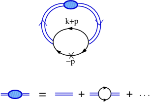
Figure 2: Diagram determining the density at leading order in $z^{2}$ (top) and the dressing of the dimer propagator.

We can understand now the reason for the resummation of graphs at the bottom of Fig. (2). For momenta of order $p\sim\sqrt{MT}\sim 1/a$, the square root in the denominator of Eq. (7), generated by the loops in the dimer propagator, is not negligible compared to $1/a$.

Plugging the expression in Eq. (7) in the diagram in Fig. (2) we have

$$n_{2}^{(2)} = MT\sum_{k_{0}}\int\frac{d^{3}k}{(2\pi)^{3}}\frac{1}{-\frac{1}{a}+\sqrt{\frac{\vec{k}^{2}}{4}-2M\mu-iMk_{0}}}\frac{1}{\sqrt{\frac{\vec{k}^{2}}{4}-2M\mu-iMk_{0}}}$$ (8)

$$= MT\int\frac{d\eta}{2\pi i}\int\frac{d^{3}k}{(2\pi)^{3}}\frac{1}{e^{\beta\eta}-1}\frac{1}{-\frac{1}{a}+\sqrt{\frac{\vec{k}^{2}}{4}-2M\mu-M\eta}}\frac{1}{\sqrt{\frac{\vec{k}^{2}}{4}-2M\mu-M\eta}}\ .$$

The integration over $\eta$, on a contour encircling the imaginary axis, can be deformed into an integral over the discontinuity on the branch cut (which describes the dimer break up) plus the contribution of the dimer pole. The final result is

$$n_{2}^{(2)}=2b_{2}\frac{z^{2}}{\lambdabar^{3}}=\frac{z^{2}}{\lambdabar^{3}}\ \ e^{\beta B_{2}}\ \ 2^{3/2}\left(1+\mathrm{Erf}\left(\frac{1}{a\sqrt{MT}}\right)\right)\ ,$$ (9)

where $B_{2}=1/(Ma^{2})$ is the location of the pole in the dimer propagator. This pole corresponds to a bound state (if $a$ is positive) or a “virtual” bound state, that is, a pole in the unphysical sheet (if $a$ is negative). Eq. (9) is a particular case of the classic formula relating $b_{2}^{(2)}$ to the two-particle scattering phase shift  [18]

$$b_{2}^{(2)}=2^{1/2}\left(e^{\beta B_{2}}+\frac{1}{\pi}\int_{0}^{\infty}dk\frac{d\delta(k)}{dk}e^{-\frac{\beta k^{2}}{M}}\right)\ ,$$ (10)

in the case where the phase shifts are given by the leading order effective range expansion $k\cot\delta(k)=-1/a$. A few points are worth mentioning here. First, $b_{2}$ is a continuous function of $a$ at $1/a=0$. The change in the potential needed to take $a$ from a large and positive value to a large and negative value is small, and that change has only a small effect in the thermodynamics, even though there is a qualitative difference in the spectrum (from a bound state to a virtual bound state). Second, $b_{2}$ is positive and, for $B_{2}>T$, it is exponentially large. In the case $a>0$, this is easily understood as a consequence of the existence of a bound state: when $T\ll B_{2}$ most particles form tight two-body bound states therefore increasing the density for a fixed temperature and chemical potential. In fact, if the $z^{2}$ terms dominate, the ratio of the two equations in Eq. (1) give the equation of state of a free gas with density $n/2$.

The third virial coefficient $b_{3}$ includes three pieces. The first, $b_{3}^{(1)}$, is determined by the $z^{3}$ piece in Eq. (4) and equals $b_{3}^{(1)}=3^{-\frac{5}{2}}$. The second one, $b_{3}^{(2)}$, comes from a subleading piece of the diagram on Fig. (2) and is given by

$$n_{3}^{(2)} = 3\ b_{3}^{(2)}\ \frac{z^{3}}{\lambdabar^{3}}$$

$$= 2\ T\sum_{k_{0}}\int\frac{d^{3}k}{(2\pi)^{3}}\left[({\mathcal{D}}^{(0)}(k))^{2}\Sigma^{(1)}(k)\frac{d}{idk_{0}}\Sigma^{(0)}(k)+{\mathcal{D}}^{(0)}(k)\frac{d}{idk_{0}}\Sigma^{(1)}(k)\right]$$

$$= 2\ T\sum_{k_{0}}\int\frac{d^{3}k}{(2\pi)^{3}}\frac{d}{dk_{0}}({\mathcal{D}}^{(0)}(k)\Sigma^{(1)}(k))$$

$$= \frac{i\beta z^{3}}{\pi^{4}}\int_{0}^{\infty}dk^{2}\int_{0}^{\infty}dp\int d\zeta e^{-\beta\frac{p^{2}}{2M}}{\rm arctgh}(\frac{p\ k}{k^{2}+\frac{p^{2}}{2}-2M\mu-iMp_{0}})\frac{1}{-\frac{1}{a}+\sqrt{\frac{k}{4}-M\zeta}},$$

where the integral over $\zeta$ runs on a vertical line just to the left of the pole at $-B_{2}$. The integral in Eq. (I) cannot be expressed analytically and has to be computed numerically.

Figure 3: Graph determining the density at leading order in $z^{3}$ and the integral equation for the three-body amplitude.

The third piece, $b_{3}^{(3)}$, comes from actual three-body correlations in the system, and brings in new physics besides that contained in two-body scattering. The diagrams contributing to it are shown on Fig. (3). Just as the two-body scattering amplitude cannot be computed in perturbation theory, the three-body amplitude that enters in Fig. (3) also involves a resummation of an infinite number of diagrams. This is because each additional loop involves a factor of $pa$, where $p$ is the typical momentum flowing through the loop. In the case considered here $Q\sim 1/\lambdabar\sim 1/a$ and the “suppression” factor is of order $1$. The diagrams in Fig. (3) gives

$$n_{3}^{(3)} = T^{2}\sum_{k_{0},p_{0}}\int\!\!\frac{d^{3}k}{(2\pi)^{3}}\frac{d^{3}p}{(2\pi)^{3}}\left(\frac{1}{ip_{0}+\epsilon_{p}}\right)^{2}{\mathcal{D}}^{(0)}(p+k){\mathcal{T}}(-p,p+k;-p,p+k)$$

$$= T^{2}\sum_{k_{0}}\int\!\!\frac{d^{3}k}{(2\pi)^{3}}\frac{d^{3}p}{(2\pi)^{3}}\frac{d\eta}{2\pi i}\frac{1}{e^{\beta\eta}-1}\left(\frac{1}{\eta+\epsilon_{p}}\right)^{2}{\mathcal{D}}^{(0)}(p+k){\mathcal{T}}(-p,p+k;-p,p+k)$$

where in the second line $p=(-i\eta,\vec{p})$ and ${\mathcal{T}}(-p,p+k;-p,p+k)$ is the forward particle-dimer scattering amplitude determined by the diagrams at the bottom of Fig. (3). The integral over $\eta$ is dominated by the particle pole at $\eta=-\epsilon_{p}$, with the contribution coming from the dimer pole and cut suppressed by two powers of $z$. We then have

$$n_{3}^{(3)} = -\frac{2\pi z^{3}}{g^{2}}\int\frac{d^{3}k}{(2\pi)^{3}}\frac{d^{3}P}{(2\pi)^{3}}\int\frac{d\zeta}{2\pi i}e^{-\beta\zeta}\ {\mathcal{T}}(-P+\frac{k}{3},P+\frac{2k}{3};-P+\frac{k}{3},P+\frac{2k}{3})|_{k_{0}=i3\mu-i\zeta}$$ (13)

$$\ \ \ \ \ \ \ \ \ \ \frac{1}{-\frac{1}{a}+\sqrt{\frac{3\vec{P}^{2}}{4}+\frac{\vec{k}^{2}}{6}-M\zeta}}\frac{1}{\sqrt{\frac{3\vec{P}^{2}}{4}+\frac{\vec{k}^{2}}{6}-M\zeta}},$$

where we use the center-of-mass variable $P=(i\epsilon_{p},\vec{p}+\vec{k}/3)$. The integration over the new variable $\zeta=3\mu+\zeta$ in on a vertical line just to the left of the left-most singularity that can be a trimer pole at $k^{2}/6M-B_{3}$ or a dimer pole at $k^{2}/6M+3P^{2}/4M-B_{2}$. The cuts in the three-body amplitude describing dimer-particle scattering, dimer breakup, etc., are on the real axis, to the right of $2$ and $3$ particle poles.

Unlike the dimer propagator, the diagrams adding up to the three-body amplitude ${\mathcal{T}}(-p,p+k;-p,p+k)$ do not form a simple geometrical series and cannot be summed up analytically. However, their sum is determined by the integral equation depicted at the bottom of Fig. (3). This integral equation (Faddeev equation) is particularly simple for the separable potential used here and was derived many times before with a variety of techniques  [20, 21, 22]. It is more easily written in terms of the $s-$wave amplitude ${\mathcal{T}}_{0}(\zeta,P,P^{\prime})$ defined by

$$Mg^{2}\frac{{\mathcal{T}}_{0}(\zeta,P,P^{\prime})}{\vec{P}^{2}-\frac{4M}{3}(\zeta+B_{2})}=\int\frac{d\hat{P}}{4\pi}\frac{d\hat{P^{\prime}}}{4\pi}\frac{{\mathcal{T}}(-P+\frac{k}{3},P+\frac{2k}{3};-P+\frac{k}{3},P+\frac{2k}{3})|_{k_{0}=i3\mu-i\zeta}}{-\frac{1}{a}+\sqrt{\frac{3\vec{{P^{\prime}}}^{2}}{4}+\frac{\vec{k}^{2}}{6}-M\zeta}},$$ (14)

Higher partial waves, describing more peripheral particle-dimer collisions, give suppressed contributions. ${\mathcal{T}}_{0}(\zeta,P,P^{\prime})$ satisfies

$${\mathcal{T}}_{0}(\zeta,P,P^{\prime})=K(\zeta,P,P^{\prime})+\frac{2}{\pi}\int_{0}^{\Lambda}dqq^{2}\frac{{\mathcal{T}}_{0}(\zeta,P,q)}{q^{2}-\frac{4M}{3}(\zeta+B_{2})}K(\zeta,q,P^{\prime}),$$ (15)

with the kernel

$$K(\zeta,P,P^{\prime})=\frac{4}{3}\left(\frac{1}{a}+\sqrt{\frac{3P^{2}}{4}-M\zeta}\right)\left[\frac{1}{PP^{\prime}}\log\left(\frac{P^{2}+PP^{\prime}+{P^{\prime}}^{2}-M\zeta}{P^{2}-PP^{\prime}+{P^{\prime}}^{2}-M\zeta}\right)-\frac{g_{3}(\Lambda)}{Mg^{2}}\right]$$ (16)

Eq. (15) has a number of surprising properties  [23, 24, 25, 26, 27]. This properties are more naturally described in terms of renormalization theory. It was shown in  [28, 29] that ${\mathcal{T}}_{0}(\zeta,P,P^{\prime})$ is kept cutoff independent for small values of $P,P^{\prime}\ll\Lambda$ if, and only if, the three-body force varies with the cutoff $\Lambda$ as

$$-\frac{g_{3}(\Lambda)\Lambda^{2}}{2Mg^{2}}=\frac{\sin(s_{0}\log(\Lambda/\Lambda^{*})-\arctan s_{0})}{\sin(s_{0}\log(\Lambda/\Lambda^{*})+\arctan s_{0})}+{\mathcal{O}}(\frac{1}{a\Lambda}),$$ (17)

where $\Lambda^{*}$ is a new parameter that cannot be measured through two-particle experiments and $s_{0}\approx 1.006$ is the solution of a certain trigonometric equation. The failure to include the three-body force term leads to a strong cutoff dependence on the results and thus, to the impossibility of arriving at model independent results. The three-body scattering amplitude depends, even at the leading order in the expansion in powers of $\lambdabar/R$, on the value of the three-body force, here parameterized by $\Lambda^{*}$. The parameter $\Lambda^{*}$ encodes all short distance physics, besides the value of $a$, necessary to describe three-body systems. Like $a$, it varies from one system to another and only the measurement of some three-body observable allows us to fix it. The appearance of an extra parameter not determined by two-body scattering precludes the possibility of predictions in the three-body sector based only on the value of $a$.

Using Eq. (13) and Eq. (14) and performing a trivial integral over $k$ and the angular part of $\vec{P}$ we arrive at

$$n_{3}^{(3)}=3b_{3}^{(3)}\frac{z^{3}}{\lambdabar^{3}}=i\frac{9\sqrt{3}}{4\pi^{2}}M\frac{z^{3}}{\lambdabar^{3}}\int_{0}^{\infty}\!\!dPP^{2}\!\!\int\!\!d\zeta e^{\beta\zeta}\frac{{\mathcal{T}}_{0}(\zeta,P,P)}{(\frac{3P^{2}}{4}-M\zeta-B_{2})^{2}}\left(1+\frac{1}{a}\frac{1}{\sqrt{\frac{3P^{2}}{4}-M\zeta}}\right)$$

The amplitude ${\mathcal{T}}_{0}(\zeta,P,P)$ and the quadratures in Eq. (I) have to be performed numerically. This is not computationally demanding and a Mathematica notebook that performs this task can be downloaded from http://www-nsdth.lbl.gov/b̃edaque.

The coefficient $b_{3}=b_{3}^{(1)}+b_{3}^{(2)}+b_{3}^{(3)}$ is a function of the temperature and of the parameters describing the microscopic dynamics (the scattering length $a$ and the three-body parameter $\Lambda^{*}$). In Fig. (4) we show the value of $b_{3}$ as a function of $1/a$ for a few values of these parameters. As an example we pick $M=M_{{}^{4}{\rm He}}$, $T=10^{-7}{\rm eV}\approx 1.16mK$ and $-\Lambda^{2}g_{3}(\Lambda)/(2Mg^{2})\equiv H(\Lambda)=-3.235$ (lower blue solid curve), $-0.22$ (intermediate red solid curve) and $0.05$ (upper black solid curve). In all of them we use $\Lambda=200$ eV, but, as mentioned above, the results are cutoff independent up to small corrections of order $1/\Lambda a$. The first of these values was chosen following  [30] and it gives rise to a trimer with the binding energy of the shallower ⁴He trimer (as predicted through potential model calculations  [31, 32, 33] ) when $a$ is set to the value inferred from the dimer measurement $a=10^{+8}_{-18}\mathring{A}$  [34]. For the value of the $\Lambda$ used the deeper trimer state is absent.

When $a$ and $\Lambda^{*}$ are such that there is a three-body bound state $B_{3}\gtrsim B_{2}$, we find empirically that $b_{3}$ scales roughly as $e^{\beta B_{3}}$, see Fig. 4. This is not surprising and is a direct analogue of the physics described by Eq. (9) in the case of the coefficient $b_{2}$: when $\beta B_{3}\gg 1$ most particles form three-body bound states, which increases the density for a given temperature and chemical potential as compared to the free gas. This does not mean, however, that the integral in Eq. (I) is dominated by the trimer pole: the contribution from the two-and three-particle cuts is never negligible. For values of $a\Lambda^{*}$ for which $B_{3}$ approaches $B_{2}$ the dimer-particle cross section diverges. Still, the three-particle correlations described by $b_{3}$ are smooth at those points. For systems with a trimer deeper than the dimer, $b_{3}$ can be much larger that both $b_{1}$ and $b_{2}$, and dominate the virial expansion. This is not a rare situation, due to a well known but strange feature of the three-resonating particle system: as the potential is changed to make the dimer shallower , the trimer becomes deeper  [25]. This is what happens in the $H=0.05$ case shown in the upper (black) solid curve in Fig. 4.

In atomic traps close to a Feshbach resonance it is $a$ that is a tunable parameter. The influence of the magnetic field on the value of the three-body force parameter $\Lambda^{*}$ is small, since that describes short-distance physics of an energy scale much higher than the magnetic field, and can be disregarded in a first approximation. Thus we can regard the horizontal axis in Fig. (4) as denoting the magnetic field using the Feshbach resonance formula

$$a(B)=a(B=0)\left(1+\frac{\delta B}{B-B_{0}}\right).$$ (18)

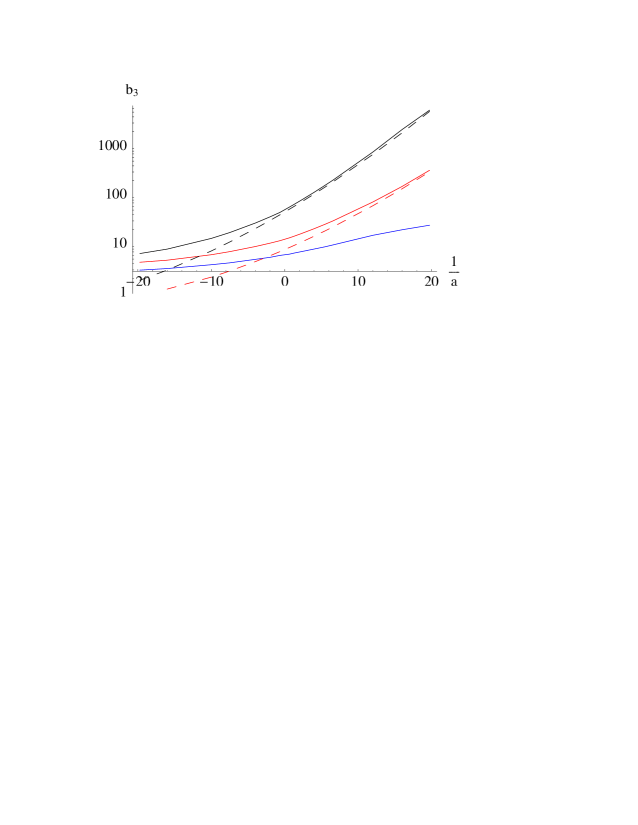
Figure 4: $b_{3}$ as a function of the inverse scattering length for three values of $H(\Lambda=200{\rm eV})$ (solid lines, $H=-3.23,-0.22,0.05$, from bottom to top). The dashed line is the estimate $e^{\beta B_{3}}$.

Let us summarize the approximation performed here that allowed such a simple evaluation of such a complex three-body dynamics. First, we approximate the two-body potential by a short range, delta-function-like interaction. Corrections to this approximation are proportional to the effective range $r_{0}/\lambdabar$, where $r_{0}\sim R$ is the effective range, much smaller than $a$ by assumption. Effective range corrections can be easily included, even to very high orders, without spoiling the simplicity of the method, as it has been done in few-nucleon physics  [22, 35]. The second approximation was the non-inclusion of higher partial waves. In the two-body sector, $p$-waves and higher are suppressed by at lest two powers of $R/\lambdabar$, and are small. In the three-body sector the suppression of the particle-dimer $l$-wave interactions are not suppressed by powers of $R/\lambdabar$, but by $1/(l+1)$. All the higher partial waves correspond to a repulsive kernel in Eq. (15), which do not support bound states and cannot produce an enhancement of the form $e^{\beta B_{3}}$. In practice the phase shifts are rather small but, if needed, they can also be easily included by solving the analogue of Eq. (15) corresponding to the higher partial wave and adding it to Eq. (13).

Our results are valid only in true thermal equilibrium, after two- and three-particle bound states had the time to form, and assuming that they stay in the system ( do not escape from the trap, if that is the case). For systems like the alkali atoms studied in magnetic/optical traps, that have deep bound states with typical interparticle distance of order $\sim R$ that lie outside the validity range of our effective theory, this means that our results are relevant only for the metastable state before the collapse of the system, but after the two- and three-body bound states form. The formation of a $l-$body bound state requires the approach of $l+1$ particles in order to conserve energy and momentum, and their rates are consequently suppressed by $n^{l+1}$. These rates are not known at finite temperature but have been studied at zero temperature in  [36, 37, 38] (recombination into shallow states) and  [39] (recombination into deep states). In cases where $a>0$ the recombination rate into deep (two-body) bound states is estimated to be much smaller than the rate into shallow bound states suggesting that there is a time window in which our results apply. In the $a<0$ case there is no two-body bound state and it is not known how the rates for the formation of deep and shallow three-body bound states compare.

Finally, let us consider the changes introduced in case of fermionic particles. In the non-degenerate case considered here, the effect of the quantum statistics in the thermodynamics is minor, and amounts to a change in sign in some of the coefficients $b_{1,2}^{(1,3,...)}$. The elementary collisions, however, may differ a great deal due to the exclusion principle. If we have only one fermionic species in the system, $s$-wave scattering is impossible and all virial coefficients $b_{2},b_{3},\cdots$ are suppressed. In the case of two fermionic species (as a dilute neutron gas), two-body collisions are possible and the standard result in Eq. (9) is valid. The physics of the three-body correlations is however, very different. No three-body force term without derivatives exist, and the three-body force contribution is suppressed. $b_{3}$ can be computed in terms of $a$ alone, but cannot ever be large and dominate the expansion, as the kernel appearing in Eq. (15) would be repulsive and would not support a bound state. The case with three or more fermionic species with all the scattering lengths large but not necessarily equal, which includes the dilute nuclear matter case (protons and neutrons with spin either up or down), is very similar to the bosonic case. Three particles can occupy the same point in space without violating the exclusion principle and, as a consequence, the two coupled equations that substitute Eq. (15) have very similar properties to the bosonic equation  [40].