An extremal model for amorphous media plasticity

Abstract

An extremal model for the plasticity of amorphous materials is studied in a simple two-dimensional anti-plane geometry. The steady-state is analyzed through numerical simulations. Long-range spatial and temporal correlation in local slip events are shown to develop leading to non-trivial and highly anisotropic scaling laws. In particular, the plastic strain is shown to statistically concentrate over a region which tends to align perpendicular to the displacement gradient. By construction, the model can be seen as giving rise to a depinning transition, the threshold of which (i.e. the macroscopic yield stress) also reveal scaling properties reflecting the localization of the activity.

In contrast with crystalline solids, amorphous materials display a plasticity which cannot be resumed to the motion of well identified defects such as dislocations. Consequently, the microscopic description of amorphous plasticity is still lacking a consistent framework. Recent studies [1, 2, 3, 4] have focussed on the fact that global plastic deformation is mostly due to local rearrangements. Starting from a molecular dynamics study of a bidimensional Lennard-Jones glass and measurements of the mechanical response under shear stress, Falk and Langer[4] introduced the notion “Shear Transformation Zones” (STZ) having a bistable character to build a mean field theory of plastic deformation in an amorphous material. Initially drawn by Bulatov and Argon [1, 2, 3] for amorphous solids materials this approach can be extended to granular materials or dense suspensions[5, 6]. In the following we study a minimal model of plastic deformations in disordered media. This model has been proposed in the early eighties to describe the fault self-organization in seismic regions[7, 8] where mostly the “avalanche” properties of this model were studied in order to compare with the observed power-law distribution of seismic events (Gutenberg-Richter law). In [8], a quenched random distribution of local threshold stress was introduced which allowed for a mapping onto a random polymer problem in the limit of vanishing stress drop. The analysis we propose focuses on the scaling feature of the spatio-temporal organization of the local slip events and on the stress-strain characterization.

We consider a bidimensional material submitted to anti plane shear stress. The elastic component of the displacement $u_{z}(x,y)$ is thus solution of a Laplace equation $\nabla^{2}u_{z}=0$. The material is discretized on a regular lattice, the axis of which are oriented at 45 degrees from the displacement gradient direction. The elastic modulus is assumed to be uniform but we impose a spatially frozen disorder for the onset of slip at a local level. After a local slip, we renew the threshold stress where the slip occured from a random distribution. Bi-periodic boundary conditions are implemented for the stress and the strain, whereas a discontinuity is imposed on the displacement along the $y$ axis. We choose an extremal dynamics: the external load $\Sigma$ is adjusted at each step so that only one bond is at the plastication threshold. In the spirit of Ref.[4], this corresponds to a structural rearrangement of a “shear transformation zone”. The latter induces a displacement discontinuity along the bond and a random modification of the plastication threshold. The local stress is redistributed over the material according to the elastic response function. The local stress on a bond $i$ is $\sigma_{i}=\Sigma+\sigma_{i}^{o}$ where $\Sigma$ is the macroscopic stress. After a slip $\Delta u_{j}$ at bond $j$, $\sigma_{i}^{o}$ is adjusted to $\sigma_{i}^{o}=\sigma_{i}^{o}+\Delta u_{j}G(\underline{x_{i}}-\underline{x_{j}})$. Apart from the periodicity imposed by the boundary conditions, this function $G(\underline{x})$ is long ranged, decreasing as $G(\underline{x})\propto|\underline{x}|^{-2}$. Moreover, due to the shear boundary condition, the stress redistribution is anisotropic. In the longitudinal $x$ direction, bonds are loaded while in the transverse $y$ direction they are unloaded. This anisotropy is one distinct feature of the model leading to the localization effect to be described below.

The local plastication thresholds $\gamma(x,y)$ are randomly chosen according to a uniform distribution between 0 and 1. Since the elastic modulus is uniform, the stress redistribution is computed once and for all via a conjugated gradient algorithm, for a local slip of unit magnitude. This effective Green function is then simply translated to the location of the slip event and its amplitude is scaled by the slip magnitude (also assumed to be random).

The behavior of this model is of the pinning/depinning type. The plastication criterion of an individual bond can be written $\Sigma^{ext}>\gamma(x,y)-\sigma^{el}(x,y)$ where $\sigma^{ext}$ is the external shear stress, $\gamma(x,y)$ the local plastication threshold and $\sigma^{el}(x,y)$ the local stress component due to elastic stress redistribution from previous plastication events. Following an extremal dynamics, we select at time $t$ the current “weakest site” $(x^{*},y^{*})$ such that $\sigma_{c}(t)=\gamma(x^{*},y^{*})-\sigma^{el}(x^{*},y^{*})=\min_{(x,y)}[\gamma(x,y)-\sigma^{el}(x,y)]$. The maximum over time $\sigma^{*}=\max_{t}\sigma_{c}(t)$ corresponds to the macroscopic yield stress. From this signal we can reconstruct the evolution of the system subjected to a constant load: when submitted to an external shear stress lower than $\sigma^{*}$ the plate deforms plastically before blocking in a jammed state. For values above the yield stress, the system flows indefinitely.

Such pinning systems have been extensively studied over the recent years. They have been used to describe front motion in a disordered environment in the context of wetting[9], magnetic domain walls [10], fluid invasion in porous media [11], crack propagation [12, 13, 14]; or the behavior of ‘periodic systems’, e.g. vortex lattices [15] or charge density waves (CDW) [16].

Beyond the yielding transition, this simple model exhibits another characteristic feature of plasticity: hardening (i.e. increase of the yield stress with the plastic strain). In crystalline solids, the hardening behavior is due to the entanglement of dislocation loops. In the present case, after a first loading, we observe an increase of the elastic limit. However the mechanism for this hardening effect is here of a pure statistical nature. During the loading process, the weakest sites are progressively decimated. Then the plastic threshold $\gamma(x,y)$ is renewed. The new threshold is in average larger than the previous one. This introduces a systematical bias. When submitted for the first time to a loading process, the distribution of these local plastication thresholds evolves to eventually reach a stationary state. On Fig. 1, we show the evolution of the mean plastication threshold $\langle\gamma(x,y)\rangle$ during loading. The asymptotic steady distribution seems not reached yet on the figure. This hardening effect thus corresponds to a progressive reinforcement of the weakest regions.

On Fig. 2 (above) we show a map of the cumulative plastic strain for a system of size $128\times 64$ after $810^{5}$ time steps. We see clearly that the plastic strain is non uniform: it is localized within regions elongated along the $x$ direction. Focusing on the plastic deformation taking place within a finite time window, we show on the same figure (below) the appearance of an individual localized structure. To characterize quantitatively this spatial distribution, we studied the pair correlation function of the plastic strain $\varepsilon_{p}(x,y)$ through Fourier transforms of the strain map averaged over time. We found that the projection of the plastic strain along the $x$ or $y$ axis, $\varepsilon_{\parallel}(x)=\langle\varepsilon_{p}(x,y)\rangle_{y}$ and $\varepsilon_{\perp}(y)=\langle\varepsilon_{p}(x,y)\rangle_{x}$ are self-affine profiles with roughness exponents $\zeta_{\parallel}\approx-0.09$ and $\zeta_{\perp}\approx 0.50$. Figure 3 shows the power spectra of $\varepsilon_{p}$ for $k_{x}=0$ and $k_{y}=0$, where the power-law behaviors give directly the cited roughness exponents.

Such a scaling behavior which characterizes the steady state fluctuations of the cumulative strain allows to analyze the time evolution of the plastic flow. Let us consider two local slip events separated by a time lapse $\tau$, and record their distance along the $x$ and $y$ direction, noted respectively $d_{\parallel}$ and $d_{\perp}$. Averaging over time (at fixed $\tau$), the probability distribution function of these distances $p(d,\tau)$ reveal two characteristic “correlation lengths”, $\xi_{\parallel}$ and $\xi_{\perp}$, below which $p$ is constant, and above which $p$ decays as a power-law with an exponent $\alpha_{\parallel}$ or $\alpha_{\perp}$ respectively. Varying the time lapse $\tau$, we observe that

$$\xi_{\parallel}(\tau)\propto\tau^{1/z_{\parallel}}\qquad\xi_{\perp}(\tau)\propto\tau^{1/z_{\perp}}$$ (1)

Exploiting the self-affine nature of the cumulative plastic strain, and using a result obtained for other extremal models of depinning, we can relate the two dynamic exponents to the roughness exponents:

$$z_{\parallel}=1+\zeta_{\parallel}\qquad z_{\perp}=1+\zeta_{\perp}$$ (2)

The numerical values of the $z$ exponents are consistent with these identities.

The difference in scaling in the $x$ and $y$ direction can be accounted for through a power-law relating both directions. Indeed, the correlation lengths are related through $\xi_{\perp}\propto\xi_{\parallel}^{\beta}$ with $\beta=z_{\parallel}/z_{\perp}\approx 0.65$. Moreover, looking at the mean value of $d_{\perp}$ for a prescribed value of $d_{\parallel}$ also reveal the same power-law $d_{\perp}\propto d_{\parallel}^{\beta}$, with $\beta\approx 0.65$.

Let us focus now on the depinning stress distribution. On Fig. 4 we show the distribution of the local plastication stresses, $\gamma(x,y)-\sigma^{el}(x,y)$ (at all sites and all times) and of the current plastication stresses, $\sigma_{c}(t)$. The maximum of the latter over time corresponds to the macroscopic yield stress $\sigma^{*}$. We clearly see that the yield stress separates two distinct regions. Stresses larger than $\sigma^{*}$ are approximately distributed according to a normal law. Stresses lower than $\sigma^{*}$ are however distributed according to a power law of the argument $(\sigma^{*}-\sigma)$. As above suggested the fraction of sites such that $\sigma<\sigma^{*}$ can be thought of as a population of potential active sites and hence may be interpreted as potential STZ. Let us emphasize that these STZ are not postulated but emerge naturally within the model.

Prior to a large jump in the location of the slip event, the lattice has reached a state of strong pinning. Hence, following the analysis presented in Ref. [17], if we condition the statistical distribution of $\sigma_{c}(t)$ by the distance to the location of the next slip event, along the $x$ direction for instance, $\Delta x$, we observe that the larger $\Delta x$, the narrower the distribution and the closer its mean to the yield stress $\sigma^{*}$. These distributions are shown in Fig. 5. Motivated by the underlying criticality of the depinning transition, we may anticipate a scaling form of the distribution as

$$p(\sigma_{c}|\Delta x)=\Delta x^{\nu_{\parallel}}\psi\left[(\sigma^{*}-\sigma_{c})\Delta x^{\nu_{\parallel}}\right]\;.$$ (3)

This particular form implies that the standard deviation of the distribution, $\delta\sigma_{c}$ vanishes as $(\Delta x)^{-\nu_{\parallel}}$, and that the mean value of $\langle\sigma^{*}-\sigma_{c}\rangle(\Delta x)$ is simply proportional to $\delta\sigma_{c}(\Delta x)$. The first property allows to determine $\nu_{\parallel}$ and the second gives a simple way to estimate precisely $\sigma^{*}$ through a simple linear regression. The same procedure applied to $\Delta x$ gives a similar result. Using the linear dependence of $\delta\sigma_{c}$ on $\sigma_{c}$ conditioned to the size of the activity jump in both the $x$ and $y$ direction, we find numerically $\sigma^{*}=0.517$ for a uniform distribution of threshold $\gamma$ in $[0,1]$ and a random slip amplitude from the same distribution.

The scaling of the standard deviation of the distribution versus the jump size gives a determination of the exponents $\nu_{\parallel}\approx 0.68$ and $\nu_{\perp}\approx 0.98$. We note that again the ratio of these exponents gives the anisotropy scaling $\beta=\nu_{\parallel}/\nu_{\perp}=0.69$ in good agreement with the previous determinations ($\beta\approx 0.65$).

The knowledge of the distribution $p(d)\propto d^{-\alpha_{\parallel}}$ of the $x$-distances between successive active sites allows to express the depinning stress distribution close to threshold:

$${\cal Q}(\sigma^{*}-\sigma_{c}) = \int x^{\nu_{\parallel}-\alpha_{\parallel}}\psi\left[(\sigma^{*}-\sigma_{c})x^{\nu_{\parallel}}\right]dx$$ (4)

$$\propto (\sigma^{*}-\sigma_{c})^{\mu}\;$$ (5)

where

$$\mu={\frac{\alpha_{\parallel}-\nu_{\parallel}-1}{\nu_{\parallel}}}$$ (6)

The same argument obviously also holds for the $y$ direction. This latter scaling is also consistent with the anisotropy scaling $\beta=(\alpha_{\parallel}-1)/(\alpha_{\perp}-1)\approx 0.64$.

Despite its extreme simplicity, the model that we presented accounts for several features of plasticity in amorphous materials. We could identify a macroscopic yield stress. Below this threshold, the material deforms plastically before blocking in jammed state. Above, it can flow indefinitely. This behavior is typical of a pinning/depinning situation. In the same spirit as the study presented in Ref.[17], the model exhibits a critical behavior of the plastic stress close to the macroscopic yield stress. When submitted for the first time to a shear stress we observe a hardening effect. In contrast with crystalline materials, here this effect is of a pure statistical nature and corresponds to a progressive reinforcement of the weakest regions. In addition to this global hardening plastic behavior, the model exhibits a statistical localization. The latter appears via elongated structures in the shear direction. However, instead of concentrating onto a unique structure (such as in Ref. [8]), the plastic strain develops a complex spatio-temporal organization. A statistical analysis of these patterns reveals scaling properties; scaling exponents are summarized in table I.

Beyond this simplified model, the introduction of thermal activation in the selection of the site to plastify should allow to account for visco-plastic effects. Another improvement of such models would consist in including both deviatoric and volumetric strain, the latter coupling being characteristic of irreversible deformation in amorphous solids.

$\zeta_{\parallel}$	=	$-0.09\pm 0.05$	$\zeta_{\perp}$	=	$0.50\pm 0.05$
$\alpha_{\parallel}$	=	$1.61\pm 0.05$	$\alpha_{\perp}$	=	$1.96\pm 0.05$
$\nu_{\parallel}$	=	$0.68\pm 0.05$	$\nu_{\perp}$	=	$0.98\pm 0.05$
$\mu$	=	$0.00\pm 0.05$	$\beta$	=	$0.65\pm 0.05$

TABLE I.: Table of scaling exponents

FIG. 1.: Evolution of the mean plastication threshold $\langle\gamma(x,y)\rangle$ during the transient regime of a first loading process. The increase of $\langle\gamma(x,y)\rangle$ can be interpreted as a hardening effect.

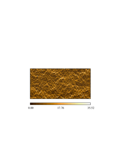
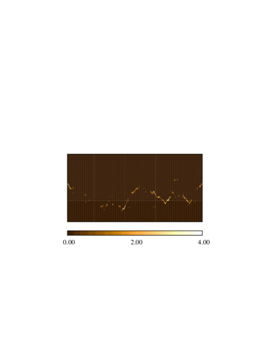
FIG. 2.: Map of the relative displacement field obtained on a system $128\times 64$ after 800 000 times steps (above). The diffuse localization corresponds to the succesive development of anisotropic structures elongated in the longitidinal direction. Focusing on a finite time window (450 time steps, below) allows to reveal an individual structure.

FIG. 3.: Power spectra of the plastic strain $\varepsilon_{p}$ for $k_{x}=0$ (circles) and $k_{y}=0$ (squares). The lines indicate power law behaviors corresponding to roughness exponents $\zeta_{\parallel}=-0.09$ and $\zeta_{\perp}=0.50$

FIG. 4.: Distribution of the individual site plastication thresholds $\sigma_{i}$ (line) (all sites, all times) and of the current plate plastication thresholds $\sigma_{c}$ (dotted line) (active site, all times). The vertical line indicates the position of the yield stress $\sigma^{*}$.

FIG. 5.: Distribution of depinning stress (bold) and contributions conditionned by the distances (2,4,8,16,32) between consecutive active sites. The tail of the distribution corresponds to very short jumps and is very sensitive to the details of the random threshold distribution. The contributions obtained for increasing distances between consecutive active sites present the same trend: the larger the jump, the closer the mean force to the threshold and the narrower the distribution. After rescaling (inset) these distributions collapse onto a single master curve.

REFERENCES

- [1] V.V. Bulatov and A.S. Argon, Modell. Simul. Mater. Sci. Eng. 2 167, (1994).
- [2] V.V. Bulatov and A.S. Argon, Modell. Simul. Mater. Sci. Eng. 2 185, (1994)
- [3] V.V. Bulatov and A.S. Argon, Modell. Simul. Mater. Sci. Eng. 2 203 (1994).
- [4] M.L. Falk and J.S. Langer, Phys. Rev. E 57, 7192 (1998).
- [5] A. Lemaître, arXiv:cond-mat/0107422
- [6] A. Lemaître, arXiv:cond-mat/0108442
- [7] K. Chen, P. Bak and S.P. Obhukhov, Phys. Rev. A 43, 625 (1991).
- [8] P. Miltenberger, D. Sornette and C. Vanneste, Phys. Rev. Lett. 71, 3604 (1993).
- [9] E. Rolley, C Guthmann, R. Gombrowicz and V. Repain, Phys. Rev. Lett. 80, 2865 (1998).
- [10] S. Lemerle, J. Ferré, C. Chappert, V. Mathet, T. Giamarchi, and P. Le Doussal, Phys. Rev. Lett. 80, 849 (1998).
- [11] D. Wilkinson and J.F. Willemsen, J. Phys. A 16, 3365 (1983).
- [12] J. Schmittbuhl, S. Roux, and Y. Berthaud, Europhys. Mett. 28 (8), 585 (1994).
- [13] A. Tanguy, M. Gounelle and S. Roux, Phys. Rev. E 58, 1577 (1998).
- [14] S. Ramanathan and D.S. Fisher, Phys. Rev. B 58, 6026 (1998).
- [15] G. Blatter, M.V. Feigel’man, V.B. Geshkenbein, A.I. Larkin and V.M. Vinokur, Rev. Mod. Phys. 66, 1125 (1994).
- [16] G. Grüner, Rev. Mod. Phys. 60, 1129 (1988).
- [17] R. Skoe, D. Vandembroucq and S. Roux, “Front propagation in random media: from extremal to activated dynamics”, accepted in Int. J. Mod. Phys. C, cond-mat/0203158.