Quasi-classical descendants of disordered vertex models with boundaries

Abstract

We study descendants of inhomogeneous vertex models with boundary reflections when the spin-spin scattering is assumed to be quasi–classical. This corresponds to consider certain power expansion of the boundary-Yang-Baxter equation (or reflection equation). As final product, integrable $su(2)$-spin chains interacting with a long range with $XXZ$ anisotropy are obtained. The spin-spin couplings are non uniform, and a non uniform tunable external magnetic field is applied; the latter can be obtained when the boundary conditions are assumed to be quasi-classical as well. The exact spectrum is achieved by algebraic Bethe ansatz. Having realized the $su(2)$ operators in terms of fermions, the class of models we found turns out to describe confined fermions with pairing force interactions. The class of models presented in this paper is a one-parameter extension of certain Hamiltonians constructed previously. Extensions to $su(n)$-spin open chains are discussed.

PACS N. 02.30.Ik, 75.10.Jm

1 Introduction

Integrable vertex models (VM) in two dimensional classical statistical mechanics are the common seed of many relevant exactly-solved quantum models in one dimension [1, 2]. Famous examples are the $XXX$, $XXZ$, and $XYZ$ Heisenberg chains that find more and more applications in contemporary physics. The key toward this powerful synthesis is to notice that the “scattering” of the degrees of freedom of both the VM and the spin chains is described by the same matrix. The Quantum Inverse Scattering Method (QISM) exploits this fact systematically [3]. The method relies on the observation that transfer matrices $\hat{t}=Tr(T)$ span a one-parameter family of commuting operators if a (scattering) matrix $R$ exists such that $T$, $R$ satisfy the celebrated Quantum Yang-Baxter equation. The equivalence between VM and Heisenberg chains consists in the fact that these models have the same $R$–matrix. Due to the property of the scattering $R(u,v)=R(u-v)\;,\quad\forall u,v\in{\rm\kern 2.40005pt\vrule width=0.39993pt,height=6.28612pt,depth=-0.3014pt\kern-3.00003ptC}$ the integrability of VM is preserved if disorder is added at each lattice site such that the scattering “wave momenta” $u$, $v$ result to be shifted arbitrarily. In this case, however, it is difficult to extract a Hamiltonian. A route to simplify the problem is to resort the so called “quasi-classical” limit of the QISM. The term “quasi-classical” here indicates that the scattering between the degrees of freedom of the model is assumed to be quasi-classical. Quantitatively, this means that a parameter $\eta$ does exist such that the scattering matrix is of the form $R(u)\propto{\rm 1\kern-2.20001ptl}\otimes{\rm 1\kern-2.20001ptl}+\eta r(u)$ in the limit $\eta\rightarrow 0$ ($\eta$ plays the role of $\hbar$). The quantity $r(u)$ fulfills the classical Yang-Baxter equation (that is a restatement of the Jacobi identity for the Poisson brackets of suitable action-angle variables). It is worthwhile to mention, however, that the systems obtained by this quasi-classical expansion consist of quantum spins (by no means quasi-classical). The quasi-classical expansion of the transfer matrix of disordered VM (in the lowest spin representation) is non trivial and it produces the Gaudin’s magnet Hamiltonians[4, 5] containing a long range spin interaction (in contrast with the range of the Heisenberg chains which involves nearest neighbour spins).
A richer variety of integrable models by QISM comes from imposing non trivial boundary conditions different from the periodic ones. Twisted boundary conditions, for example, imposed to the six vertex model [6] produce the Gaudin magnet in a non-uniform local magnetic field, which is very important for physical applications. In fact having realized the (pseudo)spin algebra in terms of fermions the $XXX$ Gaudin Hamiltonians in a non uniform magnetic field are the constants of the motion of the BCS model[7] that describes pairs of electrons (in time reversed states) interacting with a long range uniform pairing coupling. The exact solution of the BCS model was found long ago by Richardson[8] and rediscovered recently. In particular it was used to study small metallic grains [9, 10]; the picture was merged in the scenario of QISM in the Ref. [11]. Connections with WZNW models in field theory have been deeply investigated [12] based on the relation between solution of KZ equation and Gaudin model found in Refs. [13, 14]. The class of pairing Hamiltonians was generalized by investigating the quasi-classical expansion of the disordered twisted six vertex model with $XXZ$ $R$-matrix. In terms of fermions this class of Hamiltonians represents interacting electron pairs with certain non-uniform long-range coupling strengths [15, 16, 17, 18]. Twisted rings can be cut to open chains and loops include two reflections at the boundaries. The possibility to include such reflections in integrable theory was founded and systematically investigated by Sklyanin [19]. The quasi-classical limit of the disordered six vertex model with boundaries was investigated first by one of the authors [20, 21]. This led to a model where the spin couplings contain an additional parameter with respect to the original Gaudin magnet, and in a vanishing external magnetic field (see Eq. (27) and the relative discussion below of it). In the present work, we proceed along this line. We still consider an inhomogeneous six-vertex model with boundary reflection, following closely Ref. [20]. By properly choosing the reflection parameters, we introduce an external non-uniform magnetic field of tunable strength in the Hamiltonian. The trick consists in the assumption that also the boundary conditions have a quasi-classical expansion (see Eq. (25) and Sec. 3.2). At best of our knowledge, this idea is pursued for the first time in the present paper. In the following we summarize the main results obtained in the bulk of the paper. The class of spin-$S_{j}$ ($j=1,\dotsc,N$) models that we find has Hamiltonian of the form

$$H=\sum_{j}2h_{j}\hat{S}_{j}^{z}-\sum_{\genfrac{}{}{0.0pt}{}{j,k}{j\neq k}}\left[J_{jk}^{(z)}\hat{S}_{j}^{z}\hat{S}_{k}^{z}+\left(J_{jk}\hat{S}_{j}^{+}\hat{S}_{k}^{-}+h.c.\right)\right]\;.$$ (1)

We agree that the latin indices $j,k$ will run from 1 to $N$, where $N$ is the number of spins. The operators $S^{\pm}\,,\;S^{z}$ are $su(2)$ operators. The couplings are

$$J_{jk}^{(z)} =I_{jk}~{}{\bigl{(}\cosh(2pz_{j})+\cosh(2pz_{k})-2\cos{(2pt)}\bigr{)}}$$

$$J_{jk} =I_{jk}~{}\bigl{(}{\sinh[p(z_{j}-it)]\sinh[p(z_{k}+it)]}\bigr{)}$$

$$I_{jk} =J(\hat{S}^{z})\frac{h_{j}-h_{k}}{\cosh(2pz_{j})-\cosh(2pz_{k})}\;,$$

$$J(\hat{S}^{z}) =J\left(1-J\hat{S}^{z}\right)^{-1}$$ (2)

where $\hat{S}^{z}$ is the total $z$-component of the spin. The quantities $h_{j},z_{j}$ are two arbitrary sets of real parameters; $t$ is also a real arbitrary parameter and it directly comes from the boundary terms (see Eq. (16) with $\xi=it$); finally, $p$ can be $1,i$ or can be tending to zero corresponding to hyperbolic, trigonometric, and rational couplings, respectively.
The eigenstates in the sector with total $z$-component of the spin $S^{z}=\sum_{j}S_{j}-M$, are

$$\left|\Psi\right\rangle=\prod_{\alpha=1}^{M}\hat{S}^{-}(e_{\alpha})\left|H\right\rangle\;,$$ (3)

where

$$\hat{S}^{-}(u)=\sum_{j}\frac{\cosh[p(u+z_{j}+2it)]-\cosh[p(u-z_{j})]}{\cosh(2pu)-\cosh(2pz_{j})}\hat{S}^{-}_{j}$$ (4)

and

$$\left|H\right\rangle=\bigotimes_{j=1}^{N}\left|S_{j}^{z}=S_{j}\right\rangle\;.$$

The corresponding eigenvalues are

$${\mathcal{E}}=\sum_{j}2h_{j}\tau_{i}$$ (5)

where

$$\tau_{j}=S_{j}\left(1-J(S^{z})\sum_{k\neq j}S_{k}\frac{1-x_{j}x_{k}}{x_{j}-x_{k}}+J(S^{z})\sum_{\alpha}\frac{1-x_{j}\lambda_{\alpha}}{x_{j}-\lambda_{\alpha}}\right)\;,$$ (6)

where we defined

$$\frac{1+x_{j}}{1-x_{j}}=\cosh(2pz_{j})-\cos(2pt)\;\;,\;\;\frac{1+\lambda_{\alpha}}{1-\lambda_{\alpha}}=\cosh(2pe_{\alpha})-\cos(2pt)$$ (7)

The rapidities $\lambda_{\alpha}$ satisfy, in the sector having total $z$-component of the spin $S^{z}$, the Bethe equations:

$$\begin{split}&\sum_{\beta\neq\alpha}\frac{1}{\lambda_{\alpha}-\lambda_{\beta}}-\sum_{j}\frac{S_{j}}{\lambda_{\alpha}-x_{j}}+\\ &+\frac{1}{2J(S^{z})}\left(\frac{1+J(S^{z})(1+S^{z})}{1+\lambda_{\alpha}}+\frac{1-J(S^{z})(1+S^{z})}{1-\lambda_{\alpha}}\right)=0\;.\end{split}$$ (8)

We point out that the dependence on the reflection parameters comes only in the couplings and eigenvectors (Eqs. (1)(3)), while the eigenvalues depend on $t$ only implicitely (through Eq.(7)).
The rational limit of the models is recovered for $p\to 0$.
For $t=0$ and $pt=\pi/2$, the models reduce to the ones that we presented in Ref. [15] (see section 3.3). Thus the class of models we discuss in the present paper is a one-parameter extension of the former class.

Using the fermionic realizations of $su(2)$ the Hamiltonian (1) can be rephrased to describe confined fermions interacting with pairing and exchange forces (see Eq. (48)).

The paper is organized as follows. In the next section we summarize the main ingredients of the inverse scattering of VM with boundaries. In section III we construct the integrable models we deal with together with their exact solution. In section IV we use the fermionic realization of the $su(2)$ algebra to rewrite the Hamiltonians in a second quantized form. Section V is devoted to final remarks. In appendix A we review basic properties of VM. In appendix B we prove the integrability of a class of models when a more general (off-diagonal) reflection at the boundary is applied (see Eqs. (51) – (54)). We also discuss a generalization to $su(n)$ case in appendix C.

2 Integrable boundary conditions

In this section, we review how the QISM is applied to VM, in order to obtain a family of commuting transfer matrices. VM describe a system of interacting classical objects on a two dimensional lattice. As described in appendix A, the partition function of the system can be written as $Z=\text{Tr}\{\hat{t}(1)\dotsm\hat{t}(K)\}$, where $\hat{t}(i)$ are operators in some appropriate many-body linear space (in the sense that it is the direct product of $N$ elementary linear spaces). The VM is exactly solvable if $\left[\hat{t}(i),\hat{t}(i^{\prime})\right]=0$. Usually, it is assumed that the dependence on the $i$-th row of the lattice comes through a parameter $u_{i}$, which takes values on some domain of the complex plane. Then the requirement for exact solvability becomes $\left[\hat{t}(u),\hat{t}(v)\right]=0$, $\forall u,\,v$ belonging to the domain.

The QISM provides a way of constructing classes of commuting operators $\hat{t}(u)$, finding their eigenvalues and their common eigenstates, and extracting Hamiltonians whose integrals of motions are $\hat{t}(u)$. The QISM is a procedure which starts from the $R$-matrix and from the Lax operator to yield the transfer matrix $\hat{t}(u)$. From the transfer matrix, a class of Hamiltonians can be extracted in various ways, to be depicted below. The QISM has a built-in Algebraic Bethe Ansatz (ABA) which provides the diagonalization of the $\hat{t}(u)$, and hence of the Hamiltonian.

The $XXZ$ $R$-matrix is

$$R(u,v)=\begin{pmatrix}a(u,v)&0&0&0\\ 0&b(u,v)&c(u,v)&0\\ 0&c(u,v)&b(u,v)&0\\ 0&0&0&a(u,v)\end{pmatrix}\;,$$ (9)

where

$$a(u,v)=\sinh{[p(u\!-\!v\!+\!\eta)]}/p\;,\,b(u,v)=\sinh{[p(u\!-\!v)]}/p\;,\,c(u,v)=\sinh{\!(p\eta)}/p\,.$$

It is connected to the $\check{R}$-matrix defined for VM by $R(u,v)={\mathcal{P}}_{12}\check{R}(1,2)$, where

$${\mathcal{P}}_{12}=\begin{pmatrix}1&0&0&0\\ 0&0&1&0\\ 0&1&0&0\\ 0&0&0&1\end{pmatrix}$$

is the permutation operator, and it is assumed that the dependence of $R$ upon the rows comes through a parameter assigned to each row.
The corresponding Lax operators are

$$L_{j}(u)=\frac{1}{p}\begin{pmatrix}\sinh[p(u+\eta\hat{S}^{z}_{j})]&\sinh(p\eta)~{}\hat{S}^{-}_{j}\\ \sinh(p\eta)~{}\hat{S}^{+}_{j}&\sinh[p(u-\eta\hat{S}^{z}_{j})]\end{pmatrix}\;.$$ (10)

Here $p$ is the anisotropy parameter, in the sense that, when $p\neq 0$ — in which case one can put either $p=1$ or $p=i$ — the QISM yields a Hamiltonian with $XXZ$-type couplings, while in the limit $p\to 0$, the hyperbolic/trigonometric functions reduce to rational ones, and the QISM generates a Hamiltonian having $XXX$ couplings; $\eta$, instead, is the so-called quantum parameter which plays the role of $\hbar$; as we shall later see, it gives the degree of deformation of the classical algebra $su(2)$ into the quantum algebra $su_{q}(2)$. We remark that the terminology is somehow misleading: since we associate the algebra $su(2)$ with spins, realized either by true spins or by pairs of time-reversed electrons, in the limit $\eta\to 0$ we obtain genuine quantum Hamiltonians.

The Lax operators act on the auxiliary two-dimensional vector space ${\mathcal{V}}$, and on the quantum space ${\mathcal{H}}_{n}$. They obey the fundamental Yang-Baxter relation Eq.(50), which in terms of the $R$-matrix now reads

$$\stackrel{{\scriptstyle}}{{R(u-v)}}{\stackrel{{\scriptstyle 1}}{{L}}}_{j}(u-z_{j})\stackrel{{\scriptstyle 2}}{{L}}_{j}(v-z_{j})=\stackrel{{\scriptstyle 2}}{{L}}_{j}(v-z_{j})\stackrel{{\scriptstyle 1}}{{L}}_{j}(u-z_{j})\stackrel{{\scriptstyle}}{{R(u-v)}}\;,$$ (11)

Due to the additive property of the $R$-matrix $R(u,v)=R(u-v)$, parameters $z_{j}$ taking into account on-site disorder through the lattice can be introduced.
As customary ${\stackrel{{\scriptstyle 1}}{{L}}}_{j}(u)=L_{j}(u)\otimes{\rm 1\kern-2.20001ptl}$, and ${\stackrel{{\scriptstyle 2}}{{L}}}_{j}(u)={\rm 1\kern-2.20001ptl}\,\otimes L_{j}(u)$; the external product is meant between two copies of the space ${\mathcal{V}}$, while the multiplication of the elements of $L_{j}$, which are operators on ${\mathcal{H}}_{j}$, is an internal product. The relation (11) is actually obeyed only for $1/2$ spins, i. e.  for $dim(\mathcal{H}_{j})=2$. The order of the representation (that is the dimension of $\mathcal{H}_{j}$) can be extended to larger values, keeping the dimension of ${\mathcal{V}}$ fixed to 2; however, one has to renounce to the algebra $su(2)$, and introduce rather the quantum algebra $su_{q}(2)$, which ensures that the relation (11) is obeyed whatever is the representation of the algebra. The parameter $q$ is related to the parameters $p$ and $\eta$ by $q=exp(p\eta)$. The commutation rules are

$$\left[\hat{S}_{j}^{z},\hat{S}_{j}^{\pm}\right]={\hat{S}_{j}^{\pm}}\;\;;\;\;\left[\hat{S}_{j}^{+},\hat{S}_{j}^{-}\right]=\frac{\sinh(2p\eta\hat{S}_{j}^{z})}{\sinh(p\eta)}\;.$$ (12)

In the quasi-classical limit $\eta\rightarrow 0$, or in the isotropic limit $p\to 0$, $su_{q}(2)$ reduces to $su(2)$.
Next, we consider the monodromy matrix $T(u)\equiv L_{1}(u-z_{1})\dotsm L_{N}(u-z_{N})$. We have an internal product over ${\mathcal{V}}$ and an external one over ${\mathcal{H}}_{j}$ and $\mathcal{H}_{j^{\prime}}$; thus $T(u)$ is an operator over ${\mathcal{V}}\otimes{\mathcal{H}}_{1}\otimes\dotsm\otimes\mathcal{H}_{N}$. It has the form

$$T(u)=\begin{pmatrix}A(u)&B(u)\\ C(u)&D(u)\end{pmatrix}\;,$$

with $A,~{}B,~{}C,~{}D$ operators over $\mathcal{H}=\bigotimes_{j}{\mathcal{H}}_{j}$.

The local relation (11), and the ultra-locality property, $\left[L_{j}^{ab}(u),L_{k}^{cd}(v)\right]=0$ for $j\neq k$, imply that $T(u)$ fulfills the global Yang-Baxter equation

$$\stackrel{{\scriptstyle}}{{R(u-v)}}{\stackrel{{\scriptstyle 1}}{{T}}}(u)\stackrel{{\scriptstyle 2}}{{T}}(v)=\stackrel{{\scriptstyle 2}}{{T}}(v)\stackrel{{\scriptstyle 1}}{{T}}(u)\stackrel{{\scriptstyle}}{{R(u-v)}}\;,$$ (13)

In the case of periodic boundary conditions (on the auxiliary matrix space), the quantities $Tr\{\,T(u)\}=A(u)+D(u)$, where the trace is on the auxiliary space ${\mathcal{V}}$, generate a one parameter commuting family of operators which underlies an integrable model.
Remarkably, the property of integrability is preserved for a wider class of non-trivial boundary conditions. Integrable boundary conditions are introduced by the so-called “boundary $K$-matrices” satisfying the reflection equations [22, 19]

$$R(u-v) \stackrel{{\scriptstyle 1}}{{K}}_{-}(u)~{}R(u+v)\stackrel{{\scriptstyle 2}}{{K}}_{-}(v)=$$

$$\stackrel{{\scriptstyle 2}}{{K}}_{-}(v)R(u+v)\stackrel{{\scriptstyle 1}}{{K}}_{-}(u)R(u-v)$$ (14)

$$R(-u+v) {\stackrel{{\scriptstyle 1}}{{K}}_{+}^{t}}(u)R(-u-v-2\eta){\stackrel{{\scriptstyle 2}}{{K}}_{+}^{t}}(v)=$$

$${\stackrel{{\scriptstyle 2}}{{K}}^{t}_{+}(v)}R(-u-v-2\eta){\stackrel{{\scriptstyle 1}}{{K}}^{t}_{+}}(u)R(-u+v)$$ (15)

Among the solutions of the reflection equations, we consider the diagonal ones, which yield Hamiltonians preserving the total $z$-component of the spin $\hat{S}^{z}$. They depend upon the free parameters $\xi_{\pm}$

$$K_{-}(u) =K(u,\xi_{-})$$

$$K_{+}(u) =K(u+\eta,\xi_{+})$$

where

$$K(u,\xi)=\frac{1}{p}\begin{pmatrix}\sinh{[p(u+\xi)]}&0\\ 0&-\sinh{[p(u-\xi)]}\end{pmatrix}$$ (16)

The family of commuting transfer matrices is

$$\hat{t}(u)=Tr\{K_{+}(u)U(u)\}$$ (17)

where $U(u)=~{}T(u)K_{-}(u)T^{-1}(-u)=\begin{pmatrix}{\mathcal{A}}(u)&{\mathcal{B}}(u)\\ {\mathcal{C}}(u)&{\mathcal{D}}(u)\end{pmatrix}$. The inverse of the monodromy matrix is defined as [3]

$$T^{-1}(-u)={\boldsymbol{\sigma}^{y}}T^{t}(-u+\eta){\boldsymbol{\sigma}^{y}}~{}\text{det}_{q}^{-1}T(-u+\eta/2)\;,$$

where ${\boldsymbol{\sigma}^{y}}$ is the Pauli matrix in the representation where ${\boldsymbol{\sigma}^{z}}$ is diagonal, and $\text{det}_{q}T(u)=A(u-\eta/2)D(u+\eta/2)-C(u-\eta/2)B(u+\eta/2)$ is the quantum determinant, which is a $su(2)$-number.

The eigenvectors of $\hat{t}(u)$, in the sector with $S^{z}=\sum_{j}S_{j}-M$, are given by [19]

$$\prod_{\alpha=1}^{M}{\mathcal{B}}(e_{\alpha})\left|H\right\rangle\,,$$

where

$$\left|H\right\rangle=\bigotimes_{j}\left|S_{j}^{z}=S_{j}\right\rangle$$

is the pseudo-vacuum state having all maximum $S_{j}^{z}$ eigenvalues. The eigenvalues are

$$\begin{split}&t(u)=\frac{\sinh[2p(u+\eta)]}{\sinh[p(2u+\eta)]}\bigl{(}\cosh[2p(u+\sigma)]-\cosh(2p\delta)\bigr{)}\times\\ &\times\left[\prod_{\alpha=1}^{M}\frac{\sinh[p(u-e_{\alpha}-\eta)]\sinh[p(u+e_{\alpha})]}{\sinh[p(u+e_{\alpha}+\eta)]\sinh[p(u-e_{\alpha})]}\right]a(u)d(-u+\eta)+\\ &-\frac{\sinh(2pu)}{\sinh[p(2u+\eta)]}\bigl{(}\cosh[2p(u-\sigma+\eta)]-\cosh(2p\delta)\bigr{)}\times\\ &\times\left[\prod_{\alpha=1}^{M}\frac{\sinh[p(u-e_{\alpha}+\eta)]\sinh[p(u+e_{\alpha}+2\eta)]}{\sinh[p(u+e_{\alpha}+\eta)]\sinh[p(u-e_{\alpha})]}\right]a(-u+\eta)d(u)\;,\end{split}$$ (18)

where we put $\xi_{+}+\xi_{-}=2\sigma$, $\xi_{+}-\xi_{-}=2\delta$ and $a(u)=\prod_{j=1}^{N}\sinh[p(u-z_{j}+\eta S_{j})]/p$, $d(u)=\prod_{j=1}^{N}\sinh[p(u-z_{j}-\eta S_{j})]/p$. The $e_{\alpha}$ satisfy the Bethe equations:

$$\frac{\cosh[2p(e_{\alpha}+\sigma)]-\cosh(2p\delta)}{\cosh[2p(e_{\alpha}-\sigma+\eta)]-\cosh(2p\delta)}\prod_{\beta\neq\alpha}\frac{\sinh[p(e_{\alpha}-e_{\beta}-\eta)]\sinh[p(e_{\alpha}+e_{\beta})]}{\sinh[p(e_{\alpha}-e_{\beta}+\eta)]\sinh[p(e_{\alpha}+e_{\beta}+2\eta)]}=$$

$$\prod_{j}{\frac{\sinh[p(e_{\alpha}-z_{j}-\eta S_{j})]~{}\sinh[p(e_{\alpha}+z_{j}-\eta(S_{j}+1))]}{\sinh[p(e_{\alpha}-z_{j}+\eta S_{j})]~{}\sinh[p(e_{\alpha}+z_{j}+\eta(S_{j}-1))]}}$$ (19)

The final step to obtain integrable models from the procedure above is to observe that transfer matrices can be used as generating functional of Hamiltonians. A possibility is

$$\left.H\equiv\frac{\partial}{\partial u}\ln\hat{t}(u)\right|_{u=u_{c}}.$$ (20)

In the homogeneous case $z_{j}=0\;\forall j$, Heisenberg Hamiltonians with nearest-neighbour interaction are obtained for $u_{c}=0$. The presence of disorder makes the application of Eq.(20) quite difficult. A particular value of $u_{c}$ for which the calculations can be done is $u_{c}\to\infty$; in this case the interaction in the Hamiltonian is long range [23]. Another way to face the problem is to resort to the quasi-classical expansion. The trick consists in obtaining a set of commuting operators as coefficients of the power-$\eta$ expansion of $\hat{t}(u)$ — from which a Hamiltonian turns out can be built as a polynomial. The quasi-classical expansion of the $R$–matrix and Lax operators gives

$$L_{j}(u) =\frac{\sinh(pu)}{p}\left[{\rm 1\kern-2.20001ptl}+\eta\,l^{(1)}_{j}(u)+\eta^{2}l^{(2)}_{j}(u)+{\it O}(\eta^{3})\right]\;,$$

$$R(u) ={\rm 1\kern-2.20001ptl}\otimes{\rm 1\kern-2.20001ptl}+\eta\,r(u)+{\it O}(\eta^{2})\;,$$

where ${\rm 1\kern-2.20001ptl}$ is the $(2\times 2)$ identity and $r(u)$ reads

$$r(u)=\begin{pmatrix}\cosh(pu)\;&\;0\;\;&\;0\;&\;0\\ 0\;&\;0\;&\;1\;&\;0\\ 0\;&\;1\;&\;0\;&\;0\\ 0\;&\;0\;&\;0\;&\;\cosh(pu)\end{pmatrix}\;.$$

Unfortunately, if one wants to extend the results to spins higher than 1/2, one has to increase the dimension of the auxiliary space accordingly [24]. There is, though, the remarkable exception of isotropic models, i.e. the ones obtained in the $p\to 0$ limit, for which the quantum algebra reduces to $su(2)$. The $XXX$ model with higher spin was introduced in Refs.[24, 25]. A central point of the approach is that, the quasi-classical limit $\eta\to 0$ reduces the quantum algebra to ordinary $su(2)$, whatever is the dimension of the quantum space ${\mathcal{H}}_{j}$. This implies that the operators thus found are realized through spin operators $\hat{S}_{j}^{z}$, $\hat{S}_{j}^{\pm}$, and that they commute with each other for arbitrary spins.

3 Quasi-classical expansion of vertex models with boundary reflections

In this section we investigate systematically the power $\eta$-expansion of the transfer matrix of disordered vertex models with boundary. As final product of this procedure we obtain a class of integrable models describing interacting quantum spins with non uniform long range interaction.

The quasi-classical expansion of the transfer matrix reads

$$\hat{t}(u)=\hat{\tau}^{(0)}+\eta\,\hat{\tau}^{(1)}(u)+\eta^{2}\,\hat{\tau}^{(2)}(u)+{\it O}(\eta^{3})$$ (21)

The property $[\hat{t}(u),\hat{t}(v)]=0$ ensures the existence of hierarchy of integrable models in the quasi-classical expansion. We have indeed

$$[\hat{t}(u),\hat{t}(v)]=\sum_{l=0}^{\infty}\eta^{l}C_{l}(u,v)=0\;,$$

which implies $C_{l}(u,v)=0$. We give the first five terms

$$C_{0}(u,v)= [\hat{\tau}^{(0)}(u),\hat{\tau}^{(0)}(v)]\;,$$

$$C_{1}(u,v)= [\hat{\tau}^{(0)}(u),\hat{\tau}^{(1)}(v)]+[\hat{\tau}^{(1)}(u),\hat{\tau}^{(0)}(v)]\;,$$

$$C_{2}(u,v)= [\hat{\tau}^{(0)}(u),\hat{\tau}^{(2)}(v)]+[\hat{\tau}^{(2)}(u),\hat{\tau}^{(0)}(v)]+[\hat{\tau}^{(1)}(u),\hat{\tau}^{(1)}(v)]\;,$$

$$C_{3}(u,v)= [\hat{\tau}^{(0)}(u),\hat{\tau}^{(3)}(v)]+[\hat{\tau}^{(3)}(u),\hat{\tau}^{(0)}(v)]+[\hat{\tau}^{(1)}(u),\hat{\tau}^{(2)}(v)]+[\hat{\tau}^{(2)}(u),\hat{\tau}^{(1)}(v)]\;,$$

$$C_{4}(u,v)= [\hat{\tau}^{(0)}(u),\hat{\tau}^{(4)}(v)]+[\hat{\tau}^{(4)}(u),\hat{\tau}^{(0)}(v)]+$$

$$[\hat{\tau}^{(1)}(u),\hat{\tau}^{(3)}(v)]+[\hat{\tau}^{(3)}(u),\hat{\tau}^{(1)}(v)]+[\hat{\tau}^{(2)}(u),\hat{\tau}^{(2)}(v)]\;.$$ (22)

From the expansion above, one finds that the first non-trivial term $\hat{\tau}^{(n)}(u)$ (i.e. which is not just a ${\rm\kern 2.40005pt\vrule width=0.39993pt,height=6.28612pt,depth=-0.3014pt\kern-3.00003ptC}$-number or an invariant of the algebra) gives rise to a family of commuting operators. For example, if $\hat{\tau}^{(0)}={\rm\kern 2.40005pt\vrule width=0.39993pt,height=6.28612pt,depth=-0.3014pt\kern-3.00003ptC}-number$ (as usually is the case) the first class of integrable models is generated by $[\hat{\tau}^{(1)}(u),\hat{\tau}^{(1)}(v)]=0$. In the presence of boundary conditions corresponding to generic choice of $\xi_{\pm}$ it turns out that $\hat{\tau}^{(1)}(u)$ is non-trivial. This is not what we wish, since $\hat{\tau}^{(1)}(u)$ only contains non-interacting spins. In the next section we will see how the parameters $\xi_{\pm}$ can be suitably chosen to yield “trivial” $\hat{\tau}^{(1)}(u)$, such that the first non-trivial term in the quasi-classical expansion of $\hat{t}$ will be $\hat{\tau}^{(2)}(u)$, which yields a spin-spin interaction.

The $\eta$ expansion of the Lax operators is

$$L_{j}(u)\simeq\frac{\sinh(pu)}{p}\left[{\rm 1\kern-2.20001ptl}+\eta\,l_{j}^{(1)}(u)+\eta^{2}\,l_{j}^{(2)}(u)\right]\;,$$ (23)

where

$$l_{j}^{(1)}(u) =p\coth(pu)\hat{S}_{j}^{z}{\boldsymbol{\sigma}^{z}}+\frac{p}{\sinh{(pu)}}(\hat{S}_{j}^{+}{\boldsymbol{\sigma}^{-}}+\hat{S}_{j}^{-}{\boldsymbol{\sigma}^{+}})\;,$$

$$l_{j}^{(2)}(u) =\frac{p^{2}}{2}\left(\hat{S}_{j}^{z}\right)^{2}{\rm 1\kern-2.20001ptl}\;.$$ (24)

Thus, the monodromy matrix is:

$$T(u)\simeq~{}P(u)\biggl{\{}{\rm 1\kern-2.20001ptl}\!+\!\eta\sum_{j}\frac{p}{\sinh{(pu_{j}^{-})}}\left(\cosh{(pu_{j}^{-})}\hat{S}_{j}^{z}{\boldsymbol{\sigma}^{z}}\!+\!\hat{S}_{j}^{+}{\boldsymbol{\sigma}^{-}}\!+\!\hat{S}_{j}^{-}{\boldsymbol{\sigma}^{+}}\right)+$$

$$+p^{2}\eta^{2}\biggl{[}\sum_{j<k}\frac{\cosh{(pu_{j}^{-})}\cosh{(pu_{k}^{-})}\hat{S}_{j}^{z}\hat{S}_{k}^{z}{\rm 1\kern-2.20001ptl}+\hat{S}_{j}^{+}\hat{S}_{k}^{-}{\boldsymbol{\sigma}^{-}}{\boldsymbol{\sigma}^{+}}+\hat{S}_{j}^{-}\hat{S}_{k}^{+}{\boldsymbol{\sigma}^{+}}{\boldsymbol{\sigma}^{-}}}{\sinh{(pu_{j}^{-})}\sinh{(pu_{k}^{-})}}$$

$$\phantom{+p^{2}\eta^{2}\;\;}+\frac{1}{2}\sum_{j}\left(\hat{S}_{j}^{z}\right)^{2}{\rm 1\kern-2.20001ptl}+\text{irrelevant terms}\biggr{]}\biggr{\}}\;,$$

$$\text{det}_{q}T(-u+\eta/2)\simeq P^{2}(-u)\left[1-p\eta\sum_{j}\coth{(pu_{j}^{+})}\right]$$

$$T^{-1}(-u)\simeq~{}P^{-1}(-u)\Biggl{\{}{\rm 1\kern-2.20001ptl}+p\eta\sum_{j}\frac{1}{\sinh{(pu_{j}^{+})}}\left[\cosh{(pu_{j}^{+})}\hat{S}_{j}^{z}{\boldsymbol{\sigma}^{z}}\!+\!\hat{S}_{j}^{+}{\boldsymbol{\sigma}^{-}}\!+\!\hat{S}_{j}^{-}{\boldsymbol{\sigma}^{+}}\right]+$$

$$+p^{2}\eta^{2}\biggl{[}\sum_{j<k}\frac{\cosh{(pu_{j}^{+})}\cosh{(pu_{k}^{+})}\hat{S}_{j}^{z}\hat{S}_{k}^{z}{\rm 1\kern-2.20001ptl}+\hat{S}_{j}^{+}\hat{S}_{k}^{-}{\boldsymbol{\sigma}^{-}}{\boldsymbol{\sigma}^{+}}+\hat{S}_{j}^{-}\hat{S}_{k}^{+}{\boldsymbol{\sigma}^{+}}{\boldsymbol{\sigma}^{-}}}{\sinh{(pu_{j}^{+})}\sinh{(pu_{k}^{+})}}+$$

$$\phantom{+p^{2}\eta^{2}\;\;}+\frac{1}{2}\sum_{j}\left(\hat{S}_{j}^{z}\right)^{2}{\rm 1\kern-2.20001ptl}+\text{irrelevant terms}\biggr{]}\Biggr{\}}\;,$$

where we defined $u^{\pm}_{j}\equiv u\pm z_{j}$, $P(u)=\prod_{j}\sinh(pu^{-}_{j})/p$. The irrelevant terms are either  C-numbers or off-diagonal matrices, contributing to the trace with terms order $\eta^{3}$. The expansion of $K_{\pm}$ reads

$$\begin{split}K_{\pm}(u,\xi_{\pm})\simeq&\frac{1}{p}\begin{pmatrix}\sinh{[p(u+\xi_{\pm}^{(0)})]}&0\\ 0&-\sinh{[p(u-\xi_{\pm}^{(0)})]}\end{pmatrix}+\\ &+\eta\begin{pmatrix}(\delta_{\pm,+}+\xi_{\pm}^{(1)})\cosh{[p(u+\xi_{\pm}^{(0)})]}&0\\ 0&-(\delta_{\pm,+}-\xi_{\pm}^{(1)})\cosh{[p(u-\xi_{\pm}^{(0)})]}\end{pmatrix}\end{split}$$

where $\delta_{\pm,+}$ is the usual Kronecker $\delta$, and we took into account the expansion

$$\xi_{\pm}\simeq\xi_{\pm}^{(0)}+\eta\,\xi_{\pm}^{(1)}\;.$$ (25)

We define for convenience $2\xi=\xi_{+}^{(0)}-\xi_{-}^{(0)}$, $2\Sigma=\xi_{+}^{(0)}+\xi_{-}^{(0)}$, and $2\varsigma=\xi_{+}^{(1)}+\xi_{-}^{(1)}$. Then the terms in the expansion of the transfer matrix given in Eq. (21) read

$$\begin{split}&\hat{\tau}^{(0)}(u)=~{}\frac{1}{p^{2}}P(u)P^{-1}(-u)\bigl{(}\cosh{(2pu)}\cosh{(2p\Sigma)}-\cosh{(2p\sigma)}\bigr{)}\;,\\ &\hat{\tau}^{(1)}(u)=~{}\text{{\rm\kern 2.40005pt\vrule width=0.39993pt,height=6.28612pt,depth=-0.3014pt\kern-3.00003ptC}-numbers}+\frac{1}{p}P(u)P^{-1}(-u)\times\\ &\times\sinh{(2pu)}\sinh(2p\Sigma)\sum_{j}\bigl{(}\coth(pu^{-}_{j})+\coth(pu^{+}_{j})\bigr{)}\hat{S}_{j}^{z}\;,\\ &\hat{\tau}^{(2)}(u)=\mbox{{\rm\kern 2.40005pt\vrule width=0.39993pt,height=6.28612pt,depth=-0.3014pt\kern-3.00003ptC}-numbers}+P(u)P^{-1}(-u)\Biggl{\{}\\ &2\varsigma\sinh{(2pu)}\cosh(2p\Sigma)\sum_{j}\biggl{(}\coth(pu^{-}_{j})+\coth(pu^{+}_{j})\biggr{)}\hat{S}_{j}^{z}+\\ &+\biggl{(}\cosh{(2pu)}\sinh{(2p\Sigma)}-\sinh{(2p\xi)}\biggr{)}\sum_{j}\biggl{(}\coth(pu^{-}_{j})+\coth(pu^{+}_{j})\biggr{)}\hat{S}_{j}^{z}+\\ &+\frac{1}{2}\sinh{(2pu)}\sinh(2p\Sigma)\sum_{jk}\coth{(pu_{j}^{+})}\coth{(pu_{k}^{+})}\hat{S}_{j}^{z}+\\ &+\frac{1}{2}\biggl{(}\cosh{(2pu)}\cosh{(2p\Sigma)}-\cosh{(2p\xi)}\biggr{)}\times\\ &\qquad\times\sum_{jk}\Biggl{[}\biggl{(}\coth(pu^{-}_{j})+\coth(pu^{+}_{j})\biggr{)}\biggl{(}\coth(pu^{-}_{k})+\coth(pu^{+}_{k})\biggr{)}\hat{S}_{j}^{z}\hat{S}_{k}^{z}+\\ &\qquad\qquad+\frac{1}{2}\left(\frac{1}{\sinh(pu^{-}_{j})\sinh(pu^{-}_{k})}\!+\!\frac{1}{\sinh(pu^{+}_{j})\sinh(pu^{+}_{k})}\right)\left(\hat{S}_{j}^{+}\hat{S}_{k}^{-}\!+\!\hat{S}_{j}^{-}\hat{S}_{k}^{+}\right)\Biggr{]}+\\ &-\frac{1}{2}\biggl{(}\cosh{(2pu)}\cosh{(2p\xi)}\!-\!\cosh{(2p\Sigma)}\biggr{)}\sum_{jk}\frac{\hat{S}_{j}^{+}\hat{S}_{k}^{-}\!+\!\hat{S}_{j}^{-}\hat{S}_{k}^{+}}{\sinh{(pu_{j}^{-})}\sinh{(pu_{k}^{+})}}+\\ &+\frac{1}{2}\sinh{(2pu)}\sinh{(2p\xi)}\sum_{jk}\frac{\hat{S}_{j}^{+}\hat{S}_{k}^{-}\!-\!\hat{S}_{j}^{-}\hat{S}_{k}^{+}}{\sinh{(pu_{j}^{-})}\sinh{(pu_{k}^{+})}}\Biggr{\}}\end{split}$$ (26)

As can be seen by Eqs.(3), the operators $\hat{\tau}^{(2)}(u)$ commute with each other if

$$\left[\hat{\tau}^{(1)}(u),\hat{\tau}^{(3)}(v)\right]+\left[\hat{\tau}^{(3)}(u),\hat{\tau}^{(1)}(v)\right]=0\;.$$

A sufficient condition for this relation to be fulfilled is that $\hat{\tau}^{(1)}(u)$ is just a  C-number. This requires that $\Sigma=0$.

3.1 Classical boundary

At first, we assume classical boundary. With this term we mean that the boundary parameters $\xi_{\pm}$ are assumed to be independent of $\eta$, i.e. $\varsigma=0$. This case was analyzed by one of the authors in Ref.[20]. The commuting family of operators $\hat{\tau}^{(2)}(u)$ given above reduces to

$$\hat{\tau}_{0}^{(2)}(u)=2P(u)P^{-1}(-u)\sinh^{2}{(2pu)}\Biggl{\{}\sum_{j}\frac{\hat{S}^{z}}{\cosh{(2pu)}-\cosh{(2pz_{j})}}\hat{S}_{j}^{z}+$$

$$+\sum_{\genfrac{}{}{0.0pt}{}{j,k}{j\neq k}}\frac{1}{\bigl{(}\cosh(2pu)-\cosh(2pz_{j})\bigr{)}\bigl{(}\cosh(2pu)-\cosh(2pz_{k})\bigr{)}}\Biggl{[}$$

$$\phantom{\mbox{ }+\,}\frac{1}{2}\biggl{(}\cosh(2pz_{j})+\cosh(2pz_{k})-2\cosh(2p\xi)\biggr{)}\hat{S}_{j}^{z}\hat{S}_{k}^{z}+$$

$$+\frac{1}{2}\biggl{(}{\cosh[p(z_{j}+z_{k})]-\cosh(2p\xi)\cosh[p(z_{j}-z_{k})]}\biggr{)}\left(\hat{S}_{j}^{+}\hat{S}_{k}^{-}+\hat{S}_{j}^{-}\hat{S}_{k}^{+}\right)+$$

$$-\frac{1}{2}~{}{\sinh(2p\xi)\sinh[p(z_{j}-z_{k})]}\left(\hat{S}_{j}^{+}\hat{S}_{k}^{-}-\hat{S}_{j}^{-}\hat{S}_{k}^{+}\right)\Biggr{]}\Biggr{\}}\;,$$

where we dropped the ${\rm\kern 2.40005pt\vrule width=0.39993pt,height=6.28612pt,depth=-0.3014pt\kern-3.00003ptC}$-numbers and the Casimir coming from the term $j=k$ in the sums. A finite subset of $u$-independent operators in involution can be obtained taking the limits $u\to z_{j}$ of $\hat{\tau}^{(2)}(u)$, and dividing by the factor

$$\sinh(2pz_{j})P^{-1}(-z_{j})\prod_{k\neq j}\sinh[p(z_{j}-z_{k})]/p\;.$$

They are

$$\hat{\tau}_{0j}=\sum_{k}\hat{S}_{k}^{z}\hat{S}_{j}^{z}+\sum_{\genfrac{}{}{0.0pt}{}{k}{k\neq j}}\frac{1}{\cosh(2pz_{j})-\cosh(2pz_{k})}\Biggl{[}$$

$$\phantom{\mbox{ }+}\biggl{(}\cosh(2pz_{j})+\cosh(2pz_{k})-2\cosh(2p\xi)\biggr{)}\hat{S}_{j}^{z}\hat{S}_{k}^{z}+$$

$$+\biggl{(}{\cosh[p(z_{j}+z_{k})]-\cosh(2p\xi)\cosh[p(z_{j}-z_{k})]}\biggr{)}\left(\hat{S}_{j}^{+}\hat{S}_{k}^{-}+\hat{S}_{j}^{-}\hat{S}_{k}^{+}\right)+$$

$$-{\sinh(2p\xi)\sinh[p(z_{j}-z_{k})]}\left(\hat{S}_{j}^{+}\hat{S}_{k}^{-}-\hat{S}_{j}^{-}\hat{S}_{k}^{+}\right)\Biggr{]}\;.$$ (27)

The $\hat{\tau}_{j}$ form a complete set, in the sense that any $\hat{\tau}^{(2)}(u)$ can be built from them according to the formula

$$\hat{\tau}^{(2)}_{0}(u)=2~{}P(u)P^{-1}(-u)\sinh^{2}{(2pu)}\sum_{j}\frac{1}{\cosh(2pu)-\cosh(2pz_{j})}~{}\hat{\tau}_{0j}\;.$$

We notice the term $\sum_{k}\hat{S}_{k}^{z}\hat{S}_{j}^{z}\equiv\hat{S}^{z}\hat{S}_{j}^{z}$ in the operators $\hat{\tau}_{j}$. It describes a self–interaction of the spins with the magnetic field generated by the spins themselves. In the next section we shall see how to add an external magnetic field.
The eigenstates of operators (27) are given by

$$\left|\Psi\right\rangle=\prod_{\alpha=1}^{M}\hat{S}^{-}(e_{\alpha})\left|H\right\rangle\;,$$ (28)

where

$$\hat{S}^{-}(u)=\sum_{j}\frac{\cosh[p(u+z_{j}+2\xi)]-\cosh[p(u-z_{j})]}{\cosh(2pu)-\cosh(2pz_{j})}\hat{S}_{j}^{-}\propto\left.\frac{d}{d\eta}{\mathcal{B}}(u)\right|_{\eta=0}\;.$$

The rapidities $e_{\alpha}$ fulfill the first order term in the expansion of Eqs. (19) around $\eta=0$

$$\begin{split}&\sum_{\beta\neq\alpha}\frac{1}{\cosh(2pe_{\alpha})-\cosh(2pe_{\beta})}+\\ &-\sum_{j}\frac{S_{j}}{\cosh(2pe_{\alpha})-\cosh(2pz_{j})}+\frac{1/2}{\cosh(2pe_{\alpha})-\cosh(2p\xi)}=0\;.\end{split}$$ (29)

Putting $\cosh(2pe_{\alpha})=\exp(2E_{\alpha})+\cosh(2p\xi)$ and $\cosh(2pz_{j})=\exp(2w_{j})+\cosh(2p\xi)$, the equations above reduce to the modified Gaudin’s equations presented in Refs. [15]:

$$\sum_{\beta\neq\alpha}\coth(E_{\alpha}-E_{\beta})-\sum_{j}S_{j}\coth(E_{\alpha}-w_{j})+S^{z}=0\;.$$ (30)

The eigenvalues are

$$\tau_{0j}=S_{j}\left(S^{z}+\sum_{k\neq j}S_{k}\coth[(w_{j}-w_{k})]-\sum_{\alpha}\coth{[(w_{j}-E_{\alpha})]}\right)\;.$$ (31)

3.2 Non-classical boundary

In this section we show how to include a scalable term proportional to $\hat{S}_{j}^{z}$ in the operators $\hat{\tau}_{j}$. Such a term is crucial for physical applications since, as we shall see, it allows to introduce a non-uniform magnetic field in the Hamiltonian. Furthermore, when the spins are realized by pairs of time-reversed electrons $\hat{S}_{j}^{z}=-\tfrac{1}{2}(\hat{n}_{j\uparrow}+\hat{n}_{j\downarrow}-1)$, $\hat{S}_{j}^{+}=c_{j\uparrow}c_{j\downarrow}$ a non-uniform magnetic field corresponds to a kinetic energy term (see section 4). In order to reach our goal, we have exploited the fact that $\xi_{\pm}$ can depend on $\eta$, i.e.  $\xi_{+}^{(1)}+\xi_{-}^{(1)}$ is not necessarily zero. We refer to this kind of boundary conditions as a non-classical boundary. Thus, we put $\varsigma\neq 0$. We obtain

$$\hat{\tau}^{(2)}(u)=2P(u)P^{-1}(-u)\sinh^{2}{(2pu)}\Biggl{\{}\sum_{j}\frac{2\varsigma+\hat{S}^{z}}{\cosh{(2pu)}-\cosh{(2pz_{j})}}\hat{S}_{j}^{z}+$$

$$+\sum_{\genfrac{}{}{0.0pt}{}{j,k}{j\neq k}}\frac{1}{\bigl{(}\cosh(2pu)-\cosh(2pz_{j})\bigr{)}\bigl{(}\cosh(2pu)-\cosh(2pz_{k})\bigr{)}}\Biggl{[}$$

$$\phantom{\mbox{ }+\,}\frac{1}{2}\biggl{(}\cosh(2pz_{j})+\cosh(2pz_{k})-2\cosh(2p\xi)\biggr{)}\hat{S}_{j}^{z}\hat{S}_{k}^{z}+$$

$$+\frac{1}{2}\biggl{(}{\cosh[p(z_{j}+z_{k})]-\cosh(2p\xi)\cosh[p(z_{j}-z_{k})]}\biggr{)}\left(\hat{S}_{j}^{+}\hat{S}_{k}^{-}+\hat{S}_{j}^{-}\hat{S}_{k}^{+}\right)+$$

$$-\frac{1}{2}~{}{\sinh(2p\xi)\sinh[p(z_{j}-z_{k})]}\left(\hat{S}_{j}^{+}\hat{S}_{k}^{-}-\hat{S}_{j}^{-}\hat{S}_{k}^{+}\right)\Biggr{]}\Biggr{\}}\;.$$ (32)

The integrals of motion are obtained again taking the limits $u\to z_{j}$, dividing now also by $2\varsigma+\hat{S}^{z}$:

$$\begin{split}\hat{\tau}_{j}\doteq\tau_{j}(\hat{S})=&~{}\hat{S}_{j}^{z}-J(\hat{S}^{z})\sum_{\genfrac{}{}{0.0pt}{}{k}{k\neq j}}\frac{1}{\cosh(2pz_{j})-\cosh(2pz_{k})}\Biggl{[}\\ &\phantom{\mbox{ }+}\biggl{(}\cosh(2pz_{j})+\cosh(2pz_{k})-2\cosh(2p\xi)\biggr{)}\hat{S}_{j}^{z}\hat{S}_{k}^{z}+\\ &+\biggl{(}{\cosh[p(z_{j}+z_{k})]-\cosh(2p\xi)\cosh[p(z_{j}-z_{k})]}\biggr{)}\left(\hat{S}_{j}^{+}\hat{S}_{k}^{-}+\hat{S}_{j}^{-}\hat{S}_{k}^{+}\right)+\\ &-{\sinh(2p\xi)\sinh[p(z_{j}-z_{k})]}\left(\hat{S}_{j}^{+}\hat{S}_{k}^{-}-\hat{S}_{j}^{-}\hat{S}_{k}^{+}\right)\Biggr{]}\;,\end{split}$$ (33)

where we put $J(\hat{S}^{z})=J/(1-J\hat{S}^{z})$, with $J=-1/(2\varsigma)$. The operators $\hat{\tau}^{(2)}(u)$ can be built from the $\hat{\tau}_{j}$ according to

$$\hat{\tau}^{(2)}(u)=2(2\varsigma+\hat{S}^{z})P(u)P^{-1}(-u)\sinh^{2}{(2pu)}\sum_{j}\frac{1}{\cosh(2pu)-\cosh(2pz_{j})}~{}\hat{\tau}_{j}\;.$$

For real $J$, the $\hat{\tau}_{j}$ are Hermitian if $z_{j}$ are real and $\xi$ is pure imaginary, or vice-versa. Their eigenstates are still given by Eq. (28)

$$\left|\Psi\right\rangle=\prod_{\alpha=1}^{M}\hat{S}^{-}(e_{\alpha})\left|H\right\rangle\;,$$ (34)

where

$$\hat{S}^{-}(u)=\sum_{j}\frac{\cosh[p(u+z_{j}+2\xi)]-\cosh[p(u-z_{j})]}{\cosh(2pu)-\cosh(2pz_{j})}\hat{S}_{j}^{-}\propto\left.\frac{d}{d\eta}{\mathcal{B}}(u)\right|_{\eta=0}\;.$$

The difference with the previous subsection, is that the first order term in the expansion of Eqs. (19) around $\eta=0$ contains an additional term

$$\begin{split}&\sum_{\beta\neq\alpha}\frac{1}{\cosh(2pe_{\alpha})-\cosh(2pe_{\beta})}\\ &-\sum_{j}\frac{S_{j}}{\cosh(2pe_{\alpha})-\cosh(2pz_{j})}+\frac{\frac{1}{2}(1+{1/J})}{\cosh(2pe_{\alpha})-\cosh(2p\xi)}=0\;.\end{split}$$ (35)

Putting $\cosh(2pe_{\alpha})=\exp(2E_{\alpha})+\cosh(2p\xi)$ and $\cosh(2pz_{j})=\exp(2w_{j})+\cosh(2p\xi)$, the equations above reduce as well to the modified Gaudin’s equations presented in Refs. [15]:

$$\sum_{\beta\neq\alpha}\coth(E_{\alpha}-E_{\beta})-\sum_{j}S_{j}\coth(E_{\alpha}-w_{j})+\frac{1}{J(S^{z})}=0\;.$$ (36)

The eigenvalues are

$$\tau_{j}=S_{j}\left[1-J(S^{z})\left(\sum_{k\neq j}S_{k}\coth[(w_{j}-w_{k})]-\sum_{\alpha}\coth{[(w_{j}-E_{\alpha})]}\right)\right]\;.$$ (37)

There are parameterizations yielding rational Bethe equations. Among these, we consider

$$\frac{1+x_{j}}{1-x_{j}}=\cosh(2pz_{j})-\cosh(2p\xi)\;\;,\;\;\frac{1+\lambda_{\alpha}}{1-\lambda_{\alpha}}=\cosh(2pe_{\alpha})-\cosh(2p\xi)\;.$$ (38)

Then the eigenvalues are

$$\tau_{j}=S_{j}\left(1-J(S^{z})\sum_{k\neq j}S_{k}\frac{1-x_{j}x_{k}}{x_{j}-x_{k}}+J(S^{z})\sum_{\alpha}\frac{1-x_{j}\lambda_{\alpha}}{x_{j}-\lambda_{\alpha}}\right)\;.$$ (39)

The Bethe equations (35) become

$$\begin{split}&\sum_{\beta\neq\alpha}\frac{1}{\lambda_{\alpha}-\lambda_{\beta}}-\sum_{j}\frac{S_{j}}{\lambda_{\alpha}-x_{j}}+\\ &+\frac{1}{2J(S^{z})}\left(\frac{1+J(S^{z})(1+S^{z})}{1+\lambda_{\alpha}}+\frac{1-J(S^{z})(1+S^{z})}{1-\lambda_{\alpha}}\right)=0\;.\end{split}$$ (40)

In this form, they admit a two dimensional electrostatic interpretation [26].

3.3 On the equivalence with Gaudin’s model in external magnetic field

We show that, at $\xi=0$ and $p\xi=i\pi/2$, these integrals of motion are equivalent to the modified Gaudin’s Hamiltonians introduced in Ref.[15]. The integrals of motion reduce to

$$\begin{split}\hat{\tau}_{j}=&\hat{S}_{j}^{z}-J(\hat{S}^{z})\sum_{k\neq j}\Biggl{\{}\frac{\cosh(2pz_{j})+\cosh(2pz_{k})\mp 2}{\cosh(2pz_{j})-\cosh(2pz_{k})}\hat{S}_{j}^{z}\hat{S}_{k}^{z}+\\ &\phantom{+\sum_{k\neq j}\Biggl{\{}}+\frac{\cosh[p(z_{j}+z_{k})]\mp\cosh[p(z_{j}-z_{k})]}{\cosh(2pz_{j})-\cosh(2pz_{k})}\left(\hat{S}_{j}^{+}\hat{S}_{k}^{-}+\hat{S}_{j}^{-}\hat{S}_{k}^{+}\right)\Biggr{\}}\;,\end{split}$$ (41)

where the upper sign refers to $\xi=0$ and the lower one to $p\xi=i\pi/2$. We make the change of variable $\sinh{(pz_{j})}=\exp{w_{j}}$, if $\xi=0$, $\cosh{(pz_{j})}=\exp{w_{j}}$, if $p\xi=i\pi/2$, obtaining

$$\hat{\tau}_{j}=\hat{S}_{j}^{z}-J(\hat{S}^{z})\sum_{k\neq j}\Biggl{\{}\coth(w_{j}-w_{k})\hat{S}_{j}^{z}\hat{S}_{k}^{z}+\frac{1}{2\sinh(w_{j}-w_{k})}\left(\hat{S}_{j}^{+}\hat{S}_{k}^{-}+\hat{S}_{j}^{-}\hat{S}_{k}^{+}\right)\Biggr{\}}\;.$$

Thus, apart a sector-dependent rescaling of the coupling $J\rightarrow J(\hat{S}^{z})=J~{}(1-J\hat{S}^{z})^{-1}$, the operators given above are equivalent to modified Gaudin’s Hamiltonians.

3.4 Construction of the Hamiltonian

The simplest Hamiltonian that is possible to be built up is a first degree polynomial in $\hat{\tau}_{j}$ with arbitrary real parameters $h_{j}$

$$\begin{split}H=&\sum_{j}2h_{j}~{}\hat{\tau}_{j}=\sum_{j}2h_{j}~{}\hat{S}_{j}^{z}-J(\hat{S}^{z})\sum_{\genfrac{}{}{0.0pt}{}{j,k}{j\neq k}}\frac{h_{j}-h_{k}}{\cosh(2pz_{j})-\cosh(2pz_{k})}\Biggl{[}\\ &\phantom{\mbox{ }+\,\;}{\bigl{(}\cosh(2pz_{j})+\cosh(2pz_{k})-2\cos{(2pt)}\bigr{)}}\hat{S}_{j}^{z}\hat{S}_{k}^{z}+\\ &\mbox{ }+\bigl{(}{\cosh[p(z_{j}+z_{k})]\!-\!\cos(2pt)\cosh[p(z_{j}-z_{k})]}\bigr{)}\left(\hat{S}_{j}^{+}\hat{S}_{k}^{-}\!+\!\hat{S}_{j}^{-}\hat{S}_{k}^{+}\right)+\\ &\phantom{1234567890123456}\mbox{ }-{i\sin(2pt)\sinh[p(z_{j}-z_{k})]}\left(\hat{S}_{j}^{+}\hat{S}_{k}^{-}-\hat{S}_{j}^{-}\hat{S}_{k}^{+}\right)\Biggr{]}\;,\end{split}$$ (42)

where we put $\xi=it$, with real $t$.

4 Second quantized Hamiltonians

In this section we employ the fermionic realization of $su(2)$ to write the integrable models we found Eq. (42) in second quantization. The two orthogonal $D_{j}$ and $D^{\prime}_{l}$-dimensional realizations are

$$\hat{K}_{j}^{+}=\sum_{\delta_{j}=1}^{D_{j}}c_{j,\delta_{j}\downarrow}c_{j\delta_{j}\uparrow},\quad\quad\hat{K}_{j}^{-}=\left(\hat{K}_{j}^{+}\right)^{\dagger},\qquad\hat{K}_{j}^{z}=\frac{1}{2}\sum_{\delta_{j}=1}^{D_{j}}\left(1-\hat{n}_{j\delta_{j}\uparrow}-\hat{n}_{j\delta_{j}\downarrow}\right),$$ (43)

and

$$\hat{S}_{l}^{+}=\sum_{\rho_{l}=1}^{D^{\prime}_{l}}c^{\dagger}_{l\rho_{l}\uparrow}c_{l\rho_{l}\downarrow}\quad,\quad\hat{S}_{l}^{-}=\left(\hat{S}_{l}^{+}\right)^{\dagger}\quad,\quad\hat{S}_{l}^{z}=\frac{1}{2}\sum_{\rho_{l}=1}^{D^{\prime}_{l}}\left(\hat{n}_{l\rho_{l}\uparrow}-\hat{n}_{l\rho_{l}\downarrow}\right),$$ (44)

where operators $c$, $c^{\dagger}$, and $n\equiv c^{\dagger}c$ are fermionic operators. We arbitrarily grouped the levels in the subsets $j=1,\dotsc,\Omega_{K}$, each containing $D_{j}$ levels, and in the subsets $l=1,\dotsc,\Omega_{S}$, each containing $D^{\prime}_{l}$ levels. The maximum values of the $z$ components of the spin are $K_{j}=D_{j}/2$ and $S_{l}=D^{\prime}_{l}/2$ respectively. Thus, a level $a$ will be characterized alternatively by the pairs $(j(a),\delta_{j(a)}(a))$ or $(l(a),\rho_{l(a)}(a))$. We write a Hamiltonian of the form

$$H=H_{K}+H_{S}+E_{0}\;,$$ (45)

where $E_{0}$ is a constant and

$$\begin{split}H_{K}=&-\sum_{j=1}^{\Omega_{K}}2\eta_{j}\tau_{j}(\hat{K})+\sum_{j=1}^{\Omega_{K}}g_{jj}\boldsymbol{\hat{K}}_{j}^{2}\;,\end{split}$$ (46)

$$\begin{split}H_{S}=&\sum_{l=1}^{\Omega_{S}}2\zeta_{l}\tau_{l}(\hat{S})+\sum_{l=1}^{\Omega_{S}}J^{xx}_{ll}\boldsymbol{\hat{S}}_{l}^{2}\;,\end{split}$$ (47)

where operators $\tau(\hat{O})\,,\;\hat{O}=\hat{K},\hat{S}$ are defined in Eq. (33). Due to the orthogonality of the realizations (43), (44) we observe that $\left[H_{K},H_{S}\right]=0$. Furthermore, $H_{K}$ and $H_{S}$ are block-diagonal, and their common eigenstates are the direct product of the eigenstates of $H_{K}$ and of $H_{S}$, each restricted to the subspace corresponding to one of its blocks [16]. The integrability together with the exact solution of the Hamiltonian (45) follows from the integrability of each $H_{K}$, $H_{S}$ proved in Section 3.2 and from Eqs. (34), (36), and (37).

Finally, the second quantized form of the Hamiltonian (45) reads

$$\begin{split}H=\sum_{a\sigma}\varepsilon_{a\sigma}\hat{n}_{a\sigma}+\sum_{ab}\biggl{[}&U_{ab}(\hat{n}_{a\uparrow}+\hat{n}_{a\downarrow})(\hat{n}_{b\uparrow}+\hat{n}_{b\downarrow})+g_{ab}c_{a\uparrow}^{\dagger}c_{a\downarrow}^{\dagger}c_{b\downarrow}c_{b\uparrow}+\\ &+J^{z}_{ab}(\hat{n}_{a\uparrow}-\hat{n}_{a\downarrow})(\hat{n}_{b\uparrow}-\hat{n}_{b\downarrow})+J^{xx}_{ab}c_{a\uparrow}^{\dagger}c_{b\downarrow}^{\dagger}c_{b\uparrow}c_{a\downarrow}\biggr{]}\;,\end{split}$$ (48)

where $\Omega$ number the levels, $a,b=1,\dotsc,\Omega$ and $c_{a,\sigma}\equiv c_{j(a),\delta_{j(a)}(a),\sigma}$; the constant in Eq. (45) turns out to be $E_{0}=\sum_{j}D_{j}\,\varepsilon_{j}+\sum_{jk}D_{j}D_{k}U_{jk}$.
The kinetic energy term reads

$$\sum_{a\sigma}\varepsilon_{a\sigma}\hat{n}_{a\sigma}=\sum_{a}\left[\frac{1}{2}(\varepsilon_{a\uparrow}+\varepsilon_{a\downarrow})(\hat{n}_{a\uparrow}+\hat{n}_{a\downarrow})+\frac{1}{2}(\varepsilon_{a\uparrow}-\varepsilon_{a\downarrow})(\hat{n}_{a\uparrow}-\hat{n}_{a\downarrow})\right]\,.$$

We choose a partition —in equivalence classes— of the single particle levels in such a way that all levels having the same value of $\varepsilon_{a}\equiv\frac{1}{2}(\varepsilon_{a\uparrow}+\varepsilon_{a\downarrow})$ belong to the same class (hence we write $\varepsilon_{j}$ instead of $\varepsilon_{a}$, where $j$ individuates the class) . Analogously, a second partition is defined in such a way that all the levels having the same value of $\zeta_{a}\equiv\frac{1}{2}(\varepsilon_{a\uparrow}-\varepsilon_{a\downarrow})$ belong to the same class (hence we write the common value as $\zeta_{l}$) . The couplings between levels $a$ and $b$ depend only on the equivalence classes of the two levels. For $j\equiv j(a)\neq k\equiv k(b)$ and $l\equiv l(a)\neq m\equiv m(b)$, they are

$$\begin{aligned} g_{ab}&=g_{jk}=2J_{K}(K^{z}){\left(\eta_{j}-\eta_{k}\right)}\frac{{\cosh[p(z_{j}+z_{k})]\!-\!\cosh[p(z_{j}-z_{k}-2it_{K})]}}{\cosh(2pz_{j})-\cosh(2pz_{k})}\;,\\ 4U_{ab}&=4U_{jk}=J_{K}(K^{z}){(\eta_{j}-\eta_{k})}\frac{\cosh(2pz_{j})+\cosh(2pz_{k})-2\cos{(2pt_{K})}}{\cosh(2pz_{j})-\cosh(2pz_{k})}\;,\\ J^{xx}_{ab}&=J^{xx}_{lm}=-2J_{S}(S^{z}){(\zeta_{l}-\zeta_{m})}\frac{{\cosh[p^{\prime}(y_{l}+y_{m})]\!-\!\cosh[p^{\prime}(y_{l}-y_{m}+2it_{S})]}}{\cosh(2p^{\prime}y_{l})-\cosh(2p^{\prime}y_{m})}\;,\\ J^{z}_{ab}&=J^{z}_{lm}=-J_{S}(S^{z}){(\zeta_{l}-\zeta_{m})}\frac{\cosh(2p^{\prime}y_{l})+\cosh(2p^{\prime}y_{m})-2\cos{(2p^{\prime}t_{S})}}{\cosh(2p^{\prime}y_{l})-\cosh(2p^{\prime}y_{m})}\;.\end{aligned}$$ (49)

For $j=k$, we have the relation $g_{jj}=4U_{jj}$, and $g_{jj}$ can be chosen arbitrarily. Analogously, for $l=m$, we have $J^{z}_{ll}=J^{xx}_{ll}$.

5 Conclusions

In this paper we have studied integrable disordered vertex models in presence of boundary reflections. The quasi-classical expansion of the models has been thoroughly investigated. This expansion produces a hierarchy of models which import the integrability of the original vertex models. The extraction of the energy from the generating functionals (which is unfeasible, in general) is very simplified by the quasi-classical limit and the Hamiltonian is given as polynomial of the integrals of motion. The class of models we obtain describes interacting spins with non uniform couplings, and in a non uniform external magnetic field. In this sense the present models generalize those ones found in Ref. [20]. On the other hand, these Hamiltonians constitutes also a one-parameter ($t$ in the text) extension of the class of models found in Ref. [15] that are recovered when the boundary terms give rise of twisted periodic boundary conditions. As a result, the integrability of these latter models has a firm ground within the Sklyanin procedure [19]. The presence of the external magnetic field is an effect of the boundary terms which are assumed, in turn, quasi-classical. We also obtained the exact solution of the class of models presented here through Algebraic Bethe Ansatz. The Bethe equations can be recast in a form which allows the electrostatic analogy as was done in Ref.[26].

An important point is that the models apply to any spin $S_{j}$ (not only to spin $1/2$). The reason is that, in the present case, the integrals of motion can contain only spin $S$ operators since the quantum algebra $su_{q}(2)$ reduces to $su(2)$ in the quasi-classical limit (whatever the dimension of the representation is).

By realizing the spin operators in terms of fermions, the class of models we found describes confined fermions in degenerate levels with pairing force interaction.

Appendix A Inhomogeneous vertex models

VM are models of $2D$ classical statistical mechanics. They consist in a $(K\times N)$ array of vertices (see Fig.1), where the nearest neighbours are linked by horizontal and vertical legs. The legs can be of several species, each identified by a number $h_{i,j}=1,\cdots,H_{i}$, for the horizontal legs of the $i$-th row, and $v_{i,j}=1,\cdots,V_{j}$ for the vertical ones of the $j$-th column (the number of species can depend on the row or column; in this case, we have an inhomogeneous model). Here we are using the convention that the pair $(i,j)$ individuates the vertical (horizontal) leg above (left of) the vertex $(i,j)$.

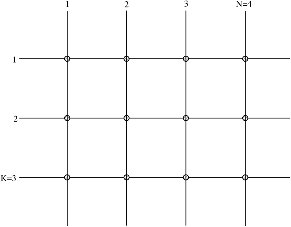
Figure 1: (a) A vertex configuration. (b) Numbering of the lattice.

A statistical weight $w(legs_{i,j};i,j)=\exp{[-\beta~{}\varepsilon(legs_{i,j};i,j)]}$ is assigned to each vertex, depending on the legs configurations ($legs_{i,j}=\{h_{i,j},h_{i+1,j},v_{i,j},v_{i,j+1}\}$) around it. If the weight depends explicitly on the position of the vertex, we have a disordered model. The goal is to find the partition function $Z=\sum_{\{legs\}}\prod_{i,j}w(legs_{i,j};i,j)$.

To each vertex, one can associate a matrix, whose elements are the weights corresponding to the possible configurations of legs, in the following way: fix the horizontal legs around site $(i,j)$ to their minimal values, say $h_{i,j}=h_{i+1,j}=1$; then vary the values of the vertical legs, associating the upper one to a row, and the lower one to a column; a $(V_{j}\times V_{j})$ matrix is thus obtained, which we indicate by $L_{j}^{1,1}(i)$, whose entries are the weights corresponding to the possible legs configurations with horizontal legs fixed to 1; then repeat the procedure changing the values of the horizontal legs, associating the left one to a row, and the right one to a column; a block matrix $L_{j}(i)$ is finally obtained, which is conventionally called the Lax operator. It is a $(H_{i}\times H_{i})$ matrix whose entries $L_{j}^{h_{i,j},h_{i+1,j}}(i)$ are in turn $(V_{j}\times V_{j})$ matrices, i.e. operators over the linear space ${\mathcal{H}}_{j}$. The partition function of the $(1\times N)$ lattice with periodic boundary conditions in vertical and horizontal direction is, in terms of the Lax operators, $Z_{1}=\text{Tr}_{V}\text{Tr}_{H}\{L_{1}(1)\dotsm L_{N}(1)\}\equiv\text{Tr}_{V}\hat{t}(1)$, where by $\text{Tr}_{H}$ we mean the trace over the horizontal space, and by $\text{Tr}_{V}$ the trace over the vertical ones; we introduced the transfer matrix $\hat{t}(i)\equiv\text{Tr}_{H}\{L_{1}(i)\dotsm L_{N}(i)\}$, where the hat is meant to remind that the transfer matrix is an operator over $\mathcal{H}=\bigotimes_{j}{\mathcal{H}}_{j}$, the direct product of the linear spaces associated to the vertical legs. For a $(K\times N)$ lattice, the partition function is $Z=\text{Tr}_{V}\{\hat{t}(1)\dots\hat{t}(K)\}$. If $[\hat{t}(i),\hat{t}(i^{\prime})]=0$ $\forall i,i^{\prime}$, it is possible to simultaneously diagonalize the $\hat{t}(i)$, obtaining $Z=\sum_{r}\prod_{i=1}^{K}t_{r}(i)$, where $t_{r}(i)$ is the $r$-th eigenvalue of $\hat{t}(i)$. In this case, the VM is exactly solvable.
From the $\hat{t}(i)$, it is commonly possible to extract many-body Hamiltonians of interest. Thus, a given exactly solvable vertex model corresponds uniquely to a family of commuting many-body operators.
It turns out that the transfer matrices commute with each other, and thus the corresponding vertex model is exactly solvable, if $H_{i}=H_{i^{\prime}}=H$, $\forall i,i^{\prime}$, and a family of $(H^{2}\times H^{2})$ matrices, the $\check{R}$-matrices, exists, such that the Lax operators obey the relation

$$\check{R}(i,i^{\prime})~{}L_{j}(i)\otimes L_{j}(i^{\prime})=L_{j}(i^{\prime})\otimes L_{j}(i)~{}\check{R}(i,i^{\prime})\;.$$ (50)

Given a $\check{R}$-matrix, this is a very strict requirement, which in general implies that many legs configurations are not allowed, i.e. their weight is zero, while the allowed ones are related to each other by some parametrization.

A relevant case is when the dimensions of vertical and horizontal space are equal, and they do not depend on the row or column: $H_{i}=V_{j}\equiv 2S+1$. Then, the $\check{R}$-matrices are but the Lax operators where the matrix elements have been written down explicitly in their matrix representation. It turns out that the entries of the Lax operators are matrices belonging to the $(2S+1)$-dimensional realization of $su(2)$, i.e. spins over the Hilbert space ${\mathcal{H}}_{j}$. There is the drawback that the $\check{R}$-matrix is difficult to determine and to handle, since its dimension increases very fast with $S$ [29, 30]. A technique to build larger $\check{R}$-matrices using the $(4\times 4)$ $\check{R}$-matrices (the simplest ones) as building blocks was devised by Kulish, Reshetikhin, and Sklyanin [31]. In the present paper, by means of the quasi-classical expansion, we will build up operators for spins higher than $1/2$ still making use of $(4\times 4)$ $\check{R}$-matrices.

Appendix B General $K_{+}$ matrix

In this appendix we construct the Hamiltonian when the general solution of the reflection equation (15) is considered [33, 34]. In this case we have

$$K_{+}(u)=\frac{1}{p}\left(\begin{matrix}\sinh[p(u+\eta+\xi_{+})]\quad&\kappa_{+}\sinh[2p(u+\eta)]\\ \kappa_{+}\sinh[2p(u+\eta)]\quad&-\sinh[p(u+\eta-\xi_{+})]\quad\end{matrix}\right)\;.$$ (51)

Since we want $\hat{\tau}^{(1)}$ to be a  C-number, we must impose $\kappa_{+}\simeq i\eta c$. Thus, the final effect of the general reflection results in an additional term in the second order of the transfer matrix

$$\begin{split}&\hat{\tau}^{(2)}(u)\to\hat{\tau}^{(2)}(u)+\frac{2ic}{p}P(u)P^{-1}(-u)\sinh^{2}{(2pu)}\Biggl{\{}\\ &\sum_{j}\frac{\sinh[p(z_{j}-\xi)]}{\cosh(2pu)-\cosh(2pz_{j})}\hat{S}_{j}^{+}-\sum_{j}\frac{\sinh[p(z_{j}+\xi)]}{\cosh(2pu)-\cosh(2pz_{j})}\hat{S}_{j}^{-}\Biggr{\}}\;.\end{split}$$ (52)

The Hamiltonian is again built according to

$$H=\sum_{j}2h_{j}\hat{\tau}_{j}$$ (53)

where the integrals of motion are

$$\begin{split}\hat{\tau}_{j}=&~{}(1-J\,\hat{S}^{z})\hat{S}_{j}^{z}-ic\,J\left(\frac{\sinh[p(z_{j}-\xi)]}{p}\hat{S}_{j}^{+}-\frac{\sinh[p(z_{j}+\xi)]}{p}\hat{S}_{j}^{-}\right)+\\ &-J\sum_{\genfrac{}{}{0.0pt}{}{k}{k\neq j}}\frac{1}{\cosh(2pz_{j})-\cosh(2pz_{k})}\Biggl{[}\\ &\phantom{\mbox{ }+}\bigl{(}\cosh(2pz_{j})+\cosh(2pz_{k})-2\cosh(2p\xi)\bigr{)}\hat{S}_{j}^{z}\hat{S}_{k}^{z}+\\ &+\bigl{(}{\cosh[p(z_{j}+z_{k})]-\cosh(2p\xi)\cosh[p(z_{j}-z_{k})]}\bigr{)}\left(\hat{S}_{j}^{+}\hat{S}_{k}^{-}+\hat{S}_{j}^{-}\hat{S}_{k}^{+}\right)+\\ &-{\sinh(2p\xi)\sinh[p(z_{j}-z_{k})]}\left(\hat{S}_{j}^{+}\hat{S}_{k}^{-}-\hat{S}_{j}^{-}\hat{S}_{k}^{+}\right)\Biggr{]}\;.\end{split}$$ (54)

We point out that the Hamiltonian is hermitian for real $c$ and $\xi=it$ with real $t$. The diagonalization of this class of Hamiltonians might be achieved by functional Bethe ansatz[6]. Nevertheless, it seems worth to study the models (53), (54) since their potential application to condensed matter (see also Eqs (43), (44)).

Appendix C Generalization to $su(n)$

In this appendix we briefly discuss on a generalization of the Gaudin model to the $su(n)$ case. We can define the Gaudin model for other Lie algebras (see, e.g., Ref. [32] for recent works). Following the method depicted in section 3 we obtain a modified Gaudin Hamiltonian to include a scalable term proportional to the Cartan generators of $su(n)$ (as far as we know, previously obtained models do not contain this term).

The trigonometric $R$-matrix for $su(n)$ chains is given by

$$R(\lambda)=\frac{1}{p}\sum_{a=1}^{n}\sinh(p(\lambda+\eta))E^{aa}\otimes E^{aa}+\frac{1}{p}\sum_{a\neq b}^{n}\sinh(p\lambda)E^{aa}\otimes E^{bb}\\ +\frac{1}{p}\sum_{a\neq b}^{n}e^{-p\lambda{\rm sgn}(a-b)}\sinh(p\eta)E^{ab}\otimes E^{ba},$$ (55)

where $E^{ab}$ denotes $n\times n$ matrix with unity at $(a,b)$ element. They satisfy

$$[\hat{E}^{ab},\hat{E}^{cd}]=\Bigl{(}\delta^{bc}\hat{E}^{ad}-\delta^{da}\hat{E}^{cb}\Bigr{)}.$$

The corresponding diagonal solution of the reflection equation (14) is [33]

$$K_{-}(\lambda) =\frac{1}{p}\sum_{a=1}^{\ell_{-}}e^{p\lambda}\sinh(p(\xi_{-}-\lambda))E^{aa}+\frac{1}{p}\sum_{a=\ell_{-}+1}^{n}e^{-p\lambda}\sinh(p(\xi_{-}+\lambda))E^{aa},$$

$$K_{+}(\lambda) =\frac{1}{p}\sum_{a=1}^{\ell_{+}}e^{-p\lambda-2p\eta a}\sinh(p(\xi_{+}+\lambda))E^{aa}$$

$$\qquad+\frac{1}{p}\sum_{a=\ell_{+}+1}^{n}e^{p\lambda+p\eta(n-2a)}\sinh(p(\xi_{+}-\eta n-\lambda))E^{aa}$$ (56)

where $\ell_{\pm}$ is arbitrary, $1\leq\ell_{\pm}\leq n$. Hereafter we set $\ell_{+}=\ell_{-}=\ell$ for simplicity. With these $K$-matrices, the Hamiltonian of the $su(n)$ homogenous spin chain with nearest neighbour interaction with open boundary was computed in Refs. [35, 36] by using the formula (20). The Hamiltonian with the long range interaction is constructed following the procedure presented in section 3.4, where the constants of motion are calculated by the formula (21). They read

$$\hat{\tau}_{j}=2\sum_{a=1}^{n}a\hat{E}_{j}^{aa}\\ +\sum_{a=1}^{\ell}\biggl{[}\xi_{-}^{(1)}\coth(p(\xi-z_{j}))+\xi_{+}^{(1)}\coth(p(\xi+z_{j}))+(n-\ell)\frac{\sinh(2pz_{j})}{\sinh(p(\xi-z_{j}))\sinh(p(\xi+z_{j}))}\biggr{]}\hat{E}_{j}^{aa}\\ +\sum_{a=\ell+1}^{n}\biggl{[}\xi_{-}^{(1)}\coth(p(\xi+z_{j}))+\xi_{+}^{(1)}\coth(p(\xi-z_{j}))\biggr{]}\hat{E}_{j}^{aa}\\ +\sum_{k\neq j}\Biggl{[}\bigl{(}\coth(p(z_{j}-z_{k}))+\coth(p(z_{j}+z_{k}))\bigr{)}\sum_{a}^{n}\hat{E}_{j}^{aa}\hat{E}_{k}^{aa}\\ +\sum_{a\neq b}^{n}\frac{e^{p(z_{j}-z_{k}){\rm sgn}(a-b)}}{\sinh(p(z_{j}-z_{k}))}\hat{E}_{j}^{ba}\hat{E}_{k}^{ab}+\sum_{a=1}^{\ell}\sum_{b=\ell+1}^{n}\frac{\sinh(p(\xi+z_{j}))}{\sinh(p(\xi-z_{j}))}\frac{e^{p(z_{k}-z_{j})}}{\sinh(p(z_{j}+z_{k}))}\hat{E}_{j}^{ba}\hat{E}_{k}^{ab}\\ +\sum_{a=\ell+1}^{n}\sum_{b=1}^{\ell}\frac{\sinh(p(\xi-z_{j}))}{\sinh(p(\xi+z_{j}))}\frac{e^{p(z_{j}-z_{k})}}{\sinh(p(z_{j}+z_{k}))}\hat{E}_{j}^{ba}\hat{E}_{k}^{ab}\\ +\sum_{\begin{subarray}{c}a,b=1\\ a\neq b\end{subarray}}^{\ell}\frac{e^{p(z_{j}+z_{k}){\rm sgn}(b-a)}}{\sinh(p(z_{j}+z_{k}))}\hat{E}_{j}^{ba}\hat{E}_{k}^{ab}+\sum_{\begin{subarray}{c}a,b=\ell+1\\ a\neq b\end{subarray}}^{n}\frac{e^{p(z_{j}+z_{k}){\rm sgn}(b-a)}}{\sinh(p(z_{j}+z_{k}))}\hat{E}_{j}^{ba}\hat{E}_{k}^{ab}\Biggr{]}$$ (57)

where $\hat{E}_{k}^{ab}$ are site-$k$ $su(n)$ operators.

The spectrum of $\hat{\tau}_{j}$ is given as limit of the eigenvalues of the $su(n)$-transfer matrix (Eq.(6) of [35]) and with $u\to z_{j}$:

$$\tau_{j}=\xi_{+}^{(1)}\,\Bigl{(}\coth[p(z_{j}+\xi)]-\coth(p\xi)\Bigr{)}-\xi_{-}^{(1)}\,\Bigl{(}\coth[p(z_{j}+\xi)]+\coth(p\xi)\Bigr{)}\\ +(\ell-n)\frac{\sinh(2pz_{j})}{\sinh[p(z_{j}-\xi)]\sinh[p(z_{j}+\xi)]}+1-n\frac{e^{-2z_{j}}}{\sinh(2z_{j})}\\ +\sum_{k\neq j}^{N}\Bigl{(}\coth[p(z_{j}+z_{k})]+\coth[p(z_{j}-z_{k})]\Bigr{)}\\ \hskip 142.26378pt+\sum_{k}^{M_{1}}\Bigl{(}\coth[p(z_{j}+e_{k}^{(1)})]+\coth[p(z_{j}-e_{k}^{(1)})]\Bigr{)}$$ (58)

The Bethe ansatz equations can be obtained in the same limit of a result in Ref. [35] , and we have (for $a=1,2,\dots,n-1$)

$$2\sum_{k\neq j}^{M_{a}}\Bigl{(}\coth[p(e_{j}^{(a)}+e_{k}^{(a)})]+\coth[p(e_{j}^{(a)}-e_{k}^{(a)})]\Bigr{)}\\ +\delta_{a,\ell}\,\Bigl{(}n+\xi_{-}^{(1)}-\xi_{+}^{(1)}\Bigr{)}\,\Bigl{(}\coth[p(z-\xi)]+\coth[p(z+\xi)]\Bigr{)}\\ =\sum_{k}^{M_{a+1}}\Bigl{(}\coth[p(e_{j}^{(a)}+e_{k}^{(a+1)})]+\coth[p(e_{j}^{(a)}-e_{k}^{(a+1)})]\Bigr{)}\\ +\sum_{k}^{M_{a-1}}\Bigl{(}\coth[p(e_{j}^{(a)}+e_{k}^{(a-1)})]+\coth[p(e_{j}^{(a)}-e_{k}^{(a-1)})]\Bigr{)}$$ (59)

Here we assume $e_{j}^{(0)}=z_{j}$ and $M_{0}=N$, $M_{n}=0$.

The fermionic models can be obtained by using the fermionic realization

$$\hat{E}^{ab}_{j}=c_{j,a}^{\dagger}\,c_{j,b}-\frac{1}{n}\,\delta_{ab},$$ (60)

with a constraint

$$\sum_{a}c_{j,a}^{\dagger}\,c_{j,a}=1.$$

References

[1]
R. J. Baxter.
Exactly Solved Models in Statistical Mechanics.
Academic Press (1982).
[2]
M. Gaudin.
La fonction d’onde de Bethe.
Masson (1983).
[3]
V. E. Korepin, N. M. Bogoliubov, and A. G. Izergin.
Quantum Inverse Scattering Method and Correlation Functions.
Cambridge Univ. Press (1993).
[4]
M. Gaudin,
J. Physique 37, 1087 (1976).
[5]
K. Hikami, P. P. Kulish, and M. Wadati,
J. Phys. Soc. Jpn 61, 3071 (1992).
[6]
E. K. Sklyanin, J. Sov. Math. 47, 2473 (1989).
[7]
M. C. Cambiaggio, A. M. F. Rivas, and M. Saraceno,
Nucl. Phys. A 624, 157 (1997).
[8]
R. W. Richardson,
Phys. Lett. 3, 277 (1963).
[9]
J. von Delft and D. C. Ralph,
Physics Reports 345, 61 (2001).
[10]
A. Mastellone, G. Falci, and R. Fazio,
Phys. Rev. Lett. 80, 4542 (1998).
[11]
L. Amico, G. Falci, and R. Fazio,
J. Phys. A 34, 6425–6434 (2001).
[12]
G. Sierra,
Nucl. Phys. B 572, 517–534 (2000).
[13]
H. M. Babujian, J. Phys. A 26, 6981 (1993).
[14]
N. Reshetikhin and A. Varchenko.
In Geometry, Topology, and Physics, page 293 (1995).
[15]
L. Amico, A. Di Lorenzo, and A. Osterloh,
Phys. Rev. Lett. 86, 5759 (2001).
[16]
L. Amico, A. Di Lorenzo, and A. Osterloh,
Nucl. Phys. B 614, 449 (2001).
[17]
J. Dukelsky, C. Esebbag, and P. Schuck,
Phys. Rev. Lett. 87, 66403 (2001).
[18]
J. von Delft and R. Poghossian,
Algebraic Bethe Ansatz for a discrete-state BCS pairing model, cond-mat/0106405.
[19]
E. K. Sklyanin,
J. Phys. A 21, 2375 (1988).
[20]
K. Hikami,
J. Phys. A 28, 4997 (1995).
[21]
K. Hikami, J. Phys. A 28, 4053 (1995).
[22]
I. Cherednik, Theor. Math. Phys. 61, 35 (1984).
[23]
H. J. de Vega,
Nucl. Phys. B 240, 495 (1984).
[24]
H. M. Babujian,
Phys. Lett. A 90, 479 (1982).
[25]
L. A. Takhtajan,
Phys. Lett. A 87, 479 (1982).
[26]
L. Amico, A. Di Lorenzo, A. Mastellone, A. Osterloh, and R. Raimondi,
Annals of Physics 299, 228 (2002).
[27]
A. Di Lorenzo,
A new class of exactly solvable models.
PhD thesis, Università di Catania, Italy, (2001).
[28]
R.W. Richardson.
private communication.
[29]
V.I. Fateev and A.B. Zamolodchikov, Sov. J. Nucl. Phys. 32, 298 (1980).
[30]
K. Sogo, Y. Akutsu, and T. Abe, Prog. Theor. Phys. 70, 730 (1983).
[31]
P.P. Kulish, N. Reshetikhin, and E.K. Sklyanin, Lett. Math. Phys. 5, 393
(1981).
[32]
P. P. Kulish and N. Manojlovic,
Lett. Math. Phys. 55, 77 (2001).
[33]
H. J. de Vega and A. Gonzalez-Ruiz, J. Phys. A 26, L519 (1993).
[34]
S. Ghoshal and A. Zamolodchikov, Int. J. Mod. Phys. A 9, 3841
(1994).
[35]
H. J. de Vega and A. González-Ruiz,
Mod. Phys. Lett. A 9, 2207 (1994).
[36]
A. Doikou and R. I. Nepomechie,
Nucl. Phys. B 530, 641 (1998).