Two-dimensional Packing in Prolate Granular Materials

Abstract

We investigate the two-dimensional packing of extremely prolate (aspect ratio $\alpha=L/D>10$) granular materials, comparing experiments with Monte-Carlo simulations. In experimental piles of particles with aspect ratio $\alpha=12$ we find the average packing fraction to be $0.68\pm 0.03$. Both experimental and simulated piles contain a large number of horizontal particles, and particle alignment is quantified by an orientational order correlation function. In both simulation and experiment the correlation between particle orientation decays after a distance of two particle lengths. It is possible to identify voids in the pile with sizes ranging over two orders of magnitude. The experimental void distribution function is a power law with exponent $-\beta=-2.37\pm 0.05$. Void distributions in simulated piles do not decay as a power law, but do show a broad tail. We extend the simulation to investigate the scaling at very large aspect ratios. A geometric argument predicts the pile number density to scale as $\alpha^{-2}$. Simulations do indeed scale this way, but particle alignment complicates the picture, and the actual number densities are quite a bit larger than predicted.

I Introduction

One of the more striking features of piles of very prolate granular materials (large aspect ratio $\alpha=L/D$) is the connected network that forms at comparatively low packing fractions. The formation of this network is often commercially undesirable. LCD screens, for example, cannot function if the molecules are entangled, and lumber floating down a river stops when the logs jam. There are, however, practical applications for such “jammed” networks. Piles of large aspect-ratio materials are extremely rigid, even at low packing fractions, and have a high strength:weight ratio. At the extremely small scale, networks of carbon nanotubes are a possible mechanism for conducting energy to and from nano-devices Raffaelle et al. (2001).

Little is known about even basic characteristics of piles formed from rod-like particles, most research on non-spherical particles, whether in twoBuchalter and Bradley (1992a, b); Williams and Mustoe (1990); Mustoe et al. (2000); Cleary and Sawley (2002); Rankenburg and Zieve (2001) or three Villarruel et al. (2000) dimensions, being limited to $\alpha<5$. The rigidity of such piles is due to particle entanglement, with particle rotation extremely constrained. The statistics of particle orientations which determine these constraints, however, is not known. While it seems obvious that particles will align, in fact two-dimensional piles contain a number of orthogonal particles that create large voids which dominate the pile landscape (see Fig. 1). The only work above $\alpha\sim 10$ we are aware of is that of Philipse Philipse (1996); Philipse and Verberkmoes (1997), who formed three-dimensional piles of copper wire of aspect ratios ranging from 5 to 77 and explained the $1/\alpha$ scaling of the volume fraction with a simple geometric model. As the particles’ aspect ratio increased, they could no longer be poured from their initial container, and tended to fall out as a solid “plug”. The cause of this transition, which occurs at $\alpha\sim 35$, is not known.

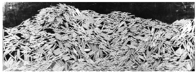
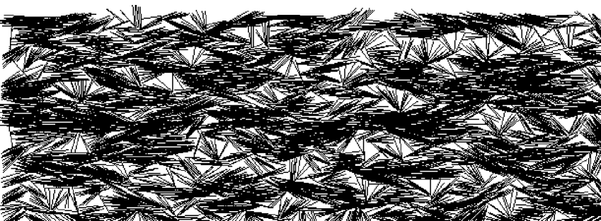
Figure 1: Top: 2-d pile of $\alpha=12$ acrylic rods backlit with fluorescent lights. The middle third of each particle appears bright. Bottom: Simulated pile of $\alpha=12$ particles. Both piles show particles aligning and a wide distribution of void sizes.

II Experiment and Simulation

To form prolate particles, acrylic rods (diameter $D=0.16$ cm) were cut to a length $L=1.9$ cm ($\alpha\approx 12$) and constrained between two Plexiglas sheets separated by a spacer 1.25 particle diameters thick. The uniform spacing throughout the plates prevents particles from overlapping; piles are effectively 2-dimensional. Thicker spacers result in overlapping particles which are pinched between the plates and immobile. Whereas Philipse observed a qualitative increase in pile rigidity in three dimensions to occur at about an aspect ratio of 35, we believe that in two dimensions this occurs at much lower aspect ratios. We have observed 2-d piles of particles with aspect ratio 10 to have stable angles of repose of $90^{\circ}$ or greater (see Fig. 2). We associate this behavior in 2-d with Philipse’s solid plug observed in 3-d.

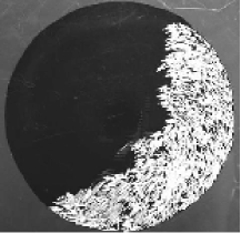
Figure 2: 2-dimensional pile of $\alpha=10$ particles showing an angle of repose of $90^{\circ}$. We believe that the ability to support angles of $90^{\circ}$ or greater is analogous with Philipse’s observation of solid plugs in three dimensions.

Piles are formed by distributing particles at random on one Plexiglas sheet, attaching the second sheet, and slowly rotating the system to vertical. The initial distribution is not truly random; local orientational correlations exist as neighboring particles are forced to be aligned (or else they would overlap). This could be avoided in principle by reducing the number of particles on the plate; in practice, however, this would be prohibitively slow. Additional particles are prepared in a similar manner in an identical cell which is used as a funnel to pour particles onto the pile. Piles formed this way are 53 cm wide, typically 25 cm high and contain about 2000 particles. A picture of a pile is shown in Fig. 1 (top). The piles are backlit with fluorescent lights. The cylindrical rods act as lenses, displaying a thin bright line throughout the middle of each particle. We have written software that identifies connected, collinear bright pixels in a picture and extracts the particle location and orientation. Data reported involve averaging over 19 separate piles. Despite the less-than-ideal preparation, piles were statistically consistent; packing fractions varied by $\sim 5\%$ and void distribution and orientational order functions were similarly reproducible.

Buchalter and BradleyBuchalter and Bradley (1992a, b) developed a Monte-Carlo simulation for ellipsoidal particles. We adapted this for cylindrical particles and extended the aspect ratio by two orders of magnitude ($\alpha_{\rm max}=1000$). Particles move along the nodes of a discrete lattice ($N\times N$, with $N\sim 10L$) and can rotate freely. Particles are initially placed at random locations on the lattice and given random orientations (never being allowed to overlap with other particles). A single particle is chosen at random and moved along a randomly generated displacement/rotation path. The only constraint on the motion is that particles cannot move upwards or overlap with other particles. The maximum possible distance a particle can move in one attempt is typically $L/6$. If an intersection occurs, the particle is placed at its last allowable position and a new particle is then chosen for an attempted move. At any given time, only one particle is in motion. The process repeats until the potential energy (the sum of the particle heights) remains constant for 5000 time steps, each particle unable to move for, on average, 10 attempted moves. A new group of particles is then placed above the formed pile and allowed to settle. All piles are at least 7 particle lengths high and we have checked to ensure that additional pourings do not appreciably change the pile’s statistics. A sample pile is shown in Fig. 1 (bottom). The length of the particles, constant through any one pile, is varied from 10 to 1000. Results for a given aspect ratio are averaged over five piles; additional piles do not change the statistics. Additional details about the simulation’s validity, including a discussion comparing the simulation in the limit as the aspect ratio goes to 1 with experimental findings, can be found in Buchalter and Bradley (1992a).

III Results

III.1 Global Pile Characteristics

The range of packing fractions achievable with 2-d disks under gravitational forces is quite narrow. The upper and lower limits are given by hexagonal ($\phi_{hcp}=\pi/(2\sqrt{3})\approx 0.907$) and orthgonal ($\phi_{ocp}=\pi/4\approx 0.785$) close packing respectively, with a random close packing vale of $\phi_{rcp}\approx 0.82$Howell and Behringer (1999). We find the average packing fraction of rods with $\alpha=12$ to be $\phi=0.68\pm 0.03$. The lowest measured value was 0.63; the largest 0.72.

The orientational order parameter $Q=\langle\cos(2\theta_{i})\rangle$ is used to characterize the angular distribution of particles. $\theta_{i}$ is the angle with respect to the horizontal of the $i$-th particle and the average is over all particles. $Q$ takes values ranging from $-1$ (all vertical) to $+1$ (all horizontal), with $Q=0$ indicating an isotropic distribution of angles (or all angles equal to $45^{\circ}$). For the experimental piles $Q=0.33\pm 0.05$; simulated piles have similar values regardless of aspect ratio.

Figure 3 shows the distribution of particle angles in experimental and simulated piles. Both have a peak around $\theta=0$, indicating a preference for horizontal orientation; this preference is stronger in the simulated pile.

Figure 3: Angular distribution of experimental ($\bullet$) and simulated ($\ast$) particles. Both show a peak about horizontal alignment ($\theta=0$), the experiment having the broader distribution.

To determine whether this ordering was caused by the flat bottom boundary, we calculated the orientational order parameter for all particles whose centers of mass are at height $h$. We denote this height dependent value as $Q_{h}(h)$. A plot of $Q_{h}(h)$ vs. height for experimental piles is shown in Fig. 4. $Q_{h}(h=0)$ is 1, as particles on the floor must be horizontal. At a height of $h=L$, however, $Q_{h}(h)$ has already decayed significantly. For heights greater than a particle length, $Q_{h}(h)$ fluctuates about an average value. From this we infer that the bottom boundary’s influence on particle orientation does not extend beyond one particle length. Simulations show a similar asymptotic value for $Q_{h}(h)$, and it should be noted that the bottom boundary in the simulations does not impose a horizontal angle on the bottom particles. Therefore we believe the tendency for particles to be horizontal, more pronounced the simulation than in the experiment, is a result of gravity (in the simulation imposed by the restriction that particles cannot move upwards) rather than a boundary condition.

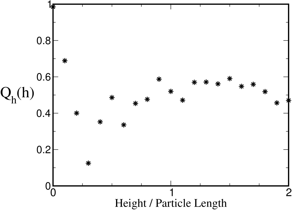
Figure 4: Orientational order parameter $Q_{h}(h)$ as function of height in pile. The reaching of an asymptotic value so quickly (for $h\sim L$) indicates that the bottom boundary is not significantly influencing the orientation of particles high up in the pile. Simulations, which do not have a horizontal bottom boundary but rather allow the bottom particles to assume any angle, show a similar average $Q_{h}(h)$ at all heights.

Experimental piles also have more vertical particles than the simulation, a consequence, we believe, of friction between particles which is not incorporated in the simulation.

III.2 Distribution of Voids

The appearance of both simulated and experimental piles are dominated by large, but rare, voids. From the images we find the number of voids as a function of void area $A$. The void distribution functions $V(A)$ from experimental ($\bullet$) and simulated ($\ast$) piles are plotted vs. void area $A$ in Fig. 5. As Fig. 5 shows, experimental void sizes vary by over two decades. The experimental data are well-fit by a power law $A^{-2.37\pm 0.05}$ (straight line in Fig. 5).

Figure 5: Void distribution function $V(A)$ as a function of void area scaled by particle length $L$ squared. $V(A)$ is expressed as a percentage of the total number of voids. Voids in both experiment ($\bullet$) and simulation ($\ast$, with $\alpha=20$) decay as a $A^{-\beta}$ with $\beta=2.37\pm 0.05$. This means that smaller voids occupy a greater total area than the larger, rarer, voids.

Simulated piles show a similar decay, although the function does not seem to follow a power law. We did not notice any significant dependence of the void distribution function on the particle aspect ratio in simulated piles, although this warrants further study.

There are several intriguing consequences to the fact that the exponent in $V(A)$ is between -2 and -3. First, the total area taken up by all voids with size $A$ is $AV(A)\propto A^{-1.37}$. As $\lim_{A\rightarrow\infty}[AV(A)]\rightarrow 0$, the cumulative effect of the smaller voids to the pile’s area is actually larger than that of the larger voids. We also note that the total area occupied by all voids $\int{AV(A){\rm d}A}$ remains finite as, in fact, it must for realistic piles. The total area occupied by voids is related to the packing fraction $\phi$ by the relation

$$\int{AV(A){\rm d}A}=\int{A^{-1.37}{\rm d}A}=A_{\rm tot}(1-\phi),$$

where $A_{\rm tot}$ is the total pile area. This relation can be used to explore the lower limits for the void size, without which the integral on the left diverges. This is the subject of current research. We also note that the absence of an upper limit for void size results in the divergence of the integral for the mean square void area $\langle A^{2}\rangle=\int{V(A)A^{2}{\rm d}A}$.

III.3 Neighboring Particle Alignment

Both experiment and simulation find neighboring particles aligning. This is quantified with an orientational correlation function

$$\tilde{Q}(r)=\langle\cos{(2\Delta\theta_{ij})}\rangle.$$

$\Delta\theta_{ij}$ is the difference in angle between particles $i$ and $j$ and the average is over all particles whose centers-of-mass separation is between $r$ and $r+\delta r$. This function, related to an earlier orientational order parameter Buchalter and Bradley (1992a, b), takes values ranging from 1 if particles are parallel to -1 if particles are perpendicular. Two particles whose centers-of-mass are quite close must be aligned and so $\tilde{Q}(r\rightarrow 0)\rightarrow 1$. Once particle centers-of-mass are separated by more than one particle length $L$ they can in principle assume any relative orientation and so $\tilde{Q}(r\rightarrow\infty)\rightarrow 0$. For comparison, we calculate analytically the correlation function resulting from a distribution where particless assume all allowable angles with equal probability. This is the simplest possible ordering, the only constraint being that particles cannot overlap, and is used in simple geometric models for predicting number density. The allowable angles $\theta$ a particle can take with respect to a fixed particle assumed to lie along the $x$ axis are found as a function of center-of-mass separation $r$ and angle $\phi$ that the line connecting the centers-of-mass makes with the $x$ axis. If the minimum/maximum allowable angles are given by $\theta_{min}$ and $\theta_{max}$ then $\tilde{Q}(r)$ is

$$\tilde{Q}(r)=\int_{0}^{2\pi}{\rm d}\phi\int_{\theta_{min}(r,\phi)}^{\theta_{max}(r,\phi)}\cos{(2\theta)}{\rm d}\theta.$$

Figure 6 shows the $\tilde{Q}(r)$ distribution resulting from the analytic (line), experimental ($\bullet$), and simulated ($\ast$) piles. Both the experimental and simulated piles show greater correlation between neighboring particles, seen in the divergence from the analytic line for $r/L>0.5$ (between the dashed lines), and reach an asymptotic value once particles are separated by more than two particle lengths.

The long-range correlation between particles shown in Fig. 6 does not represent a long-range influence of one particle on another, but rather results from the overall preference for particles to be horizontal. This is confirmed by calculating

$$\tilde{Q}(r\rightarrow\infty)=\int P(\theta)P(\phi)\cos{[2(\theta-\phi)]}{\rm d}\theta{\rm d}\phi,$$

which assumes the particle angles are drawn at random from the distribution $P(\theta)$ shown in Fig. 3. The differences in the simulation and experimental distribution functions result in $\tilde{Q}_{\infty}^{\rm exp}=0.16$ and $\tilde{Q}_{\infty}^{\rm sim}=0.53$, agreeing quite well with the asymptotic values in Fig. 6.

Figure 6: Orientational correlation function $\tilde{Q}(r/L)$ as a function of center-of-mass separation scaled by particle length. The solid line represents the correlation resulting from a distribution where particles assume all allowable angles with equal probability. Both experiment and simulation show enhanced alignment for $r/L$ between 0.5 and 1 (between dashed lines) but noticeably different asymptotic values due to the different angular distributions from Fig. 3.

$\tilde{Q}(r/L)$ reaches its asymptotic value for both simulation and experiment within two particle lengths. This correlation length is the same for simulations of particle lengths differing by two orders of magnitude, as shown in Fig. 7. The curves in Figure 7 have all been normalized by their asymptotic value; that is, what is plotted is $(\tilde{Q}-\tilde{Q}_{\infty})/(1-\tilde{Q}_{\infty})$, which takes values ranging from 1 to 0. When thus normalized, all simulated curves lie very close to the experimental curve.

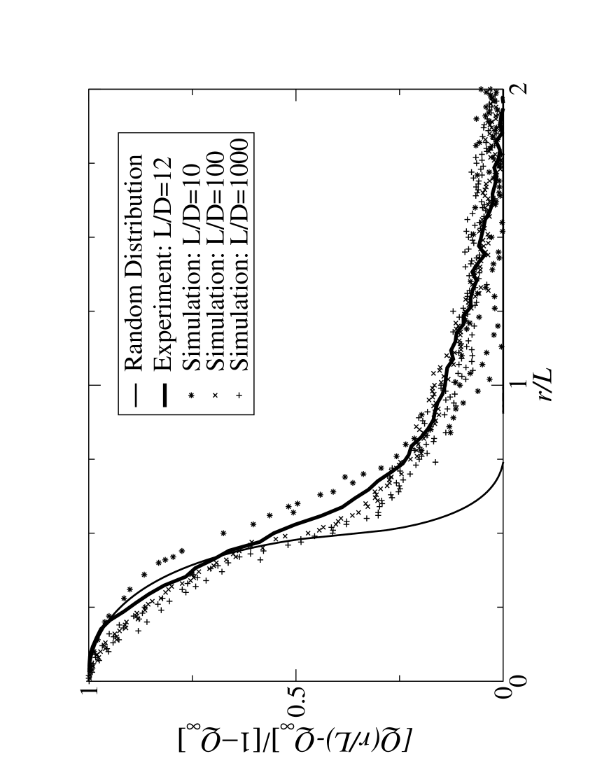
Figure 7: Orientational correlation function $\tilde{Q}(r/L)$ normalized by the asymptotic value $\tilde{Q}_{\infty}$ as a function of center-of-mass separation scaled by particle length. Simulation results are shown for particle lenghts varying over three orders of magnitude; the correlation length at which the asymptotic value is reached is the same for simulations and experiment.

III.4 Simulation at Large Aspect Ratios

We now extend the simulation to larger aspect ratios and investigate the scaling of various quantities. The rigidity of a pile depends on particles in contact, hence we calculate the contact number $\langle c\rangle$. Fig. 8(top) shows that $\langle c\rangle$ reaches an asymptotic value of $\approx 3.2$ by aspect ratio 50. This may seem counter-intuitive, as longer particles in principle can be in contact with more neighbors. Orientations that maximize $\langle c\rangle$, however, are quite rare and the length-independence of contact number is due to the tendency of neighboring particles to align and screen one another from other particles. As particle aspect ratio decreases, and the particles become more circular, this screening effect diminishes and the contact number increases. Packings of circular disks, for example, show a contact number between 4 (orthogonal close packing) and 6 (hexagonal close packing).

Recall that the pile’s orientational order is characterized by the order parameter $Q=\langle\cos(2\theta_{i})\rangle$ where $\theta_{i}$ is the angle the $i$th particle makes with the horizontal and $Q$ is averaged over all particles. As shown in Fig. 8, $Q$ of simulated piles decreases as the particle length increases reaching an asymptote of 0.3. $Q$ for experimental piles of particles with aspect ratio $\alpha=12$ is $0.33\pm 0.05$, comparable with that of of simulations.

Figure 8: Top: Contact number in simulated piles as a function of particle aspect ratio. $\langle c\rangle$ is independent of aspect ratio for long particles, and reaches a suitable asymptote, 4.5, comparable withe contact number of disks, as $\alpha\rightarrow 1$. Bottom: Orientational order parameter $Q$ as a function of aspect ratio for simulation ($\ast$) and experiment ($\bullet$).

III.5 Phenomenology

Philipse gave a simple geometric argument, the Random Contact ModelPhilipse (1996) (RCM)to explain the low packing fractions of three-dimensional piles. We now apply his logic to our two-dimensional piles and show the discrepancies caused by the enhanced particle alignment described above.

The existence of one particle excludes a fraction of the possible orientations, called the excluded area $A_{\rm excl}$, that can be assumed by a second particle. If we assume a connected network, where all particles are in contact with (on average) $\langle c\rangle$ neighbors and that particles assume all allowable orientations with equal probability, then the average number density will be

$$\langle N\rangle=\frac{2\langle c\rangle}{A_{\rm excl}}.$$

The factor of 2 accounts for the fact that each contact involves two particles. We have already shown, however, that the assumption that contacts are uncorrelated, is not satisfied. BalbergBalberg et al. (1984) has calculated the excluded area of a stick with length $L$ and width $W$; to first order $A_{\rm excl}=(2/\pi)L^{2}$. With $\langle c\rangle=3.2$, the number density as a function of aspect ratio $\alpha$ is predicted to be

$$N(L)=\frac{2\langle c\rangle}{(2L^{2}/\pi)}=CL^{-2}$$

with $C=10$. Fig. 9 shows that $N(L)$ does indeed fall off as $L^{-2}$ for large $L$. The constant, however, is larger than that predicted by the RCM (flat line in Fig. 9). Piles are therefore more dense than predicted, implying that the excluded area of particles is about 33% less than that in an isotropic distribution. This is a result of particle alignment, seen earlier in Fig. 6. We also note that the scaling as $\alpha^{-2}$ is realized only for the largest of aspect ratios, while the constancy of contact number occurs much earlier.

Figure 9: Number density as a function of particle length. As predicted by the simple geometric model described in the text, the number density appears to scale as $L^{-2}$ for large $L$. The actual densities however, are larger than that predicted by the model, a consequence of particle alignment.

IV Conclusions

We have presented the first quantitative characterization of two-dimensional piles formed from prolate ($\alpha>10)$ granular materials finding, for example, the packing fraction of particles with aspect ratio $\alpha=12$ to be $0.68\pm 0.03$. Particles separated by less than two particles lengths show a greater orientational correlation than would be found in a random pile; particles separated by more than two lengths are uncorrelated except for the general preference for horizontal alignment imposed by gravity. The void distribution function in experimental piles obeys a power law with exponent $-\beta=2.37\pm 0.05$; Monte-Carlo simulations show similar angular correlations and void distribution functions. Simulations have a greater number of horizontal particles, however, and thus produce piles with larger number densities than found in both experiment and simple geometric models.

We thank E. F. Redish for first questioning the characteristics of pickup sticks and John C. Crocker for calling attention to the work of Philipse. Eric R. Weeks and L. S. Meichle have provided invaluable advice throughout this project. Saul Lapidus and Peter Gee were involved in much of the original setup of the experiment.

References

- Raffaelle et al. (2001) R. P. Raffaelle, T. Gennett, J. Maranchi, P. Kumta, M. J. Heben, A. C. Dillon, and K. C. Jones, in MRS Bulletin Proceedings (Materials Research Society, 2001), vol. 706.
- Villarruel et al. (2000) F. X. Villarruel, B. E. Lauderdale, D. M. Mueth, and H. M. Jaeger, Phys. Rev. E 61, 6914 (2000).
- Buchalter and Bradley (1992a) B. J. Buchalter and R. M. Bradley, J. Phys. A 25, L1219 (1992a).
- Buchalter and Bradley (1992b) B. J. Buchalter and R. M. Bradley, Phys. Rev. A 46, 3046 (1992b).
- Williams and Mustoe (1990) J. R. Williams and G. W. Mustoe, in Computers and Geotechnics (Elsevier Applied Science Publishers Ltd., 1990).
- Mustoe et al. (2000) G. G. W. Mustoe, M. Miyata, and M. Nakagawa., in Finite Elements: Techniques and Developments (Civil-Comp Press, 2000).
- Cleary and Sawley (2002) P. W. Cleary and M. L. Sawley, Applied Mathematical Modeling 26 (2002).
- Rankenburg and Zieve (2001) I. C. Rankenburg and R. J. Zieve, Phys. Rev. E 63, 061303 (2001).
- Philipse (1996) A. Philipse, Langmuir 12, 1127 (1996).
- Philipse and Verberkmoes (1997) A. P. Philipse and A. Verberkmoes, Physica A 235, 186 (1997).
- Howell and Behringer (1999) D. Howell and R. P. Behringer, Phys. Rev. Lett. 82 (1999).
- Balberg et al. (1984) I. Balberg, C. H. Anderson, S. Alexander, and N. Wagner, Phys. Rev. B 30, 3933 (1984).