Tunnelling-charging Hamiltonian of a Cooper pair pump at large $E_{\mathrm{J}}/E_{\mathrm{C}}$:
Modified Hamiltonians and renormalisability

Abstract

The properties of the tunnelling-charging Hamiltonian of a Cooper pair pump are well understood in the regime of weak and intermediate Josephson coupling, i.e. $E_{\mathrm{J}}\lesssim E_{\mathrm{C}}$. Instead of perturbative treatment of charging effects, the present work applies the charge state representation in the the strong coupling case. From the discrete Hamiltonian we construct effective, truncated PDE Hamiltonians and analytically obtain approximate ground-state wave functions and eigenenergies. The validity of the expressions is confirmed by direct comparison against the results of numerical diagonalisation. For uniform arrays, our results converge rapidly and even $\phi$-dependence of the wave function is described reasonably. In the inhomogeneous case we find the Hamiltonian to be parametrically renormalisable. A method for finding inhomogeneous trial wave function is explained. The intertwined connection linking the pumped charge and the Berry’s phase is explained, too. As addendum, we have explicitly validated the ground state ansatz for $\phi=0$ when $N\leq 42$.

I Introduction

Josephson junction devices, e.g. Cooper pair boxes, superconducting single electron transistors (SSET) and Cooper pair pumps, have been extensively studied both theoreticallyAverin (1998); Pekola et al. (1999); Makhlin et al. (1999); Averin (2000); Falci et al. (2000); Pekola and Toppari (2001) and experimentally.Mooij et al. (1999); Nakamura et al. (1999); Orlando et al. (1999); Choi et al. (2001); Bibow et al. (2002) For a recent review, see Ref. Makhlin et al., 2001. Possible applications include at least direct Cooper pair pumping,Pekola et al. (1999) decoherence studies,Pekola and Toppari (2001) related metrological applications,Hassel and Sepp$\ddot{\mathrm{a}}$ (1999) and the use of Cooper pair charge qubits or persistent-current qubits (SQubits) in quantum computation.Averin (1998); Mooij et al. (1999)

The ideal tunnelling-charging Hamiltonian of a Cooper pair pump has been studied in detail in Refs. Pekola et al., 1999; Aunola et al., 2000; Aunola, 2001. Charge transfer due to direct supercurrent and adiabatic pumping due to varying gate voltages have been adequately described when the Josephson coupling is weak or at most comparable to charging effects. The case of strong Josehpson coupling in ideally biased arrays is still relatively unexplored. A single Josephson junction is known to be described by the Mathieu equationAbramowitz and Stegun (1972) in the phase representation. For a superconducting single electron transistor (SSET) the charge state representation is identical to one-dimensional discrete harmonic oscillator and, thus, the Mathieu equation in the island’s phase representation.Eiles and Martinis (1994); Tinkham (1996)

In this paper we first develop a method for obtaining an approximate solution of the Mathieu equation. Later on, we generalise the method for several dimensions and make the required corrections for our model Hamiltonian. In short, starting from the discrete Hamiltonian we construct a modified partial differential equation (PDE) for which a trial solution is obtained. Subsequently, the solution is overlaid as the wave function the discrete Hamiltonian and the result is compared against numerically obtained eigenstate.

In order to sum up the obtained results we state the following: For homogeneous arrays of arbitrary length we find analytical and rapidly converging wave functions and eigenenergies. These expressions are derived from the developed method The case of non-zero phase difference is treated in a fairly satisfactory way. Inhomogeneous arrays are first treated by parametric renormalisation which yields an accurate approximation for the ground state energy. A modification of the original method improves the wave function, but not the asymptotical rate of convergence.

Skeel and HardySkeel and Hardy (2001) have performed analysis on constructing modified Hamiltonian when integrating systems of PDE’s over time, see also Refs. Reich, 1999; Gans and Shalloway, 2000; Hairer and Lubich, 2000. In these works numerical discretisation is approximately counteracted by using a suitable truncation of the modified equations. The principles of the present method are similar, although it is applied on a discrete eigenvalue problem.

This paper is organised as follows. In Sec. II the Hamiltonian is defined and its structure is explained. In Sec. III we find an approximate solution for the Mathieu equation in charge state representation and postulate the generalisation of the method for several coordinates. In Sec. IV homogeneous arrays are examined and explicit trial wave functions for the ground state are constructed. In Sec. V the developed formalism is extended to into account non-zero values of phase difference across the array. In Sec. VI the Hamiltonian is shown to be parametrically renormalisable in the inhomogeneous case. Wave function is also constructed although the accuracy is not as good as in the homogeneous case. Finally, the conclusions are drawn in Sec. VII.

II Constructing the Hamiltonian

A schematic view of the system is shown in Fig. 1. We assume that the gate voltages $V_{\mathrm{g},j}$ are independent and externally operated. The bias voltage across the array, $V_{\mathrm{b}}$, which controls the total phase difference $\phi$ according to $d\phi/dt=-2eV/\hbar$, is assumed to be ideally set to zero. Hence, $\phi$ remains fixed and becomes a good quantum number in proper variables, which have been presented e.g. in Ref. Ingold and Nazarov, 1992. On the other hand, a precise value of $\phi$ means that its conjugate variable $\hat{M}$, the average number of tunnelled Cooper pairs ($\hat{M}:=-i\partial/\partial\phi$), becomes completely undetermined.

In the following, the tunnelling-charging Hamiltonian

$$H=H_{\mathrm{C}}+H_{\mathrm{J}},$$ (1)

is assumed to be the correct description of the microscopic system. The ideal model Hamiltonian simply neglects quasiparticle tunnelling as well as other degrees of freedom. The most important parameters are the (average) Josephson coupling energy $E_{\mathrm{J}}$ and (average) charging energy, defined as $E_{\mathrm{C}}:=(2e)^{2}/(2C)$. These determine “the Josephson-charging ratio” which is denoted by $\varepsilon_{\rm J}:=E_{\mathrm{J}}/E_{\mathrm{C}}$. The Hamiltonian and the operation of a Cooper pair pump in the weak coupling regime is further determined by (normalised) gate charges $\vec{q}:=\{q_{1},\ldots,q_{N-1}\}$, where $q_{k}:=-C_{{\rm g},k}V_{{\rm g},k}/2e$. In the present model relative junction capacitances $\vec{c}$, where $c_{k}:=C_{k}/C$ and $\sum_{k=1}^{N}C_{k}^{-1}=N/C$, also determine individual Josephson energies by $E_{\mathrm{J},k}:=c_{k}E_{\mathrm{J}}$. For uniform or homogeneous arrays we have $c_{k}:=1$, while the inhomogeneity can be reliably quantified by the inhomogeneity index $X_{\rm inh}:=[\sum_{k}(c_{k}^{-1}-1)^{2}/N]^{1/2}$.Aunola et al. (2000); Aunola (2001)

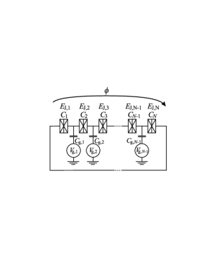
Figure 1: An ideal superconducting array of independent Josephson junctions. Here $C_{k}$ and $E_{\mathrm{J},k}$ are the capacitance and the Josephson energy of the $k^{\mathrm{th}}$ junction, respectively. The total phase difference across the array, $\phi$, is a constant of motion.

The matrix elements of the charging Hamiltonian $H_{\rm C}$ are given by the capacitive charging energy and thus they readAunola et al. (2000)

$$\langle\vec{n}|H_{\rm C}(\vec{q})|\vec{n}\rangle_{\phi}=E_{\rm C}\left[\sum_{k=1}^{N}\frac{v_{k}^{2}}{c_{k}}-\frac{1}{N}\left(\sum_{k=1}^{N}\frac{v_{k}}{c_{k}}\right)^{2}\right],$$ (2)

where the number of Cooper pairs on each island is given by $\vec{n}=(n_{1},\ldots,n_{N-1})$. The quantities $\{v_{k}\}_{k=1}^{N}$ are an arbitrary solution of the charge conserving equations

$$v_{k}-v_{k+1}=n_{k}-q_{k}.$$ (3)

Tunnelling of one Cooper pair through the $k$th junction changes $|\vec{n}\rangle$ by $\vec{\delta}_{k}$, where the non-zero components are (if applicable) $(\vec{\delta}_{k})_{k}=1$ and $(\vec{\delta}_{k})_{k-1}=-1$. The tunnelling Hamiltonian is given by

$$H_{\rm J}=-\sum_{\vec{n},k=1}^{N}\frac{c_{k}E_{{\rm J}}}{2}(|\vec{n}+\vec{\delta}_{k}\rangle\langle\vec{n}|e^{i\phi/N}+\,{\rm H.c.}\,).$$ (4)

The supercurrent flowing through the array is determined by the supercurrent operator $I_{\rm S}=(-2e/\hbar)(\partial H/\partial\phi)$, a G$\hat{\mathrm{a}}$teaux derivativeRudin (1973) of the full Hamiltonian. By changing the gate voltages adiabatically along a closed path $\Gamma$, a charge transfer $Q_{\rm tot}:=Q_{\rm s}+Q_{\rm p}$ is induced. The pumped charge, $Q_{\rm p}$, depends only on the chosen path, while the charge due to direct supercurrent, $Q_{\rm s}$, also depends on how the gate voltages are operated. If the system remains in a adiabatically evolving state $|m\rangle$, the total transferred charge, $Q_{\rm tot}$, in units of $-2e$, readsPekola et al. (1999); Aunola (2001)

$$-\frac{\partial\eta_{m}(t)}{\partial\phi}+2\oint_{\Gamma}{\rm Re}\left[\langle m|\hat{M}|dm\rangle\right].$$ (5)

where $|dm\rangle$ is the change in $|m\rangle$ due to a differential change of the gate voltages $d\vec{q}$ and $\eta_{m}=-\int_{0}^{\tau}(E_{m}(t)/\hbar)dt$ is the dynamical phase of the wave function.

Clearly, the pumped charge is closely related to the the geometrical Berry’s phase,Berry (1984) $\gamma_{m}(\Gamma)=i\oint_{\Gamma}\langle m|dm\rangle$. The pumped charge can be evaluated from Eq. (5) in the charge state representation once the overall phase of the eigenstate is fixed consistently for all $\vec{q}$. If the examined state is sufficiently non-degenerate for all values of $\phi$, the eigenstate can be expanded as a Fourier series in $\phi$ with real coefficients $\{a_{\vec{n},l}\}$. Consequently, for a fixed value of $\phi$ the differential pumped charge is given by a gauge-invariant expressionAunola (2001)

$$dQ_{\rm p}(\phi)\hskip-2.0pt\! = \!\hskip-3.0pt\sum_{l^{\prime}=0}^{\infty}\sum_{\vec{n},l=-\infty}^{\infty}\hskip-1.0pt\left[\frac{2(l+Y_{\vec{n}}/N)}{1+\delta_{l^{\prime}0}}d(a_{\vec{n},l}a_{\vec{n},l+l^{\prime}})\right.$$ (7)

$$\ \!\hskip-5.0pt+\left.l^{\prime}(a_{\vec{n},l}da_{\vec{n},l+l^{\prime}}\hskip-2.0pt-\hskip-2.0pta_{\vec{n},l+l^{\prime}}da_{\vec{n},l})\right]\cos(l^{\prime}\phi),$$

where $Y_{\vec{n}}$ is an additional class label. In constrast, a differential change in the phase difference $\phi$ for fixed gate charges $\vec{q}$ induces no pumped charge, because we find

$$dQ_{p}(d\phi)=2{\rm Im}\left[\langle\hat{M}m|\hat{M}m\rangle\right]d\phi=0.$$ (8)

Now consider the Berry’s phase $\gamma_{m}$ induced by an infinitesimal closed cycle $C$ at $(\vec{q},\phi)$ with sides $d\vec{q}$ and $d\phi$ as shown by the l.h.s. pf Fig. 2. The result divided by $d\phi$, i.e. $d\gamma_{m}^{(C)}/d\phi$, is identical to $dQ_{\rm p}$ apart from the sign of the first term. In other words, the contribution from the first and third part of the cycle gives the non-integrable part of $dQ_{\rm p}$, while the second and fourth part add up to the integrable part multiplied by $-1$. Thus the path for which the $\phi$-”derivative” of Berry’s phase is identical to $dQ_{\rm p}(\phi)$ is not a closed cycle but a more complex path illustrated in the r.h.s. of Fig. 2.

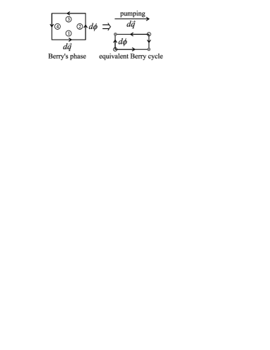
Figure 2: An infinitesimal cycle $C$ corresponding to Berry’s phase $\gamma_{m}(C)$ consists of four legs. The charge transfer $Q_{\rm p}$ for a fixed $\phi$ is identical to the Berry’s phase induced by traversing the legs in the shown directions. This path can not be followed continuously in the $(\vec{q},\phi)$-plane.

From here on the expression for the charging energy, Eq. (2), is examined in detail. This is done in order to rewrite the Hamiltonian in as simple a form as possible. In the homogeneous case the quadratic form is easily diagonalised and we find $N-1$ identical eigenvalues of $E_{\mathrm{C}}$ and one zero-energy mode in the direction of $\hat{v}_{0}:=(1,1,\ldots,1)/\sqrt{N}$. This demonstrates the uniqueness of the charging energy expression for each charge state and, consequently, the same zero-energy mode is observed in the inhomogeneous case, too.

In a proper representation of the $q$-space, the charging energy for homogeneous arrays can be expressed as $E_{\mathrm{C}}\|\tilde{q}\|_{2}^{2}$, where $\|\,\cdot\,\|_{2}$ is the usual Euclidean norm. Thus, the representatives of the tunnelling vectors $\{\vec{\delta}_{j}\}$, denoted by $\hat{q}_{j}$, are required. Above all, they must be normalised according to

$$\hat{q}_{j}\cdot\hat{q}_{k}=\delta_{jk}-1/N.$$ (9)

In an orthonormal $(N-1)$-dimensional basis, where $\hat{e}_{j}\cdot\hat{e}_{k}=\delta_{jk}$ and $\vec{x}=(x_{1},x_{2},\ldots,x_{N-1})$, the representatives define variables $\{\tilde{q}_{j}\}$ according to

$$\tilde{q}_{j}(\vec{x}):=\sum_{k=1}^{N-1}(e_{k}\cdot q_{j})x_{k}.$$ (10)

The normalisation condition (9) yields relations

$$\sum_{j=1}^{N}\tilde{q}_{j}=0\quad\mathrm{and}\quad\sum_{j=1}^{N}\tilde{q}_{j}^{2}=\sum_{j=1}^{N-1}x_{j}^{2}=\|\vec{x}\|^{2}$$ (11)

which are valid for all values of $\vec{x}$.

Suitable representatives for cases $N=3$ and $N=4$ are easy to find and their visualisation is obvious. When $N=3$, we select

$$\hat{q}_{1} = (\sqrt{2/3},0),\ \ \hat{q}_{2}=(-1/\sqrt{6},1/\sqrt{2}),$$ (12)

$$\hat{q}_{3} = (-1/\sqrt{6},-1/\sqrt{2}),$$ (13)

which describes three directions separated by identical $120^{\circ}$ angles. The resulting transformation of coordinates and the so-called honeycomb structure is shown in Fig. 3. The gate charges $q_{1}$ and $q_{2}$ determine the origin of the induced, rectangular coordinate system $(x_{1},x_{2})$.

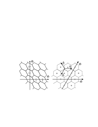
Figure 3: On the left-hand-side, the so-called honey comb structure induced by the charge state lattice ($N=3$). The regular lattice determined by the representatives $\hat{q}_{1}$, $\hat{q}_{2}$, and $\hat{q}_{3}$ is shown on the right-hand side. The origin of a new rectangular coordinate system $(x_{1},x_{2})$ is set by the gate charges $\vec{q}=(q_{1},q_{2})$. The charging energy for a charge state (gray circle) then reads $E_{\mathrm{C}}(x_{1}^{2}+x_{2}^{2})$, where the nearest-neighbour distance has been scaled to $\sqrt{2/3}$.

For $N=4$, symmetric representatives are given by the well-known body centered cubic lattice (BCC) of solid state physics, explicitly

$$\hat{q}_{1} = (1,1,-1)/2,\ \ \hat{q}_{2}=(1,-1,1)/2,$$ (14)

$$\hat{q}_{3} = (-1,1,1)/2,\ \ \hat{q}_{4}=(-1,-1,-1)/2.$$ (15)

These representatives are convenient when studying the case $N=4$, but a more general method for obtaining representaves is required. By augmenting the existing representatives for $N$ we can always obtain the set for $N+1$. The additional representative is set to lie along the new (first) coordinate axis with the correct length $\sqrt{N/(N+1)}$. The normalisation condition (9) is satisfied if all other representatives are retained as they were with an identical first component of $-1/\sqrt{N(N+1)}$.

Applying this method inductively, starting from trivial case of $N=1$, yields the general representives for any $N$. Let the length of the array be $N$ and denote the $j^{\mathrm{th}}$ representive and its $k^{\mathrm{th}}$ component by $\hat{q}^{N}_{j}$ and $q^{N}_{j(k)}$, respectively. The $N-1$ components are obtained from three simple rules:

$$(i) q^{N}_{j(j)}=\sqrt{(N-j)/(N+1-j)}$$ (16)

$$(ii) q^{N}_{j(k>j)}=0$$ (17)

$$(iii) q^{N}_{j(k<j)}=-1/\sqrt{(N-j)(N+1-j)}$$ (18)

The above transformation simplifies and symmetrices the tunnelling-charging Hamiltonian for arrays of any length. Inhomogeneous arrays can also be considered once the tools have been developed.

III Mathieu equation and discrete harmonic oscillator

The canonical form of the Mathieu equation readsAbramowitz and Stegun (1972)

$$\frac{d^{2}y}{dv^{2}}+(a-2q\cos(2v))y=0,$$ (19)

where $y(v)$ is the solution, $q$ is a parameter and $a$ is known as the characteristic value or eigenvalue.

The Hamiltonian of a SSET for a fixed phase difference $\phi$ in the charge state representation can be mapped onto a one dimensional discrete harmonic oscillator (DHO), see e.g. Ref. Tinkham, 1996; Aunola, 2002. Our chosen form includes a nearest-neighbour coupling $-\varepsilon_{\mathrm{J}}/2$ and the potential $V(n)=(n-n_{0})^{2}$, where $n$ is an integer. The equation for the amplitude $a_{n}$ now reads

$$(n-n_{0})^{2}a_{n}-(\varepsilon_{\mathrm{J}}/2)(a_{n-1}+a_{n+1})=Ea_{n},$$ (20)

where $E$ is the eigenvalue we are looking for. In order to obtain the solution of the discrete equation, we assume that $a_{n}$ is a continuous function an replace other amplitudes by respective Taylor expansions. We denote the step size by $h$ (here $h=1$) which yields

$$a_{n-h}+a_{n+h}=\sum_{k=0}^{\infty}\frac{2h^{2k}}{(2k)!}\frac{d^{2k}a_{n}}{dn^{2k}},$$ (21)

a differential equation for $a_{n}$.

We now transform into conjugate variables of the island charge, i.e. $n-n_{0}\rightarrow-id/d\theta$ and $id/dn\rightarrow\theta$. Collecting the terms, we find

$$\frac{d^{2}a(\theta)}{d\theta^{2}}+\left[E+(\varepsilon_{\mathrm{J}}/2)\cos(\theta)\right]a(\theta)=0,$$ (22)

which is identical to the Mathieu equation with $a=4E$ and $q=2\varepsilon_{\mathrm{J}}$ once we choose $\tilde{\theta}=(\theta+\pi)/2$.

In the limit $q\rightarrow\infty$, the ground state energy can be read from Eq. 20.2.30 of Ref. Abramowitz and Stegun, 1972 with the result

$$E_{0}^{\mathrm{DHO}}\hskip-2.0pt=\hskip-1.0pt-\varepsilon_{\mathrm{J}}\hskip-1.0pt+\hskip-1.0pt\frac{\sqrt{\varepsilon_{\mathrm{J}}}}{\sqrt{2}}\hskip-1.0pt-\hskip-1.0pt\frac{1}{16}\hskip-1.0pt-\hskip-1.0pt\frac{\sqrt{2/\varepsilon_{\mathrm{J}}}}{256}\hskip-1.0pt-\hskip-1.0pt\frac{3/\varepsilon_{\mathrm{J}}}{2048}\hskip-1.0pt+\hskip-1.0pt\mathcal{O}(\varepsilon_{\mathrm{J}}^{-3/2}),$$ (23)

confirmed by numerical diagonalisation, too. Returning to the charge state representation, we divide the eigenvalue problem by $\varepsilon_{\mathrm{J}}$ and define the oscillator frequency $\omega:=\sqrt{2/\varepsilon_{\mathrm{J}}}$ and scaled energy $\tilde{E}:=E/\varepsilon_{\mathrm{J}}+1$. The lowest order approximation becomes

$$-a^{\prime\prime}/2+\mbox{$\frac{1}{2}$}\omega^{2}(n-n_{0})^{2}a=\tilde{E},$$ (24)

which is analytically solvable with $\tilde{E}=\omega/2$ and $a(n)\propto\exp(-\omega(n-n_{0})^{2}/2)$. From here on, $n_{0}$ is omitted from the expression $(n-n_{0})$ for brevity.

The discretisation naturally affects the wave function and as well as the eigenenergy (23). The lowest order approximation $\psi_{1}$ for the discrete wave function $\psi_{d}$ is naturally a Gaussian wave function. The optimal, but unnormalised, wave function is given by

$$\psi_{1}(n)\propto\exp\left(-\frac{\omega n^{2}/2}{1-\omega/8}\right).$$ (25)

$$\psi_{1}^{\mathrm{ex}}(n)\propto n\exp\left(-\frac{\omega n^{2}/2}{1-27\omega/16}\right).$$ (26)

More accurate a wave function reads

$$\psi_{2}(n)\propto\exp\left(-\frac{\omega n^{2}(1-\omega^{2}n^{2}/48)/2}{1-3\omega/16}\right),$$ (27)

$$\psi_{2}^{\mathrm{ex}}(n)\propto\left(n-\frac{\omega^{2}n^{3}}{24}\right)\exp\left(-\frac{\omega(n^{2}-\omega^{2}n^{4}/48)/2}{1-147\omega/640}\right),$$ (28)

where a cutoff $(1-\omega^{2}n^{2}/48)\rightarrow 1$ must be applied for large enough values of $n$, when the deviation becomes greater than $20$–$30$ %. These wave functions have been compared against the result of numerical diagonalisation, $\psi_{d}$, by taking the norm of the difference, in short $\|\psi_{d}-\psi_{j}\|$, which yields approximately

$$\|\psi_{d}-\psi_{1}\| \approx 0.018/\sqrt{\varepsilon_{\mathrm{J}}},$$ (29)

$$\|\psi_{d}-\psi_{2}\| \approx 0.009/\varepsilon_{\mathrm{J}}.$$ (30)

Because both trial wave functions converge towards the actual eigenstate of the system, approximate eigenenergies corresponding to $\psi_{1}$ and $\psi_{2}$ can be easily evaluated. Setting $n_{0}=0$ and examining the equation for coefficient $a_{0}$ gives

$$E_{\psi_{j}}\sim-\varepsilon_{\mathrm{J}}(a_{1}/a_{0}),$$ (31)

where $\varepsilon_{\mathrm{J}}\rightarrow\infty$. Expanding the terms in powers of $\omega=\sqrt{2/\varepsilon_{\mathrm{J}}}$ gives the desired result. We find that $E_{\psi_{1}}$ first deviates from the constant order in which the term is $-1/8$ instead of the correct $-1/16$. As expected $E_{\psi_{2}}$ is much better, and even the term $-\sqrt{2/\varepsilon_{\mathrm{J}}}/256$ is correctly reproduced.

The significance of the corrections in $\psi_{2}(n)$ with respect to the continuous solutions is relatively clear. The denominator $1-3\omega/16$ cancels $3/4$ of the of the leading second order term $-(\omega/2)^{2}/2$ and gives the correct eigenenergy in the constant order. On the other hand, the term proportional to $n^{4}$ is related to the truncated differential operator

$$\frac{d^{2}}{dn^{2}}+\frac{1}{12}\frac{d^{4}}{dn^{4}}.$$ (32)

The coefficient $-\omega^{2}/48$ can be divided in two parts, namely $1/12$ and $-\omega^{2}/4$ which seems reasonable as the latter scales correctly as function of $\omega$, while the former changes if the step length $h$ is altered.

This approach is rather similar to that of Skeel and HardySkeel and Hardy (2001) although they consider time-dependent problems instead of eigenvalue problems. Systems of differential equations are replaced by modified equations which try to compensate for the discretisation error. The present potential is harmonic and in the conjugate representation truncated potentials are anharmonic in nature. Anharmonic oscillators have been studied, and exact eigenvalues have been obtained.Mei$\beta$ner and Steinborn (1999); Meurice (2002) Unfortunately, the sign of our leading correction is negative, so these works are not applicable here.

If there are two orthogonal and independent directions, the wave function factorises and the one-dimensional result can be generalised. Nevertheless, we make the following assumption which is to be justified later. Let our Hamiltonian be defined on a regular, discrete lattice of the coordinates $\vec{x}$ and the potential be isotropic and harmonic, i.e. $V(\vec{x})=\omega^{2}\|\vec{x}\|^{2}/2$. Interactions between (neigbouring) lattice sites are expanded in terms of partial derivates up the fourth order in a similar manner to Eq. (21). We postulate an analytical trial solution if the second order operator is the Laplacian and the modified PDE eigenvalue problem has the form

$$-\mbox{$\frac{1}{2}$}\left(\nabla^{2}+D_{4}/12\right)\psi+\mbox{$\frac{1}{2}$}\omega^{2}\|\vec{x}\|^{2}\psi=\tilde{E}\psi,$$ (33)

where $D_{4}$ is a fourth order partial differential operator. We define corresponding ’conjugate variable’ $\tilde{D}_{4}$ by replacing each partial derivative with respect to $x_{j}$ by $x_{j}$ itself. For example, if $D_{4}=(\nabla^{2})^{2}$, i.e. the square of the Laplacian, the conjugate variable is the fourth power of the norm, explicitly, $\tilde{D}_{4}=(\|\vec{x}\|^{2})^{2}=\|\vec{x}\|^{4}$. Our unnormalised trial wave function is given by

$$\psi_{2}(\vec{x})\propto\exp\left(\frac{-(\omega/2)(\|\vec{x}\|^{2}-\omega^{2}\tilde{D}_{4}/48)}{1-\alpha\omega}\right),$$ (34)

where $\alpha$ is chosen so that cancellation of the constant order term in energy is exactly $3/4$, just as the factor $3/16$ in Eq. (27). The conjugate variable $\tilde{D}_{4}$ gives the correct functional form, although a cutoff for too large values as compared to $\|\vec{x}\|^{2}$ must be naturally applied. Hopefully, the asymptotic convergence of the norm $\|\psi_{d}-\psi_{2}\|$ is better than $1/\sqrt{\varepsilon_{\mathrm{J}}}$. The general asymptotical solution for the discretised harmonic oscillator has geen recently given in Ref. Aunola, 2003a.

IV Strong Josephson coupling and homogeneous arrays at $\phi=0$

When the Josephson energy $E_{\mathrm{J}}$ is large as compared to charging energy $E_{\mathrm{C}}$ it seems preferable to express the Hamiltonian in terms of the phase differences $\phi_{j}$. We choose to remain in the charge state representation for two reasons. First, the charging Hamiltonian is difficult to evaluate in the independent phase representation. Additionally, the model Hamiltonian is already diagonal with respect to the total phase difference $\phi$. The model Hamiltonian can be approximately diagonalised and interactions between states with different values of $\phi$ should be included later.

The Hamiltonian equation is explicitly written in units of $E_{\mathrm{C}}$, and more specifically, each equation (row) of the eigenvalue problem is examined separately. Each charge state $\vec{n}$ is labeled according its position in the orthonormal coordinates $\vec{x}=(x_{1},\ldots,x_{N-1})$. In units of $E_{\mathrm{C}}$, the equation for the coefficient $a_{\vec{x}}$ reads

$$\|\vec{x}\|^{2}a_{\vec{x}}-\frac{\varepsilon_{\mathrm{J}}}{2}\sum_{j=1}^{N}(e^{-i\phi/N}a_{\vec{x}+\hat{q}_{j}}+e^{i\phi/N}a_{\vec{x}-\hat{q}_{j}})=Ea_{\vec{x}}.$$ (35)

Now, consider the case $\phi=0$ and large values of $\varepsilon_{\mathrm{J}}$ in detail. Writing the eigenvalue as $\tilde{E}:=N+E/\varepsilon_{\mathrm{J}}$ transforms the eigenvalue problem into

$$-\frac{1}{2}\sum_{j=1}^{N}(a_{\vec{x}-\hat{q}_{j}}\hskip-2.0pt-2a_{\vec{x}}\hskip-2.0pt+\hskip-2.0pta_{\vec{x}+\hat{q}_{j}})\hskip-2.0pt+\hskip-2.0pt\mbox{$\frac{1}{2}$}\omega^{2}\|\vec{x}\|^{2}a_{\vec{x}}=\tilde{E}a_{\vec{x}},$$ (36)

Using the procedure explained in the previous section, we can find the corresponding modified PDE. The truncation means that each term $(a_{\vec{x}-\hat{q}_{j}}-2a_{\vec{x}}+a_{\vec{x}+\hat{q}_{j}})$ corresponds to a second order derivative and a fourth order derivative. The sum of the second order derivatives yields the Laplacian operator $\nabla^{2}$ due to the second part of Eq. (11), and the form of the modified equation matches Eq. (33). Next, we must evaluate the form of $\tilde{D}_{4}$, find correct value of $\alpha$, and compare the resulting wave function and eigenenergie against numerically obtained results.

The simpler, optimal Gaussian wave function reads

$$\psi_{1}(\vec{x})\propto\exp\left(-\frac{\omega\|\vec{x}\|^{2}/2}{1-(N-1)\omega/(8N)}\right),$$ (37)

where the modification of $(N-1)/N$ in the denominator arises from the fact that $\|\hat{q}_{j}\|^{2}=(N-1)/N$. The optimality as well as the expected rate of convergence, i.e. $1/\sqrt{\varepsilon_{\mathrm{J}}}$, has been confirmed up to $N=10$.

In case $N=3$ we find that

$$D_{4}^{(N=3)}=(\nabla^{2})^{2}/2$$ (38)

and hence $\tilde{D}_{4}^{(N=3)}=\|\vec{x}\|^{4}/2$. Because $\|\hat{q}_{j}\|^{2}=2/3$, the improved wave function for $N=3$ reads

$$\psi_{2}^{(N=3)}\propto\exp\left(-\frac{(\omega\|x\|^{2}/2)(1-\omega^{2}\|x\|^{2}/96)}{1-\omega/8}\right).$$ (39)

This proves to be quite accurate as the norm of the error vanishes according to $\|\psi_{d}-\psi_{2}^{(N=3)}\|\approx 0.0045/\varepsilon_{\mathrm{J}}$. As arrays become longer, pure radial (energy) dependence is not enough, since the operators $D_{4}$ become more complicated. For the BCC representatives ($N=4$) the differential operator is given by

$$D_{4}:=\frac{3}{4}\left(\sum_{j=1}^{3}\frac{\partial^{2}}{\partial x_{j}^{2}}\right)^{2}-\frac{1}{2}\sum_{j=1}^{3}\frac{\partial^{4}}{\partial x_{j}^{4}},$$ (40)

corresponding to a wave function $\psi_{2}^{(4)}$ proprotional to

$$\exp\hskip-1.0pt\left(\hskip-1.0pt-\frac{(\omega/2)\left[\|x\|^{2}\hskip-1.0pt-\hskip-1.0pt\omega^{2}\left(\frac{\|x\|^{4}}{64}\hskip-1.0pt-\hskip-1.0pt\sum_{j=1}^{3}\frac{x_{j}^{4}}{96}\right)\right]}{1-9\omega/64}\right)\hskip-1.0pt.$$ (41)

Because $\langle x_{j}^{4}\rangle=\langle\|\vec{x}\|^{4}\rangle/5$, this also explains why the best energy dependent fit occurs at $3\omega\|\vec{x}\|^{4}/320$.

For longer arrays the expression for the fourth order differential operator becomes quite complicated and less informative. Fortunately, the value of the conjugate variable $\tilde{D}_{4}^{(N)}$ can be easily obtained for any point $\vec{x}$. The simple expression is based on inner product of the $\vec{x}$-space and the representatives $\hat{q}_{j}$, in short

$$\tilde{D}_{4}^{(N)}(\vec{x})=\sum_{j=1}^{N}(\hat{q}_{j}\cdot\vec{x})^{4}.$$ (42)

The differential operator $D_{N}$ can be read from the above expression by retaining the components of $\vec{x}$ in symbolic form and transforming each coordinate its corresponding partial derivative. The correct cancellation requirement implies that the general form of $\alpha$ is given by $\alpha=3(N-1)/16N$.

Thus, the general trial wave function $\psi_{2}^{(N)}$ becomes

$$\psi_{2}^{(N)}(\vec{x})=A\exp\left(-\frac{(\omega/2)(\|x\|^{2}-\omega^{2}\tilde{D}_{4}^{(N)}(\vec{x})/48)}{1-3(N-1)\omega/(16N)}\right),$$ (43)

where $A$ is a normalisation factor and $\tilde{D}_{N}(\vec{x})$ given in Eq. (42) is evaluated for all charge states in the used basis. A suitable cutoff with respect to $\omega^{2}\tilde{D}_{N}(\vec{x})/(48\|x\|^{2})$, e.g. between $0.2$ and $0.3$, is naturally important. The wave function is independent of the representives $\{\hat{q}_{j}\}$, but those given in Eq. (18) are probably the most convenient. The rate of convergence of the norm $\|\psi_{d}-\psi_{2}^{(N)}\|$ has been confirmed as $1/\varepsilon_{\mathrm{J}}$ up to $N=7$. Tentatively, the same applies for $N=10$, although diagonalisation was limited below $\varepsilon_{\mathrm{J}}\approx 20$.

The ground state energy is virtually independent of the gate charges $\vec{q}$ when $\varepsilon_{\mathrm{J}}$ is large enough. Thus $E_{0}^{(N)}$ can be approximately obtained as in the one-dimensional case, see Eq. (31). All $2N$ neighbouring amplitudes are identical which now gives

$$E_{0}^{(N)}\approx-N\varepsilon_{\mathrm{J}}\exp\left[-\frac{(\omega/2)\left(\frac{N-1}{N}-\frac{\omega^{2}(N-1)^{2}}{48N^{2}}\right)}{1-3(N-1)\omega/(16N)}\right].$$ (44)

Expansion in powers of $\omega$ yields the asymptotic expansion

$$E_{0}^{(N)}\hskip-1.0pt\sim\hskip-1.0pt-N\varepsilon_{\mathrm{J}}\hskip-0.5pt+\hskip-0.5pt(N-1)\sqrt{\frac{\varepsilon_{\mathrm{J}}}{2}}\hskip-0.5pt-\hskip-0.5pt\frac{(N-1)^{2}}{16N}\hskip-1.0pt+\hskip 0.0pt\mathcal{O}\hskip-2.0pt\left(\varepsilon_{\mathrm{J}}^{-1/2}\right)\hskip-1.0pt,$$ (45)

verified by direct comparison against the numerically obtained eigenvalue for cases which allow diagonalisation. No analytical expression for the term proportional to $1/\sqrt{\varepsilon_{\mathrm{J}}}$ have been found, but it is not correctly reproduced, either. Direct calculation, using a method proposed in Refs. Aunola, 2003a and Aunola, 2003b, validates the above ansatz and corresponding asymptotical eigenenergy for $N\leq 42$, though.tek We now proceed to the the case when $\phi$ is no longer zero.

V Effects due to non-zero phase difference

For non-zero values of the phase difference $\phi$ the wave function becomes complex valued because the nearest neighbour coupling contains a term $e^{\pm i\phi/N}$. When $\phi$ is sufficiently small the phase does not vary significantly between nearest neighbours and as the first approximation the phase can be neglected in the corresponding equations. We then consider the absolute value of the amplitudes and observe that the differential operator is simply multiplied by a factor $\cos(\phi/N)$.

Consequently, the approximate eigenvalue problem to the original one, except that $\omega$ is replaced by $\tilde{\omega}=\omega/\sqrt{\cos(\phi/N)}$. The ground state energy can be obtained from Eq. (45) with $\varepsilon_{\mathrm{J}}\rightarrow\varepsilon_{\mathrm{J}}\cos(\phi/N)$. The accuracy of this expression is rather good, even for large values of $\phi$ if $\varepsilon_{\mathrm{J}}$ is sufficiently large. The convergence in terms of the absolute values of the amplitudes is satisfactory, too. Convergence in terms of trial wave function $|\tilde{\psi}_{1}|$ goes clearly as $1/\sqrt{\varepsilon_{\mathrm{J}}}$ and that of $|\tilde{\psi}_{2}|$ goes nearly as $1/\varepsilon_{\mathrm{J}}$, weakening as $\phi$ increases.

In order to consider the complex wave function explicitly, the approximate differential operator induced by $\phi$ must be constructed. The first order differential operator is always cancelled on behalf of the first property in Eq. (11). The common prefactor of the third order terms, relative to the Laplace operator, is here $-i\sin(\phi/N)/3$. Because the conjugate coordinate $\tilde{D}_{4}^{(N)}$ was so successful in describing the homogeneous case, we define a third order conjugate coordinate which evaluates to

$$\tilde{D}_{3}^{(N)}(\vec{x})=\sum_{j=1}^{N}(\hat{q}_{j}\cdot\vec{x})^{3}.$$ (46)

The first guess for the phase of the trial wave function is then given by

$$\frac{\psi_{2}(\vec{x})}{|\psi_{2}(\vec{x})|}\approx\exp\left(-\frac{(\tilde{\omega}/2)(-i\tilde{\omega}\tilde{D}_{N}^{(3)})/(6N)}{1-3(N-1)\tilde{\omega}/(16N)}\right),$$ (47)

where $\sin(\phi/N)$ has been approximated by $\phi/N$. Numerical diagonalisation clearly confirms the dependence on $\tilde{D}_{N}^{(3)}$, although a numerical correction factor $b_{\phi}$ of the order of $0.7$–$0.75$ for all $N$ has to be added. Additionally, but expectedly, the phase dependence is slowly dampened for larger values of $\|\vec{x}\|$. Yhe magnitude of these amplitudes rapidly decreases which makes the imaginary components even smaller. Thus, the leading component of the phase simplifies to

$$\exp(ib_{\phi}\sin(\phi/N)\tilde{\omega}^{2}D_{N}^{(3)}/12),$$ (48)

where $b_{\phi}\approx 0.7$. Finally, we turn in the direction of inhomogeneous array.

VI Inhomogeneous arrays and renormalisability

Our main aim is to obtain a wave function similar to $\psi_{1}$ in the inhomogeneous case at $\phi=0$ and, subsequently, improve this wave function. Effects due to non-zero $\phi$ are treatable in principle, but the expression become rather messy and accuracy is not that good. It suffices to say that the behaviour of the eigenenergy corresponds to the effective coupling strength $\varepsilon_{\mathrm{J}}\cos(\phi/N)$.

In the inhomogeneous case the charging energy reads

$$E_{\mathrm{C}}\left[\sum_{j=1}^{N}\frac{v_{j}^{2}}{c_{j}}-\frac{1}{N}\left(\sum_{j=1}^{N}\frac{v_{j}}{c_{j}}\right)^{2}\right].$$ (49)

The biasing to zero voltage implies that $\sum_{j=1}^{N}(v_{j}/c_{j})=0$, although the above expression is invariant under transformation $v_{j}\rightarrow v_{j}+y$. As each coupling is multiplied by $c_{j}$, the second order approximation for the Hamiltonian becomes

$$-\frac{1}{2}\sum_{j=1}^{N}\frac{c_{j}}{\beta^{2}}\frac{\partial^{2}}{\partial(\beta\hat{q}_{j})^{2}}+\frac{\omega^{2}\hat{q}_{j}^{2}}{2c_{j}},$$ (50)

where $\beta=\sqrt{N/(N-1)}$. For sufficiently small values of $\omega$ and reasonably homogeneous arrays the condition $\sum_{j=1}^{N}(v_{j}/c_{j})=0$ does not vary much between neighbouring points. In other words, the error between different lines of the eigenvalue equation is insignificant. Under those circumstances we renormalise the coordinates according to

$$v_{j}\rightarrow\tilde{v}_{j}=v_{j}/\sqrt{c_{j}},$$ (51)

which yields a Hamiltonian identical to the homogeneous case. In a similar manner, we write the the lowest order wave function as

$$\psi_{1}^{(\mathrm{inh})}(\vec{x})\propto\exp\left(-\frac{(\omega/2)\sum_{j=1}^{N}(v_{j}^{2}/c_{j})}{1-(N-1)\omega/8}\right).$$ (52)

where the summation gives simply the charging energy corresponding to $\vec{x}$. This is the best Gaussian wave function in the renormalised coordinates $\tilde{v}_{j}$ and the rate of convergence of the error the expected $1/\sqrt{\varepsilon_{\mathrm{J}}}$.

The Hamiltonian of an inhomogeneous Cooper pair pump is thus renormalisable and the leading terms in the eigenenergy are

$$E_{0,\mathrm{inh}}^{(N)}\approx-\varepsilon_{\mathrm{J}}\sum_{j=1}^{N}c_{j}+(N-1)\sqrt{\frac{\varepsilon_{\mathrm{J}}}{2}}+\mathcal{O}(1).$$ (53)

The constant term can also be evaluated if we assume a cancellation of $3/4$ in this term which is correct for homogeneous arrays. We simplify the expression

$$-\frac{1}{16}\sum_{j=1}^{N}\frac{1}{c_{j}}\left[1-1/(Nc_{j})\right]^{2}$$ (54)

by denoting $b_{j}:=(1/c_{j}-1)$ and collecting the terms. Not so unexpectedly, and as in Ref. Aunola et al., 2000, the deviation from the homogeneous value is dominantly proportional to the square of the inhomogeneity index $X_{\mathrm{inh}}$. The result,

$$\frac{-(N-1)^{2}-(2N-3)X_{\mathrm{inh}}^{2}+\sum_{j=1}^{N}(b_{j}^{3}/N)}{16N},$$ (55)

has been confirmed up to $N=6$ if only a single capacitance deviates from the others. In case $N=3$ this expression has been tested more rigorously and further corrections do vanish as $1/\sqrt{\varepsilon_{\mathrm{J}}}$.

In order to improve the results, more elaborate transformations are required. The most viable transformation is based on diagonalising the charging energy and transforming the representation space ($\vec{x}$-space) in such a manner that the charging energy is proportional to the square of the new norm. New representatives $\hat{q}^{\prime}_{j}$ are obtained and the differential operators in the second and fourth order can be obtained. For some special cases, the second order differential operator is of the Laplace type, i.e. the conjugate coordinate is given by

$$\tilde{D}^{\prime}_{2}(\vec{x}^{\prime})=\sum_{j=1}^{N}c_{j}(\hat{q}^{\prime}_{j}\cdot\vec{x}^{\prime})^{2}=\|\vec{x}^{\prime}\|^{2}.$$ (56)

In those cases the fourth order coordinate

$$\tilde{D}^{\prime}_{4}(\vec{x}^{\prime})=\sum_{j=1}^{N}c_{j}(\hat{q}^{\prime}_{j}\cdot\vec{x}^{\prime})^{4}$$ (57)

yields a trial wave function which can be compared against the numerically obtained wave function. In most cases, the Laplacian operator is slightly distorted, but for small inhomogeneities this can be neglected as the first approximation. In both cases the results are not as good as in the homogeneous case, but the improvement with respect to Eq. (52) is significant. Due to dimensional limitations the comparisons between wave functions have been performed when $N=3$.

As shown by the cancellation in the eigenenergy, no isotropic value of $\alpha$ such as $3(N-1)/16N$ in Eq. (43) is can be used. Rescaling of the coordinates changes the optimal value of $\alpha$ in different directions, and some further improvement may be obtained by using a non-isotropic $\alpha(\vec{x})$ in the calculations. Minor improvements can be obtained by fiddling with the coefficients of the coordinates, too. We conclude this section by stating that significant improvement of the wave function has been obtained, but so far no analytical expressions have been able to reach asymptotical convergence better than $1/\sqrt{\varepsilon_{\mathrm{J}}}$.

VII Conclusions

We have developed a method for obtaining an (approximate) analytical solution for Laplace type eigenvalue equations with a harmonic potential and discreteness induced higher order corrections. In the one-dimensional case corresponding to the Mathieu equation the results were convincing and thus we applied the proposed method on the tunnelling-charging Hamiltonian of an ideally biased Cooper pair pump.

We have obtained reliable analytical expressions for the ground state wave function and energy for homogeneous arrays of arbitrary length. Furthermore, effects due to nonvanishing phase difference were relatively well described and the Hamiltonian of an inhomogeneous pump was shown to be renormalisable. Again, reliable eigenenergies and reasonable eigenfunctions were obtained. Further improvements in the inhomogeneous case have been proposed and partially carried out, too.