[

Electric Field Induced Kondo Tunneling Through Double Quantum Dot

Abstract

It is shown that the resonance Kondo tunneling through a double quantum dot (DQD) with even occupation and singlet ground state may arise at a strong bias, which compensates the energy of singlet/triplet excitation. Using the renormalization group technique we derive scaling equations and calculate the differential conductance as a function of an auxiliary dc-bias for parallel DQD.

PACS numbers: 72.10.-d, 72.10.Fk, 72.15.Qm, 05.10.Cc

]

Many fascinating collective effects, which exist in strongly correlated electron systems (metallic compounds containing transition and rare-earth elements) may be observed also in artificial nanosize devices (quantum wells, quantum dots, etc). Moreover, fabricated nanoobjects provide unique possibility to create such conditions for observation of many-particle phenomena, which by no means may be reached in ”natural” conditions. Kondo effect (KE) is one of such phenomena. It was found theoretically [1] and observed experimentally [2] that the charge-spin separation in low-energy excitation spectrum of quantum dots under strong Coulomb blockade manifests itself as a resonance Kondo-type tunneling through a dot with odd electron occupation ${\cal N}$ (one unpaired spin 1/2). This resonance tunneling through a quantum dot connecting two metallic reservoirs (leads) is an analog of resonance spin scattering in metals with magnetic impurities. A Kondo-type tunneling may be observed under conditions which do not exist in conventional metallic compounds. In particular, Kondo effect survives in essentially non-equilibrium state when the strong bias $eV\gg T_{K}$ is applied between the leads [3] ($T_{K}$ is the Kondo temperature which determines the energy scale of low-energy spin excitations in a quantum dot). The KE may be observed as a dynamical phenomenon in strong time dependent electric field [4], it may arise at finite frequency under light illumination [5]. Even the net zero spin of isolated quantum dot (even ${\cal N}$) is not the obstacle for the resonance Kondo tunneling. In this case it may be observed in specific types of double quantum dots (DQD) [6] or induced by strong magnetic field [7] whereas in conventional metals magnetic field only suppresses the Kondo scattering. The latter effect was also observed experimentally [8].

As was noticed in [6, 9], quantum dots with even ${\cal N}$ possess the dynamical symmetry $SO(4)$ of spin rotator in the Kondo tunneling regime, provided the low-energy part of its spectrum is formed by a singlet-triplet (ST) pair, and all other excitations are separated from the ST manifold by a gap noticeably exceeding the tunneling rate $\gamma$. A DQD with even ${\cal N}$ in a side-bound configuration where two wells are coupled by the tunneling $v$ and only one of them (say, $l$) is coupled to metallic leads $(L,R)$ is a simplest system satisfying this condition [6]. Such system was realized experimentally in Ref.[10].

In the present paper one more unusual property of DQDs with even ${\cal N}$ is revealed. It is shown that in the case when the ground state is singlet $|S\rangle$ and the ST gap $\delta\gg T_{K}$, a Kondo resonance channel arises under a strong bias $eV$ comparable with $\delta.$ The channel opens at $|eV-\delta|<T_{K}$, and the Kondo temperature is determined by the non-diagonal component $J_{ST}=\langle T|J|S\rangle$ of effective exchange induced by the electron tunneling through DQD (Fig. 1b).

a)                                    b)

FIG. 1.: (a) Double quantum dot in a side-bound configuration (b) co-tunneling processes in biased DQD responsible for the resonance Kondo tunneling.

The basic properties of symmetric DQD occupied by even number of electrons ${\cal N}=2n$ under strong Coulomb blockade in each well are manifested already in the simplest case $n=1$, which is considered below. Such DQD is an artificial analog of a hydrogen molecule ${\rm H_{2}}$. If the inter-well Coulomb blockade $Q$ is strong enough, one has ${\cal N}=n_{l}+n_{r},$ $n_{l}=n_{r}=1,$ the lowest states of DQD are singlet and triplet and the next levels are separated from ST pair by a charge transfer gap $\sim Q$. We assume that both wells are neutral at $n_{l,r}=1$. Then the effective inter-well exchange responsible for the singlet-triplet splitting arises because of tunneling $V$ between two wells, $J=v^{2}/Q=\delta$. It is convenient to write the effective spin Hamiltonian of isolated DQD in the form

$$H_{d}=E_{S}|S\rangle\langle S|+\sum_{\eta}E_{T}|T\eta\rangle\langle T\eta|\equiv\sum_{\Lambda=S,T\eta}E_{\Lambda}X^{\Lambda\Lambda}$$ (1)

where $X^{\Lambda\Lambda^{\prime}}=|\Lambda\rangle\langle\Lambda^{\prime}|$ is a Hubbard configuration change operator (see, e,g, [11]), $E_{T}=E_{S}+\delta$, $\eta=\pm,0$ are three projections of $S=1$ vector. Two other terms completing the Anderson Hamiltonian, which describes the system shown in Fig.1a, are

$$H_{b}+H_{t}=$$

$$\sum_{k\alpha\sigma}\epsilon_{k\alpha}c^{\dagger}_{k\alpha\sigma}c_{k\alpha\sigma}+W\sum_{\Lambda\lambda}\sum_{k\sigma}\left(c_{kl\sigma}^{\dagger}X^{\lambda\Lambda}+H.c.\right).$$ (2)

The first term describes metallic electrons in the leads and the second one stands for tunneling between the leads and the DQD. Here $\alpha=L,R$ marks electrons in the left and right lead, respectively, the bias $eV$ is applied to the left lead, so that the chemical potentials are $\mu_{FL}=\mu_{FR}+eV$,  $W$ is the tunneling amplitude for the well $l$, $|\lambda\rangle$ are one-electron states of DQD, which arises after escape of an electron with spin projection $\sigma$ from DQD in a state $|\Lambda\rangle$.

In case of strong Coulomb blockade $Q\gg\gamma$, the non-equilibrium repopulation of DQD is a weak effect and one may start with a second order perturbation calculation in tunneling amplitude known as the Schrieffer-Wolff (SW) transformation [11], where both leads are considered as independent subsystems. As is shown in Refs. [6, 9] the SW transformation being applied to a spin rotator results in the following effective spin Hamiltonian

$$H_{int}=\sum_{\alpha\alpha^{\prime}}[(J^{TT}_{\alpha\alpha^{\prime}}{\bf S}+J^{ST}_{\alpha\alpha^{\prime}}{\bf P})\cdot{\bf s}_{\alpha\alpha^{\prime}})+J^{SS}_{\alpha\alpha^{\prime}}X^{SS}n_{\alpha\alpha^{\prime}}]$$ (3)

Here ${\bf s}_{\alpha\alpha^{\prime}}$$=$$\sum_{kk^{\prime}}c^{\dagger}_{k\alpha\sigma}\hat{\tau}c_{k^{\prime}\alpha^{\prime}\sigma^{\prime}}$,  $n_{\alpha\alpha^{\prime}}$$=$$\sum_{kk^{\prime}}c^{\dagger}_{k\alpha\sigma}\hat{1}c_{k^{\prime}\alpha^{\prime}\sigma}$, $\hat{\tau}$,  $\hat{1}$ are the Pauli matrices and unity matrix respectively. The effective exchange constants are

$$J^{\Lambda\Lambda^{\prime}}_{\alpha\alpha^{\prime}}\approx\frac{W^{2}}{2}\left(\frac{1}{\epsilon_{F\alpha}-(E_{S}/2+\delta)}+\frac{1}{\epsilon_{F\alpha^{\prime}}-(E_{S}/2+\delta)}\right)$$

Two vectors ${\bf S}$ and ${\bf P}$ with spherical components

$$S^{+}=\sqrt{2}\left(X^{10}+X^{0-1}\right),~{}S^{-}=\sqrt{2}\left(X^{01}+X^{-10}\right),$$ (4)

$$S_{z}=X^{11}-X^{-1-1},\,\;\;\;P_{z}=-\left(X^{0S}+X^{S0}\right),$$ (5)

$$P^{+}=\sqrt{2}\left(X^{1S}-X^{S-1}\right),P^{-}=\sqrt{2}\left(X^{S1}-X^{-1S}\right).$$ (6)

obey the commutation relations of $o_{4}$ algebra

$\displaystyle[S_{j},S_{k}]=ie_{jkl}S_{l},~{}[P_{j},P_{k}]=ie_{jkl}S_{l},~{}[P_{j},S_{k}]=ie_{jkl}P_{l}$

($j,k,l$ are Cartesian coordinates, $e_{jkl}$ is a Levi-Chivita tensor). These vectors are orthogonal, ${\bf S\cdot P}=0,$ and the Casimir operator is ${\bf S}^{2}+{\bf P}^{2}=3.$ Thus, the singlet state is involved in spin scattering via the components of the vector ${\bf P}$.

We use $SU(2)$-like semi-fermionic representation for $S$ operators [12, 13]

$$S^{+}=\sqrt{2}(f_{0}^{\dagger}f_{-1}+f^{\dagger}_{1}f_{0}),\;\;\;S^{-}=\sqrt{2}(f^{\dagger}_{-1}f_{0}+f_{0}^{\dagger}f_{1}),$$

$$S_{z}=f^{\dagger}_{1}f_{1}-f^{\dagger}_{-1}f_{-1},$$ (7)

where $f^{\dagger}_{\pm}$ are creation operators for fermions with spin “up” and “down” respectively, whereas $f_{0}$ stands for spinless fermion [12, 13]. This representation can be generalized for $SO(4)$ group by introducing another spinless fermion $f_{s}$ to take into consideration the singlet state. As a result, the $P$-operators are given by the following equations:

$$P^{+}=\sqrt{2}(f^{\dagger}_{1}f_{s}-f_{s}^{\dagger}f_{-1}),\;\;\;P^{-}=\sqrt{2}(f_{s}^{\dagger}f_{1}-f^{\dagger}_{-1}f_{s}),$$

$$P^{z}=-(f_{0}^{\dagger}f_{s}+f_{s}^{\dagger}f_{0}).$$ (8)

The Casimir operator ${\bf S}^{2}+{\bf P}^{2}=3$ transforms to the local constraint $\sum_{\Lambda=\pm,0,s}f^{\dagger}_{\Lambda}f_{\Lambda}=1$.

The spin Hamiltonian is now given by

$$H_{int}=\sum_{kk^{\prime},\alpha\alpha^{\prime}=L,R}J^{S}_{\alpha\alpha^{\prime}}f_{s}^{\dagger}f_{s}c^{\dagger}_{k\alpha\sigma}c_{k^{\prime}\alpha^{\prime}\sigma}$$ (9)

$$+\sum_{kk^{\prime},\alpha\alpha^{\prime}\Lambda\Lambda^{\prime}}\left(J^{T}_{\alpha\alpha^{\prime}}\hat{S}^{d}_{\Lambda\Lambda^{\prime}}+J^{ST}_{\alpha\alpha^{\prime}}\hat{P}^{d}_{\Lambda\Lambda^{\prime}}\right)\tau^{d}_{\sigma\sigma^{\prime}}c^{\dagger}_{k\alpha\sigma}c_{k^{\prime}\alpha^{\prime}\sigma^{\prime}}f_{\Lambda}^{\dagger}f_{\Lambda^{\prime}}$$

where $\hat{S}^{d}$ and $\hat{P}^{d}$ ($d$$=$$x$,$y$,$z$) are $4\times 4$ matrices defined by relations (6) - (8) and $J^{S}=J^{SS}$, $J^{T}=J^{TT}$ and $J^{ST}$ are singlet, triplet and singlet-triplet coupling SW constants, respectively.

To develop the perturbative approach for $T>T_{K}$ we introduce the temperature Green’s functions (GF) for electrons in a dot, ${\cal G}_{\Lambda}(\tau)=-\langle T_{\tau}f_{\Lambda}(\tau)f^{\dagger}_{\Lambda}(0)\rangle,$ and GF of left (L) and right (R) electrons in the leads $G_{L,R}(k,\tau)=-\langle T_{\tau}c_{L,R\sigma}(k,\tau)c^{\dagger}_{L,R\sigma}(k,0)\rangle$. Performing a Fourier transformation in imaginary time for bare GF’s, we come to following expressions:

$$G^{0}_{k\alpha}(\epsilon_{n})=(i\epsilon_{n}-\epsilon_{k}+\mu_{L,R})^{-1},$$

$${\cal G}^{0}_{\eta}(\omega_{m})=(i\omega_{m}-E_{T})^{-1},\;\;\;\eta=-1,0,1$$

$${\cal G}^{0}_{s}(\epsilon_{n})=(i\epsilon_{n}-E_{S})^{-1},$$ (10)

with $\epsilon_{n}=2\pi T(n+1/2)$ and $\omega_{m}=2\pi T(m+1/3)$ [12, 13]. The first leading and next to leading parquet diagrams are shown on Fig.2.

In equilibrium state $eV=0$ the elastic Kondo tunneling arises only provided $T_{K}\gg\delta$ in accordance with the theory of two-impurity Kondo effect [9, 14]. Now we will show that in the opposite limit $T_{K}\ll\delta$ the elastic channel emerges at $eV\approx\delta$.

Corrections to the singlet vertex $\Gamma(\omega,0;\omega,eV)$ are calculated using an analytical continuation of GF’s to the real axis $\omega$ and taking into account the shift of the chemical potential in the left lead. In a weak coupling regime $T>T_{K}$ the leading non-Born contributions to the tunnel current are determined by the diagrams of Fig. 2 b-e.

FIG. 2.: Leading (b,d) and next to leading (c,e) parquet diagrams determining renormalization of $J^{S}(a)$. Solid lines denote electrons in the leads. Dashed lines stand for electrons in the dot.

The effective vertex shown in Fig. 2b is given by the following equation

$$\Gamma_{LR}^{(2b)}(\omega)=J_{LL}^{ST}J_{LR}^{TS}\sum_{\bf k}\frac{1-f(\epsilon_{kL}-eV)}{\omega-\epsilon_{kL}+\mu_{L}-\delta}$$ (11)

Changing the variable $\epsilon_{kL}$ for $\epsilon_{kL}-eV$ one finds that $\Gamma_{LR}^{(2b)}(\omega)\sim J_{LL}^{ST}J_{LR}^{TS}\nu\ln~{}(D/{\rm max}\{\omega,(eV-\delta),T\})$. Here $D\sim\varepsilon_{F}$ is a cutoff energy determining effective bandwidth, $\nu$ is a density of states on a Fermi level and $f(\varepsilon)$ is the Fermi function. Therefore, under condition $|eV-\delta|\ll\max[eV,\delta]$ this correction does not depend on $eV$ and becomes quasielastic.

Unlike the diagram Fig. 2b, its ”parquet counterpart” term Fig. 2c contains $eV+\delta$ in the argument of the Kondo logarithm:

$$\Gamma_{LR}^{(2c)}(\omega)=J_{LL}^{ST}J_{LR}^{TS}\sum_{\bf k}\frac{f(\epsilon_{kL}-eV)}{\omega-\epsilon_{kL}+\mu_{L}+\delta}$$ (12)

At $eV\sim\delta\gg T,\omega$ this contribution is estimated as $\Gamma_{LR}^{(2c)}(\omega)\sim J_{LL}^{ST}J_{LR}^{TS}\nu\ln~{}(D/(eV+\delta))\ll\Gamma_{LR}^{(2b)}(\omega)$.

Similar estimates for diagrams Fig.2d and 2e give

$$\Gamma_{LR}^{(2d)}(\omega)\sim J_{LL}^{ST}J_{LL}^{T}J_{LR}^{TS}\nu^{2}\ln^{2}~{}(D/{\rm max}\{\omega,(eV-\delta),T\})$$

$$\Gamma_{LR}^{(2e)}(\omega)\sim J_{LL}^{ST}J_{LL}^{T}J_{LR}^{TS}\nu^{2}\ln~{}(D/{\rm max}\{\omega,(eV-\delta),T\})\times$$

$$\times\ln~{}(D/{\rm max}\{\omega,eV,T\}.$$ (13)

Then $\Gamma_{LR}^{(2e)}(\omega)\ll\Gamma_{LR}^{(2d)}(\omega)$ at $eV\to\delta$.

Thus, the Kondo singularity is restored in strongly non-equilibrium conditions when the energy loss $\delta$ in a singlet-triplet excitation is compensated by the external voltage applied to the lead, but the leading sequence of most divergent diagrams degenerates in this case from a parquet to a ladder series.

Following the poor man’s scaling approach, we derive the system of coupled renormalization group (RG) equations for (9). The equations for LL co-tunneling are:

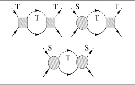
FIG. 3.: Irreducible diagrams contributing to RG equations. Hatched boxes and circles stand for triplet-triplet and singlet-triplet vertices respectively. Notations for lines are the same as in Fig.2

$$\frac{dJ^{T}_{LL}}{d\ln D}=-\nu(J_{LL}^{T})^{2},\;\;\;\frac{dJ^{ST}_{LL}}{d\ln D}=-\nu J_{LL}^{ST}J_{LL}^{T},$$ (14)

The scaling equations for $J_{LR}^{\Lambda}$ are as follows:

$$\frac{dJ^{T}_{LR}}{d\ln D}=-\nu J_{LL}^{T}J_{LR}^{T},\;\;\;\frac{dJ^{ST}_{LR}}{d\ln D}=-\nu J_{LL}^{ST}J_{LR}^{T},$$

$$\frac{dJ^{S}_{LR}}{d\ln D}=\frac{1}{2}\nu\left(J_{LL,+}^{ST}J_{LR,-}^{TS}+\frac{1}{2}J_{LL,z}^{ST}J_{LR,z}^{TS}\right).$$ (15)

One-loop diagrams corresponding to the poor man’s scaling procedure are shown in Fig. 3. To derive these equations we collected only terms $\sim(J^{T})^{n}\ln^{n+1}(D/T)$ neglecting contributions containing $\ln[D/(eV)]$. The analysis of RG equations beyond the one loop approximation will be published elsewhere.

The solution of the system (15) reads as follows:

$$J^{T}_{\alpha,\alpha^{\prime}}=\frac{J^{T}_{0}}{1-\nu J^{T}_{0}\ln(D/T)},\;\;\;J^{ST}_{\alpha,\alpha^{\prime}}=\frac{J^{ST}_{0}}{1-\nu J^{T}_{0}\ln(D/T)},$$

$$J^{S}_{LR}=J^{S}_{0}-\frac{3}{4}\nu(J^{ST}_{0})^{2}\frac{\ln(D/T)}{1-\nu J^{T}_{0}\ln(D/T)}.$$ (16)

Here $\alpha=L$, $\alpha^{\prime}=L,R$. The Kondo temperature is determined by triplet-triplet processes only. It is given by $T_{K}=D\exp[-1/(\nu J^{T}_{0})]$.

The differential conductance $G(eV,T)/G_{0}$ is the universal function of two parameters $T/T_{K}$ and $V/T_{K}$ (see Fig. 4), $G_{0}=e^{2}/\pi\hbar$:

$$G/G_{0}\sim\ln^{-2}\left(\max[(eV-\delta),T]/T_{K}\right)$$ (17)

Finite decoherence rate $\hbar/\tau_{d}$ effects discussed in [16] in a context of strongly-nonequilibrium transport through QD with $S=1/2$ do not arise in our case. According to the Non-Crossing Approximation (NCA) description, the origin of $\tau_{d}$ is inelastic spin relaxation of Kondo state. In the problem considered the ground state is $S=0$ singlet and the spin-relaxation is absent. A Kondo-channel arises only in virtual states of L-R co-tunneling. Repopulation effects at $eV>\delta$ should result in asymmetry of Kondo-peak [16], but this effect is beyond our quasi equilibrium approach.

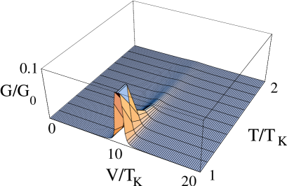
FIG. 4.: The Kondo conductance as a function of dc-bias $eV/T_{K}$ and $T/T_{K}$. The singlet-triplet splitting $\delta/T_{K}=10$.

Thus, we have shown that the tunneling through singlet DQDs with $\delta\gg T_{K}$ exhibits a peak in differential conductance at $eV\approx\delta$ instead of the usual zero bias Kondo anomaly (see Fig. 4) which arises in the opposite limit, $\delta<T_{K}$. Therefore, in this case the Kondo effect in DQD is induced by a strong external bias. The scaling equations (15), (16) can also be derived in Schwinger-Keldysh formalism (see [13] and also [16]) by applying the “poor man’s scaling” approach directly to the dot conductance [4]. The detailed analysis of the model (9) in a real-time formalism will be presented elsewhere.

We discuss yet another possible experimental realization of resonance Kondo tunneling driven by external electric field. Applying the alternate field $V=V_{ac}\cos(\omega t)$ to the parallel DQD, one takes into consideration two effects, namely (i) enhancement of Kondo conductance by tuning the amplitude of ac-voltage to satisfy the condition $|eV_{ac}-\delta|\ll T_{K}$ and (ii) spin decoherence effects due to finite decoherence rate [4]. One can expect that if the decoherence rate $\hbar/\tau\gg T_{K},$

$$G_{peak}/G_{0}\sim\ln^{-2}\left(\hbar/\tau T_{K}\right)$$ (18)

whereas in the opposite limit $\hbar/\tau\ll T_{K}$,

$$G_{peak}=\overline{G(V_{ac}\cos[\omega t])}$$ (19)

is averaged over a period of variation of ac bias. In this case the estimate (17) is also valid.

In conclusion, we have provided the first example of Kondo effect, which exists only in non-equilibrium conditions. It is driven by external electric field in tunneling through a quantum dot with even number of electrons, when the low-lying states are those of spin rotator. This is not too exotic situation because as a rule, a singlet ground state implies a triplet excitation. If the ST pair is separated by a gap from other excitons, then tuning the dc-bias in such a way that applied voltage compensates the energy of triplet excitation, one reaches the regime of Kondo peak in conductance. This theoretically predicted effect can be observed in dc- and ac-biased double quantum dots in parallel geometry.

This work is partially supported (MK) by the European Commission under LF project: Access to the Weizmann Institute Submicron Center (contract number: HPRI-CT-1999-00069). The authors are grateful to Y. Avishai, A. Finkel’stein, Y. Gefen, H. Kroha, A. Rosch and M.Heiblum for numerous useful discussions. The financial support of the Deutsche Forschungsgemeinschaft (SFB 410) is gratefully acknowledged. The work of KK is supported by ISF grant.

REFERENCES

[1] L.I.Glazman and M.E.Raikh, JETP Lett. 47,
452, (1988); T.K.Ng and P.A.Lee, Phys.Rev.Lett., 61, 1768 (1988).
[2] D. Goldhaber-Gordon et.al., Phys.Rev.Lett. 81,
5225 (1998); S.M. Cronenwett et al., Science, 281, 540 (1998);
F. Simmel et al., Phys. Rev. Lett. 83, 804 (1999).
[3] Y. Meir et al, Phys.Rev.Lett.
68, 2512 (1992), Phys.Rev. B49, 11040 (1994);
T.K. Ng, Phys. Rev. Lett. 76, 487 (1996);
M.H. Hettler et al, Phys. Rev. B58, 5649 (1998);
[4] Y. Goldin and Y. Avishai, Phys. Rev. Lett. 81, 5394
(1998), Phys. Rev. B61, 16750
(2000); A. Kaminski et al, Phys. Rev. B62,
8154 (2000); R. Lopez et al, Phys. Rev. B 64, 075319 (2001).
[5] K. Kikoin and Y. Avishai, Phys. Rev. B62, 4647 (2000);
T.V. Shahbazyan et al, Phys. Rev. Lett.,
84, 5896 (2000); T. Fujii and N. Kawakami, Phys. Rev. B63, 054414
[6] K.Kikoin and Y.Avishai, Phys.Rev.Lett.
86, 2090 (2001).
[7] M. Pustilnik et al., Phys. Rev. Lett.
84, 1756 (2000);
M. Eto and Yu. Nazarov, Phys. Rev. Lett. 85, 1306 (2000),
Phys. Rev. B64, 085322 (2001); D. Giuliano et al,
Phys. Rev. B63, 125318 (2001).
M. Pustilnik and L.I. Glazman, Phys. Rev. Lett. 85, 2993 (2000),
Phys. Rev. B64, 045328 (2001).
[8] S. Sasaki et al, Nature 405, 764 (2000);
J. Nygård et al, Nature 408, 342 (2000).
[9] K.Kikoin and Y.Avishai, Phys.Rev. B65, 115329 (2002).
[10] L.W.Molenkamp et al., Phys. Rev. Lett. 75, 4282 (1995)
[11] A.C. Hewson, The Kondo Problem to Heavy Fermions
(Cambridge University Press, Cambridge, 1993).
[12] V.Popov and S.Fedotov, Sov.Phys.JETP 67, 535 (1988).
[13] M.N.Kiselev and R.Oppermann, Phys. Rev. Lett 85 (2000),
M.N.Kiselev et al,
Eur. Phys. J B22, 53 (2001).
[14] B.A.Jones and C.M.Varma, Phys.Rev. B40, 324 (1989).
[15] Possibility of additional Kondo peaks at in strong magnetic field
was noticed also in the first and last papers of Ref.[7].
[16] A.Rosch et al, cond-mat/0202404, O.Parcollet and C.Hooley,
cond-mat/0202425, P.Coleman and W.Mao, cond-mat/0203001, cond-mat/0205004.