General Formula for the Thermoelectric Transport Phenomena
based on the Fermi Liquid Theory:
Thermoelectric Power, Nernst Coefficient, and Thermal Conductivity

Abstract

On the basis of the linear response transport theory, the general expressions for the thermoelectric transport coefficients, such as thermoelectric power ($S$), Nernst coefficient ($\nu$), and Thermal conductivity ($\kappa$), are derived by using the Fermi liquid theory. The obtained expression is exact as for the most singular term in terms of $1/\gamma_{{\bf k}}^{\ast}$ ($\gamma_{{\bf k}}^{\ast}$ being the quasiparticle damping rate). We utilize the Ward identities for the heat velocity which is derived by the local energy conservation law. The derived expressions enable us to calculate various thermoelectric transport coefficients in a systematic way, within the framework of the conserving approximation as Baym and Kadanoff. Thus, the present expressions are very useful for studying the strongly correlated electrons such as high-$T_{\rm c}$ superconductors, organic metals, and heavy Fermion systems, where the current vertex correction (VC) is expected to play important roles. By using the derived expression, we calculate the thermal conductivity $\kappa$ in a free-dispersion model up to the second-order with respect to the on-site Coulomb potential $U$. We find that it is slightly enhanced due to the VC for the heat current, although the VC for electron current makes the conductivity (${\sigma}$) of this system diverge, reflecting the absence of the Umklapp process.

I Introduction

In general, the transport phenomena in metals are very important physical objects because they offer much information on many-body electronic properties of the system. Especially in strongly correlated electron systems like high-Tc cuprates or heavy Fermion systems, various transport coefficients show striking non-Fermi liquid type behaviors. Historically, theoretical studies on transport phenomena give considerable progresses in various fields of the condensed matter physics, such as Kondo problem and high-Tc superconductivity.

According to the linear response theory [1, 2, 3] or the Kubo formula [4], transport coefficients are given by corresponding current-current correlation functions. Thus, to study transport phenomena, we need to calculate the two-body green function with appropriate vertex corrections (VC’s). Unfortunately, in many cases it is a difficult analytical or numerical work. Therefore, at the present stage, transport coefficients are usually studied within the relaxation time approximation (RTA), by dropping all the VC’s. The effect of the VC can be included by the standard variational method by Ziman based on the Boltzmann transport theory [5] However, it is not so powerful for anisotropic correlated systems because there is no systematic way of choosing the trial function. Thus, it is desired to establish the microscopic transport theory based on the linear response formula.

Based on the Kubo formula, Eliashberg derived a general expression for the dc-conductivity ($\sigma$) in the Fermi liquid by taking the VC’s into account, by performing the analytic continuation of the current-current correlation functions [6]. Based on the expression, Yamada and Yosida proved rigorously that ${\sigma}$ diverges even at finite temperatures if the Umklapp scattering process is absent. [7]. By generalizing the Eliashberg’s theory including the outer magnetic field, the exact formulae for the Hall coefficient ($R_{\rm H}$) [8] and the magnetoresistance ($\Delta\rho/\rho$) [9] in Fermi liquid systems were derived. By using these formulae, in principle, we can perform the conserving approximation for these coefficients with including appropriate VC’s for currents [10].

In general, the VC’s for currents are expected to be important especially in strongly correlated systems. For example, in high-Tc cuprates, the so-called Kohler’s rule ($|R_{\rm H}|\propto\rho^{0}$ and $\Delta\rho/\rho\propto\rho^{-2}$) is strongly violated [11]. Moreover, $R_{\rm H}<0$ in electron-doped compounds, although the shape of the Fermi surface is everywhere hole-like. These behaviors, which cannot be explained within the relaxation time approximation (RTA), had been an open problem in high-Tc cuprates. Based on the conserving approximation, we found that these anomalies are well reproduced by the VC’s for electron currents [12, 13, 14]. The effect of the VC’s, which are dropped in the RTA, becomes much important in a Fermi liquid with strong antiferromagnetic or superconducting fluctuations.

However, as for the thermoelectric transport coefficients such as the thermoelectric power (TEP, $S$), the Nernst coefficient ($\nu$), and the thermal conductivity ($\kappa$), we do not know useful expressions for analysis in the strongly correlated systems so far. Here, the definition of $S$, $\kappa$, and $\nu$ under the magnetic filed $B$ parallel to the $z$-axis are given by

$$S = -E_{x}/\partial_{x}T,$$ (1)

$$\kappa = -Q_{x}/\partial_{x}T,$$ (2)

$$\nu = -E_{y}/B\partial_{x}T,$$ (3)

where ${\vec{Q}}$ is the heat current. Unfortunately, the conserving approximation for these coefficients is not practicable because we do not know how to calculate the VC’s for them. Thus, at the present stage, only the RTA is accessible, which will be insufficient for a reliable analysis of the strongly correlated systems because VC’s should be included.

There is a long history of the microscopic study on thermoelectric transport phenomena. To this problem, we cannot apply the Kubo formula to the electronic conductivity naively because there is no Hamiltonian which describes a temperature gradient $\partial_{x}T$. In 1964 Luttinger gave a microscopic proof that thermoelectric transport coefficients are given by the corresponding current-current correlation function [1]. Later, Mahan et al. much simplified the Luttinger’s expression in the case of electron-phonon and electron-impurity interactions [3]. However, the analysis of the VC for the heat current for electron-electron interacting systems is still an open problem, which is necessary to go beyond the RTA. This analysis will be more complicated and profound than that for the electric conductivity performed by Eliashberg [6].

In the present paper, we derive the thermoelectric transport coefficients by performing the analytic continuations of the current-current correlation functions, on the basis of the linear response theory developed by Luttinger or Mahan. Our expressions are valid for general two-body interactions. The VC for the heat current is given without ambiguity by the Ward identity with respect to the local energy conservation law. The derived expressions are “exact” as for the most divergent term with respect to $\gamma_{{\bf k}}^{-1}$, where $\gamma_{{\bf k}}$ is the quasiparticle damping rate. The present work enables us to perform the “conserving approximation” for $S$, $\nu$ and $\kappa$, which is highly demanded to avoid unphysical results. Actually, the VC’s would totally modify the behavior of these quantities in strongly correlated electron systems, as it does for the Hall effect and the magnetoresistance. In this respect, the RTA is unsatisfactory because all the current VC’s are neglected there.

We note that Langer studied the Ward identity for the heat current, and discussed the thermal conductivity [15]. However, the derived Ward identity was not correct as explained in §III, although it did not influence the thermal conductivity at lower temperatures fortunately. We derive the correct Ward identity in §III, and give expressions for $\kappa$, $S$ and $\nu$.

In thermodynamics, the TEP of metals becomes zero at absolute zero temperature, which is the consequence of “the third law of the thermodynamics”. (As is well known, the third law also tells that the heat capacity vanishes at $T=0$.) Similarly, both $\nu$ and $\kappa$ also become zero at $T=0$ if the quasiparticle relaxation time $\tau\ (=1/2\gamma)$ is finite at $T=0$ due to impurity scatterings. Unfortunately, these indisputable facts are nontrivial in a naive perturbation study once the electron-electron correlations are set in. In the present work, we derive the general expression for $S$ which automatically satisfy $S(T=0)=0$ owing to the Ward identity for the heat velocity.

In high-Tc cuprates, the Nernst coefficient $\nu$ increases drastically below the pseudo-gap temperature, which is never possible to explain within the RTA [16]. According to recent theoretical works, superconducting (SC) fluctuation is one of the promising origins of the pseudo-gap phenomena [17, 18, 19, 20]. Based on the opinion, we studied $\nu$ for high-Tc cuprates using the general expression derived in the present paper [21]. Then, we could reproduce the rapid increase of $\nu$ only when the VC’s due to the strong antiferromagnetic and superconducting fluctuations are taken into account. This work strongly suggests that the origin of the pseudo-gap phenomena in high-Tc cuprates is the strong $d$-wave superconducting fluctuations.

In the case of heavy Fermion systems, the TEP takes an enhanced value around the coherent temperature, and its sign changes in some compounds at lower temperatures. Such an interesting non-Fermi liquid like behavior is mainly attributed to a huge energy dependence of the relaxation time, $\tau({\epsilon})\ (=1/2\gamma({\epsilon}))$, due to the Kondo resonance. This phenomenon was studied by using the dynamical mean field theory [22, 23]. Also, the TEP in the Kondo insulator was studied in ref. [24] in detail.

The contents of this paper are as follows: In §II, we develop the linear response theory for thermoelectric transport coefficients. By performing the analytic continuation, we derive the general formula of $S$ and $\kappa$ in the presence of the on-site Coulomb potential $U$. In §III, we derive the Ward identity for the heat velocity which is valid for general two-body interactions, by using the local energy conservation law. The Ward identity assures that the expressions for $S$ and $\kappa$ derived in the previous section are valid even if the range of the interaction is finite, as for the most divergent terms with respect to $\gamma^{-1}$. In §IV, the general formula for $\nu$ is derived. It is rather a complicated task because the gauge invariance should be maintained. In §V, we calculate $\kappa$ in a spherical correlated electron system in the absence of Umklapp process, and obtain its exact expression by including the VC’s within the second order perturbation. The physical meaning of the VC is discussed. Finally, the summary of the present work is shortly expressed in §VI.

II Linear Response Theory for $S$ and $\kappa$

First, we shortly summarize the linear response theory for thermoelectric transport coefficients, initiated by Luttinger. Here we consider the situation that both the electron current ${\vec{J}}^{1}\equiv{\vec{J}}$ and the heat current ${\vec{J}}^{2}\equiv{\vec{Q}}$ are caused by the external forces ${\vec{X}}^{1}\equiv{\vec{E}}/T$ and ${\vec{X}}^{2}\equiv{\vec{\nabla}}\left(\frac{1}{T}\right)$, where ${\vec{E}}$ is the electric field. In the linear response,

$${\vec{J}}^{l}=\sum_{m=1,2}{\hat{L}}^{lm}({\vec{B}}){\vec{X}}^{m},$$ (4)

where $l,m=1,2$. Because the relation $\frac{dS_{e}}{dt}=\sum_{l}{\vec{J}}^{l}\cdot{\vec{X}}^{l}$ ($S_{e}$ being the entropy) is satisfied in the present definition, the tensor ${\hat{L}}^{lm}({\vec{B}})$ satisfy the Onsager relation; $L_{\mu\nu}^{lm}({\bf B})=L_{\nu\mu}^{ml}(-{\bf B})$, where $\mu,\nu=x,y,z$ [25].

According to the quantum mechanics, the electron current operator ${\vec{j}}$ and the heat current one ${\vec{j}}^{Q}$ are given by [2]

$${\vec{j}}({\bf r}_{i}) = i[H,e\rho({\bf r}_{i}){\bf r}_{i}],$$ (5)

$${\vec{j}}^{Q}({\bf r}_{i}) = {\vec{j}}^{E}({\bf r}_{i})-\frac{\mu}{e}{\vec{j}}({\bf r}_{i}),$$ (6)

$${\vec{j}}^{E}({\bf r}_{i}) = i[H,h({\bf r}_{i}){\bf r}_{i}],$$ (7)

where $e(<0)$ is the charge of an electron, $H$ is the Hamiltonian without external fields $X^{l}$, $\rho({\bf r}_{i})=\sum_{\sigma}c_{\sigma}^{\dagger}({\bf r}_{i})c_{\sigma}({\bf r}_{i})$ is the density operator (${\sigma}$ being the spin suffix), and $h({\bf r}_{i})$ is the local Hamiltonian by which $H$ is given by $H=\sum_{i}h({\bf r}_{i})$. By using these current operators, ${\vec{J}}$ and ${\vec{Q}}$ are given by ${\vec{J}}({\bf r}_{i})=\langle{\vec{j}}({\bf r}_{i})\rangle$ and ${\vec{Q}}({\bf r}_{i})=\langle{\vec{j}}^{Q}({\bf r}_{i})\rangle$, respectively.

To derive the expressions for various conductivities microscopically, we introduce the virtual external potential term $F$ which causes the currents $X^{l}$ $(l=1,2$). Then, the “total Hamiltonian” is expressed as $H_{\rm T}=H+F\cdot e^{(-i{\omega}+\delta)t}$, where $\delta>0$ is a infinitesimally small constant. According to the linear response theory [1, 4], the current $J^{l}$ at $t$ is given by

$${\vec{J}}^{l}(t) = \left\langle{\vec{j}}^{l}({{{\bf q}}}=0,t)\right\rangle$$ (8)

$$= -i\int_{-\infty}^{t}dt^{\prime}\left\langle[{\vec{j}}^{l}({{{\bf q}}}=0,t),F(t^{\prime})]\right\rangle e^{(-i{\omega}+\delta)t^{\prime}}.$$ (9)

Because of the relation $\displaystyle\frac{\partial F}{\partial t}=T\frac{\partial S_{\rm e}}{\partial t}=T\sum_{l}{\vec{j}}^{l}\cdot{\vec{X}}^{l}$ the expression for ${\hat{L}}^{lm}$ is given by [2]

$${\hat{L}}^{lm} = \left.{\hat{L}}^{lm}({\omega}+{{\rm i}}\delta)\right|_{{\omega}=0},$$ (10)

$${L}_{\mu\nu}^{lm}({{\rm i}}{\omega}_{l}) = \frac{-T}{{\omega}_{l}}\int_{0}^{\beta}e^{i{\omega}_{l}\tau}\left\langle T_{\tau}j_{\mu}^{l}({{{\bf q}}}=0,\tau)j_{\nu}^{m}({{{\bf q}}}=0,\tau=0)\right\rangle,$$ (11)

where $\beta=1/T$ and $\mu,\nu=x,y$. $T_{\tau}$ is the $\tau$-ordering operator, and ${\omega}_{l}=2\pi Tl$ ($l$ being the integer) is the bosonic Matsubara frequency. By writing the diagonal component of ${\hat{L}}^{lm}$ as ${L}^{lm}$, ${\sigma}$, $S$ and $\kappa$ are given by [2]

$${\sigma} = \frac{e^{2}}{T}L^{11},$$ (12)

$$S = \frac{1}{eT}\frac{L^{21}}{L^{11}}=\frac{e}{T^{2}}\frac{L^{21}}{{\sigma}},$$ (13)

$$\kappa = \frac{1}{T^{2}}\left(L^{22}-\frac{L^{12}L^{21}}{L^{11}}\right),$$ (14)

where $e$ $(e<0)$ is the charge of an electron.

Hereafter, we analyze the function ${\hat{L}}^{lm}({{\rm i}}{\omega}_{l})$ given by eq.(11) at first, and perform the analytic continuation to derive ${\hat{L}}^{lm}$ by eq.(10). We study a tight-binding model with two-body interactions, which is expressed in the absence of the magnetic field as:

$$H = H_{0}+H_{\rm int},$$ (15)

$$H_{0} = \sum_{{{\bf k}},{\sigma}}{\epsilon}_{{\bf k}}^{0}c_{{{\bf k}}{\sigma}}^{\dagger}c_{{{\bf k}}{\sigma}},$$ (16)

$$H_{\rm int} = \frac{1}{2}\sum_{{{\bf k}}{{\bf k}}^{\prime}{{\bf q}}{\sigma}{\sigma}^{\prime}}U_{{\sigma}{\sigma}^{\prime}}({{\bf q}})c_{{{\bf k}}+{{\bf q}},{\sigma}}^{\dagger}c_{{{\bf k}}^{\prime}-{{\bf q}},-{\sigma}}^{\dagger}c_{{{\bf k}}^{\prime},-{\sigma}}c_{{{\bf k}},{\sigma}}.$$ (17)

In eq.(16), ${\epsilon}_{{\bf k}}^{0}=\sum_{i}t_{i,0}e^{i{{{\bf k}}}\cdot({\bf r}_{i}-{\bf r}_{0})}$, where $t_{ij}$ is the hopping parameter between ${\bf r}_{i}$ and ${\bf r}_{j}$. $U_{{\sigma}{\sigma}^{\prime}}({{\bf q}})$ represents the electron-electron correlation between ${\sigma}$ and ${\sigma}^{\prime}$ spins. For example, $U_{{\sigma}{\sigma}^{\prime}}({{\bf q}})\equiv U\delta_{{\sigma},-{\sigma}^{\prime}}$ for the on-site Coulomb interaction.

The one-particle Green function is given by $G_{{\bf k}}({\epsilon})=1/({\epsilon}+\mu-{\epsilon}_{{\bf k}}^{0}-\Sigma_{{\bf k}}({\epsilon}))$, where $\Sigma_{{\bf k}}({\epsilon})$ is the self-energy and $\mu$ is the chemical potential. In a Fermi liquid, $\gamma_{{\bf k}}\ll T$ is satisfied at sufficiently low temperatures because of the relation $\gamma_{{\bf k}}\propto T^{2}$ [26]. In such a temperature region, the following quasiparticle representation of the Green function is possible:

$$G_{{\bf k}}({\omega})=\frac{z_{{\bf k}}}{{\omega}-{\epsilon}_{{\bf k}}^{\ast}+i\gamma_{{\bf k}}^{\ast}},$$ (18)

where $z_{{\bf k}}=(1-\frac{\partial}{\partial{\omega}}\Sigma_{{\bf k}}({\epsilon}))^{-1}$ is the renormalization factor, ${\epsilon}_{{\bf k}}^{\ast}=z_{{\bf k}}({\epsilon}_{{\bf k}}^{0}+\Sigma_{{\bf k}}(0)-\mu)$, $\gamma_{{\bf k}}^{\ast}=z_{{\bf k}}\gamma_{{\bf k}}$ and $\gamma_{{\bf k}}={\rm Im}\Sigma_{{\bf k}}(-i0)$, respectively.

According to eq.(5), the electron current operator for eq.(15) is given by

$${\vec{j}}({{\bf p}})=e\sum_{{{\bf k}},{\sigma}}{\vec{v}}_{{{\bf k}}}^{0}c_{{{\bf k}}-{{\bf p}}/2,{\sigma}}^{\dagger}c_{{{\bf k}}+{{\bf p}}/2,{\sigma}},$$ (19)

where ${\vec{v}}_{{{\bf k}}}^{0}={\vec{\nabla}}_{k}{\epsilon}_{{\bf k}}^{0}$. Apparently, ${\vec{j}}({{\bf p}})$ is a one-body operator.

In the same way, we consider the heat current operator defined by eq.(15): In the case of the on-site Coulomb interaction, for simplicity, it is obtained after a long but straightforward calculation as

$${\vec{j}}^{Q}({{\bf p}}=0) = \sum_{{{\bf k}},{\sigma}}({\epsilon}_{{\bf k}}^{0}-\mu){\vec{v}}_{{\bf k}}^{0}c_{{{\bf k}}{\sigma}}^{\dagger}c_{{{\bf k}}{\sigma}}$$ (20)

$$+ \frac{U}{2}\sum_{{{\bf k}}{{\bf k}}^{\prime}{{\bf q}}{\sigma}}\frac{1}{2}({\vec{v}}_{{{\bf k}}+{{\bf q}}/2}^{0}+{\vec{v}}_{{{\bf k}}-{{\bf q}}/2}^{0})c_{{{\bf k}}-{{\bf q}}/2,{\sigma}}^{\dagger}c_{{{\bf k}}+{{\bf q}}/2,{\sigma}}c_{{{\bf k}}^{\prime}+{{\bf q}}/2,-{\sigma}}^{\dagger}c_{{{\bf k}}^{\prime}-{{\bf q}}/2,-{\sigma}},$$ (21)

which contains a two-body term in the case of $U\neq 0$. It becomes more complicated for general long-range potential. This fact seems to make the analysis of the thermoelectric coefficient very difficult.

Fortunately, as shown in Appendix A, eq.(21) can be transformed into the following simple one-body operator form by using the kinetic equation:

$${\vec{j}}^{Q}({{\bf p}}=0,{\omega}_{l}) = \sum_{{{\bf k}},{\sigma}}\int_{0}^{{\beta}}d\tau e^{i{\omega}_{l}\tau}\lim_{\tau^{\prime}\rightarrow\tau}\frac{1}{2}\left(\frac{\partial}{\partial\tau}-\frac{\partial}{\partial\tau^{\prime}}\right)c_{{{\bf k}},{\sigma}}^{\dagger}(\tau)c_{{{\bf k}},{\sigma}}(\tau^{\prime})$$ (22)

$$= T\sum_{{{\bf k}}{\epsilon}_{n}{\sigma}}i({\epsilon}_{n}+{\omega}_{l}/2){\vec{v}}_{{\bf k}}^{0}\cdot c_{{{\bf k}},{\sigma}}^{\dagger}({\epsilon}_{n})c_{{{\bf k}},{\sigma}}({\epsilon}_{n}+{\omega}_{l}),$$ (23)

where ${\omega}_{l}$ and ${\epsilon}_{n}$ are boson and fermion Matsubara frequencies, respectively. The case of the nonlocal electron-electron interaction is discussed in the next section by constructing the Ward identity for the heat velocity.

By using eq.(23), we obtain the expression for $L^{12}$ without the magnetic field as follows:

$$L_{\mu\nu}^{12}(i{\omega}_{l}) = \frac{T^{2}e}{{\omega}_{l}}\sum_{{{\bf k}},{\epsilon}_{n}}i({\epsilon}_{n}+\frac{1}{2}{\omega}_{l})v_{{{\bf k}}\mu}^{0}g_{{\bf k}}({\epsilon}_{n},{\omega}_{l})\Lambda_{{{\bf k}}\nu}({\epsilon}_{n},{\omega}_{l}),$$ (24)

$$\Lambda_{{{\bf k}}\nu}({\epsilon}_{n},{\omega}_{l}) = v_{{{\bf k}}\nu}^{0}+T\sum_{{{\bf k}}^{\prime},{\epsilon}_{n^{\prime}}}\Gamma({{\bf k}}{\epsilon}_{n},{{\bf k}}^{\prime}{\epsilon}_{n^{\prime}};{\omega}_{l})g_{{{\bf k}}^{\prime}}({\epsilon}_{n^{\prime}},{\omega}_{l})v_{{{\bf k}}^{\prime}\nu}^{0},$$ (25)

where $g_{{\bf k}}({\epsilon}_{n},{\omega}_{l})\equiv G_{{\bf k}}(i{\epsilon}_{n}+i{\omega}_{l})G_{{\bf k}}(i{\epsilon}_{n})$. $\Lambda_{{{\bf k}}\nu}({\epsilon}_{n},{\omega}_{l})$ and $\Gamma({{\bf k}}{\epsilon}_{n},{{\bf k}}^{\prime}{\epsilon}_{n^{\prime}};{\omega}_{l})$ are the three- and four-point vertices respectively, which are expressed in Fig. 1. They are reducible with respect to the particle-hole channel. Note that we put the outer momentum ${{\bf p}}=0$ in eq.(25) because we are interested in the dc-conductivity.

FIG. 1.: The four-point vertex correction $\Gamma$ and the three-point vertex function $\Lambda_{\nu}$, respectively.

The expression (24) for $L^{12}$ derived for the on-site Coulomb interaction is equal to that for a system with the impurity scattering and the electron-phonon interaction derived by Jonson and Mahan. [3]. In the next section, we will show that the expression is also valid for general types of two-body interactions as for the most divergent term with respect to $\gamma^{-1}$ on the basis of the Ward identity.

The dc-TEP is obtained by the analytic continuation of eq.(24) with respect to $i{\omega}_{l}$, by taking all the VC’s into account. (The analysis on the VC’s in ref.[3] is insufficient.) In the present work, we perform the analytic continuation rigorously by referring to the Eliashberg’s procedure in ref.[6]. Next, by using the Ward identity (31), we derive the simple expression for the TEP within the most divergent term with respect to $\gamma^{-1}$.

After the analytic continuation of eq.(24), $L_{\mu\nu}^{12}(+i\delta)$ of order $O(\gamma^{-1})$ is given by

$$L_{\mu\nu}^{12}(+i\delta) = eT\sum_{{\bf k}}\int\frac{d{\epsilon}}{\pi}\left(-\frac{\partial f}{\partial{\epsilon}}\right)q_{{{\bf k}}\mu}({\epsilon})|G_{{\bf k}}({\epsilon})|^{2}J_{{{\bf k}}\nu}({\epsilon}),$$ (26)

where the total electron current $J_{{{\bf k}}\nu}$ with VC’s and the quasiparticle heat velocity $q_{{{\bf k}}\nu}$ are respectively given by

$${\vec{J}}_{{{\bf k}}}({\epsilon}) = {\vec{v}}_{{{\bf k}}}({\epsilon})+\sum_{{{\bf k}}^{\prime}}\int\frac{d{\epsilon}^{\prime}}{4\pi i}\left(-\frac{\partial f}{\partial{\epsilon}}\right){\cal T}^{22}({{\bf k}}{\epsilon},{{\bf k}}^{\prime}{\epsilon}^{\prime})g_{{{\bf k}}^{\prime}}^{(2)}({\epsilon}^{\prime}){\vec{v}}_{{{\bf k}}^{\prime}}({\epsilon}^{\prime}),$$ (27)

$${\vec{v}}_{{\bf k}}({\epsilon}) = {\vec{v}}_{{\bf k}}^{0}+\sum_{{{\bf k}}^{\prime},i=1,3}\int\frac{d{\epsilon}^{\prime}}{4\pi i}{\cal T}^{2i}({{\bf k}}{\epsilon},{{\bf k}}^{\prime}{\epsilon}^{\prime})g_{{{\bf k}}^{\prime}}^{(i)}({\epsilon}^{\prime}){\vec{v}}_{{{\bf k}}^{\prime}}^{0},$$ (28)

$${\vec{q}}_{{{\bf k}}}({\epsilon}) = {\epsilon}{\vec{v}}_{{\bf k}}^{0}+\sum_{{{\bf k}}^{\prime},i=1,3}\int\frac{d{\epsilon}^{\prime}}{4\pi i}{\cal T}^{2i}({{\bf k}}{\epsilon},{{\bf k}}^{\prime}{\epsilon}^{\prime})g_{{{\bf k}}^{\prime}}^{(i)}({\epsilon}^{\prime}){\epsilon}^{\prime}{\vec{v}}_{{{\bf k}}^{\prime}}^{0},$$ (29)

where $g_{{\bf k}}^{(1)}({\epsilon})=\{G_{{\bf k}}^{\rm A}({\epsilon})\}^{2}$, $g_{{\bf k}}^{(2)}({\epsilon})=|G_{{\bf k}}({\epsilon})|^{2}$ and $g_{{\bf k}}^{(3)}({\epsilon})=\{G_{{\bf k}}^{\rm R}({\epsilon})\}^{2}$, respectively. The definition of the four-point vertex ${\cal T}^{m,l}({{\bf p}}{\epsilon},{{\bf p}}^{\prime}{\epsilon}^{\prime})$ is given in ref. [6], which are listed in Appendix B. In general, ${\cal T}^{2i}$ is well approximated at lower temperatures as $({\cal T}^{1i}+{\cal T}^{3i})/2$ [6]. Thus, taking the Ward identity for electron current is taken into account [26, 27], ${\vec{v}}_{{{\bf k}}}({\epsilon})$ is simply given by

$${\vec{v}}_{{{\bf k}}}({\epsilon})={\vec{\nabla}}_{k}({\epsilon}_{{\bf k}}^{0}+{\rm Re}\Sigma_{{\bf k}}({\epsilon})).$$ (30)

Next, we consider ${\vec{q}}_{{{\bf k}}}({\epsilon})$ defined in eq.(29): By seeing its functional form, the relation ${\vec{q}}_{{{\bf k}}}({\epsilon}=0)=0$ is nontrivial. However, if ${\vec{q}}_{{{\bf k}}}({\epsilon}=0)$ were nonzero, then $L^{12}$ in eq.(24) would be proportional to $T\gamma^{-1}$. In this case, $S=eL^{12}/{\sigma}T^{2}$ diverges at $T=0$, which contradicts “the third law of the thermodynamics”! In this sense, eq.(29) is too primitive for a reliable (numerical) analysis at lower temperatures.

Fortunately, by noticing that ${\cal T}^{2i}=({\cal T}^{1i}+{\cal T}^{3i})/2$ at lower temperatures, the quasiparticle heat velocity ${\vec{q}}_{{{\bf k}}}({\epsilon})$ given in eq.(29) can be rewritten in a simple form as

$${\vec{q}}_{{\bf k}}({\epsilon}) = {\epsilon}{\vec{v}}_{{\bf k}}({\epsilon}),$$ (31)

where ${\vec{v}}_{{\bf k}}({\epsilon})$ is given in eq.(30). Equation (31) is the Ward identity which will be derived from the local energy conservation law in the next section. This Ward identity leads to $L^{12}\propto T^{3}\gamma^{-1}$ because of ${\vec{q}}_{{{\bf k}}}({\epsilon}=0)=0$, so the difficulty in analyzing the TEP towards $T\rightarrow 0$ is removed.

In the same way, we derive the exact formula for the thermal conductivity within the most divergent term with respect to $\gamma^{-1}$. By the similar way to the derivation of eq.(24), we obtain that

$$L_{\mu\nu}^{22}(i{\omega}_{l}) = \frac{T^{2}}{{\omega}_{l}}\sum_{{{\bf k}},{\epsilon}_{n}}i({\epsilon}_{n}+\frac{1}{2}{\omega}_{l})v_{{{\bf k}}\mu}^{0}g_{{\bf k}}({\epsilon}_{n},{\omega}_{l})\Lambda_{{{\bf k}}\nu}^{Q}({\epsilon}_{n},{\omega}_{l}),$$ (32)

$$\Lambda_{{{\bf k}}\nu}^{Q}({\epsilon}_{n},{\omega}_{l}) = i({\epsilon}_{n}+\frac{1}{2}{\omega}_{l})v_{{{\bf k}}\nu}^{0}+T\sum_{{{\bf k}}^{\prime},{\epsilon}_{n^{\prime}}}\Gamma({{\bf k}}{\epsilon}_{n},{{\bf k}}^{\prime}{\epsilon}_{n^{\prime}};{\omega}_{l})g_{{{\bf k}}^{\prime}}({\epsilon}_{n^{\prime}},{\omega}_{l})\cdot i({\epsilon}_{n^{\prime}}+\frac{1}{2}{\omega}_{l})v_{{{\bf k}}^{\prime}\nu}^{0}.$$ (33)

After the analytic continuation, we find that

$$L_{\mu\nu}^{22}(+i\delta) = T\sum_{{\bf k}}\int\ \frac{d{\epsilon}}{\pi}\left(-\frac{\partial f}{\partial{\epsilon}}\right)q_{{{\bf k}}\mu}({\epsilon})|G_{{\bf k}}({\epsilon})|^{2}Q_{{{\bf k}}\nu}({\epsilon}),$$ (34)

$${\vec{Q}}_{{{\bf k}}}({\epsilon}) = {\vec{q}}_{{{\bf k}}}({\epsilon})+\sum_{{{\bf k}}^{\prime}}\int\frac{d{\epsilon}^{\prime}}{4\pi i}\left(-\frac{\partial f}{\partial{\epsilon}}\right){\cal T}^{22}({{\bf k}}{\epsilon},{{\bf k}}^{\prime}{\epsilon}^{\prime})g_{{{\bf k}}^{\prime}}^{(2)}({\epsilon}^{\prime}){\vec{q}}_{{{\bf k}}^{\prime}}({\epsilon}^{\prime}),$$ (35)

where ${\vec{Q}}_{k}({\epsilon})$ is the total heat current with VC’s, which is given by the analytic continuation of ${\Lambda}_{{{\bf k}}x}^{Q}(i{\epsilon}_{n};i{\omega}_{l})$ from the region ${\epsilon}_{n}+{\omega}_{l}>0$ and ${\epsilon}_{n}<0$, and by taking the limit ${\omega}\rightarrow 0$. We stress that ${\vec{Q}}_{{\bf k}}({\epsilon}=0)=0$ at zero temperature, because the ${\epsilon}^{\prime}$-integration range in eq.(35) is restricted to within $|{\epsilon}^{\prime}|\sim T$ due to the thermal factors in ${\cal T}^{22}$ given by the analytic continuation; see Appendix B. This fact leads to the result that $L_{\mu\nu}^{22}(+i\delta)$ given by eq.(34) is proportional to $T^{3}\gamma^{-1}$ as $T\rightarrow 0$. As a result, at lower temperatures, the relation $\kappa\propto T\gamma^{-1}$ is assured in the present analysis.

In summary, (i) the TEP is given by $\displaystyle S=\frac{e}{T^{2}{\sigma}}{L^{12}}$, where $L^{12}$ is given in eq.(26) and ${\vec{J}}$, ${\vec{v}}$ and ${\vec{q}}$ are given by eq.(27), eq.(30) and eq.(31), respectively. (ii) the thermal conductivity is given by $\displaystyle\kappa=\frac{L^{22}}{T^{2}}-TS^{2}{\sigma}$, where $L^{22}$ is given in eq.(34). At lower temperatures, the first term $L^{22}/T^{2}$ is dominant because it is proportional to $T\gamma^{-1}$ whereas the second term is proportional to $T^{3}\gamma^{-1}$.

Finally, we note that the conductivity ${\sigma}$ is given by [6]

$${\sigma}_{\mu\nu}=e^{2}\sum_{{\bf k}}\int\ \frac{d{\epsilon}}{\pi}\left(-\frac{\partial f}{\partial{\epsilon}}\right)v_{{{\bf k}}\mu}({\epsilon})|G_{{\bf k}}({\epsilon})|^{2}J_{{{\bf k}}\nu}({\epsilon}),$$ (36)

where ${\vec{J}}_{{\bf k}}({\epsilon})$ is given by eq.(27).

III Generalized Ward Identity

As we discussed in §I, the TEP becomes zero at zero temperature, which are ensured by “the third law of the thermodynamics”. This fact means that $L^{12}$ given by eq.(26) should be proportional to $T^{3}\gamma^{-1}$ as $T\rightarrow 0$. This relation is ensured if the Ward identity (31) is satisfied exactly. In this section, we derive the generalized Ward identity for general types of the two-body interactions, by noticing the local energy conservation law; $\frac{\partial}{\partial t}h+{\vec{\nabla}}\cdot{\vec{j}}^{Q}=0$, where $h(z)$ is the local part of the Hamiltonian. The obtained heat velocity has a correction term $\Delta{\vec{q}}$ (see eq.(49)), which turn out to be negligible for transport coefficients at lower temperatures. The present derivation is analogous to the proof for the generalized Ward identity for the electron current which is described in ref. [28]. In this section, we drop the spin suffixes for simplicity of the description. In the same reason, we put $\mu=0$ because it will not cause a confusion.

Here, we introduce the four-dimensional heat velocity; $(h(z),{\vec{j}}^{Q}(z))\equiv(j_{0}^{Q}(z),j_{1}^{Q}(z),j_{2}^{Q}(z),j_{3}^{Q}(z))$. Then, we consider the following function $X_{\mu}^{Q}$ ($\mu=0\sim 3$):

$$X_{\mu}^{Q}(x,y,z) \equiv \left\langle T_{\tau}j_{\mu}^{Q}(z)c(x)c^{\dagger}(y)\right\rangle$$ (37)

$$= \int\!\!\int G(x,x^{\prime})\Lambda_{\mu}^{Q}(x^{\prime},y^{\prime},z)G(y^{\prime},y)d^{4}x^{\prime}d^{4}y^{\prime},$$ (38)

where $\Lambda_{\mu}^{Q}(x^{\prime},y^{\prime},z)$ is the three-point vertex function with respect to the heat velocity. For the simplicity of the description, we assume hereafter that $x$, $y$ and $z$ are continuous variables, not discrete ones. Because of the translationally invariance of the system, we can write as

$$X_{\mu}^{Q}(x,y,z) \equiv \int\!\!\int X_{\mu}^{Q}(k+p,k)e^{i(k({x}-{y})+p({x}-{z}))}d^{4}kd^{4}p.$$ (39)

Here, we use the following four-dimensional notations for $x$, $p$ and $k$; $(t,x_{1},x_{2},x_{3})\equiv x_{\mu}$, $(-{\omega},p_{1},p_{2},p_{3})\equiv p_{\mu}$, and $(-{\epsilon},k_{1},k_{2},k_{3})\equiv k_{\mu}$.

For the moment, we assume that $h(z)$ is a local operator i.e., the two-body interaction $U({\bf x}-{\bf y})$ is a $\delta$-function type. (This restriction on $h(z)$ is released later in the present section.) Because the relation $i[h(z),c(x)]\delta(z_{0}-x_{0})=\frac{\partial}{\partial x_{0}}c(x)\delta^{4}(z-x)$ is satisfied, then

$$\sum_{\nu=0}^{3}\frac{\partial X_{\nu}}{\partial z_{\nu}} = \left(T_{\tau}\left(\sum_{\nu=0}^{3}\frac{\partial j_{\mu}^{Q}(z)}{\partial z_{\nu}}\right)c(x)c^{\dagger}(y)\right\rangle$$ (42)

$$+\left\langle T_{\tau}[h(z),c(x)]c^{\dagger}(y)\right\rangle\delta(z_{0}-x_{0})$$

$$+\left\langle T_{\tau}c(x)[h(z),c^{\dagger}(y)]\right\rangle\delta(z_{0}-y_{0})$$

$$= \frac{\partial}{\partial x_{0}}G(x-y)\cdot\delta^{4}(z-x)+\frac{\partial}{\partial y_{0}}G(x-y)\cdot\delta^{4}(y-z),$$ (43)

where $\delta^{4}(x)\equiv\delta({\bf x})\delta(x_{0})$. In the transformation, the local energy conservation law is taken into account. Performing the Fourier transformation of eq.(43), we get

$$\sum_{\nu=0}^{3}p_{\nu}\Lambda_{\nu}^{Q}(k+p,k)=({\epsilon}_{\bf k}^{0}+\Sigma(k))(k_{0}+p_{0})-({\epsilon}_{\bf k+p}^{0}+\Sigma(k+p))k_{0}.$$ (44)

By putting $p_{\mu}=0$ for $\mu\neq i$ ($i=$1,2 or 3) in eq.(44) and taking the limit $p_{i}\rightarrow 0$, we obtain the $i$-component of the heat velocity $q_{i}(k)$ as follows:

$$q_{i}(k) \equiv \lim_{p_{i}\rightarrow 0}\Lambda_{i}^{Q}(k+p_{i},k)$$ (45)

$$= {\epsilon}\frac{\partial}{\partial k_{i}}({\epsilon}_{\bf k}^{0}+\Sigma(k))$$ (46)

for $i=1,2,3$, which is equivalent to the Ward identity for the heat velocity, eq.(31). By constructing the Bethe-Salpeter equation [26, 27], ${\vec{q}}({{\bf k}},{\epsilon})$ in eq.(46) is expressed by using the $k$-limit four-point vertex $\Gamma^{k}({{\bf k}}{\epsilon},{{\bf k}}^{\prime}{\epsilon}^{\prime})$ as follows:

$${\vec{q}}_{{\bf k}}({\epsilon}) = {\epsilon}{\vec{\nabla}}_{k}({\epsilon}_{\bf k}^{0}+\Sigma(p))$$ (47)

$$= {\epsilon}{\vec{v}}_{{\bf k}}^{0}+\frac{1}{(2\pi)^{3}}\sum_{{{\bf k}}^{\prime}}\int\frac{d{\epsilon}^{\prime}}{2\pi i}\Gamma^{k}({{\bf k}}{\epsilon},{{\bf k}}^{\prime}{\epsilon}^{\prime})\{G_{{{\bf k}}^{\prime}}({\epsilon}^{\prime})^{2}\}^{k}\cdot{\epsilon}^{\prime}{\vec{v}}_{{{\bf k}}^{\prime}}^{0}$$ (48)

in terms of the zero-temperature perturbation theory, which is diagrammatically shown in fig.2. In the finite temperature perturbation theory, ${\vec{q}}_{{\bf p}}({\epsilon})$ is expressed as eq.(29). We stress that eq.(48) is satisfied only when we take account of all the diagrams for ${\Gamma}^{k}(k{\epsilon},k^{\prime}{\epsilon}^{\prime})$ which are given by the functional derivative $\delta\Sigma/\delta G$. (see Appendix D.)

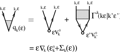
FIG. 2.: The Ward identity for the heat velocity ${\vec{q}}_{{\bf k}}({\epsilon})$ derived in this section. This identity assures that ${\vec{q}}_{{\bf k}}({\epsilon}=0)=0$.

Finally, we discuss the following two restrictions assumed in the proof of the Ward identity:

(i) In the above discussion, we assumed that the potential term in $h(z)$ is local, which is not true if the range of the interaction is finite. In this case, a correction term $C(x,y;z)$ given in eq.(C15) should be added to (43), as discussed in Appendix C. This correction term gives rise to the additional heat velocity $\Delta{\vec{q}}(k)$ given by eq.(C23). Note that $\Delta{\vec{q}}_{{\bf k}}({\epsilon})$ vanishes identically in the case of the on-site Coulomb potential. As a result, the Ward identity for the heat velocity in the case of general two-body interactions is given by

$${\vec{q}}({{\bf k}},{\epsilon})={\epsilon}{\vec{v}}_{{\bf k}}({\epsilon})+\Delta{\vec{q}}_{{\bf k}}({\epsilon}).$$ (49)

Fortunately, $\Delta{\vec{q}}(k)$ does not contribute to the transport coefficients as discussed in Appendix C. As a result, we can use the expression for ${\vec{q}}(k)$ in eq.(48) for the purpose of calculating $S$, $\kappa$ and $\nu$, even if the potential $U({{\bf k}})$ is momentum-dependent.

(ii) Here we treated the space variables like ${\bf x}$, ${\bf y}$ and ${\bf z}$ as continuous ones for the simplicity. However, it is easy to perform the similar analysis for the tight-binding model, by replacing the derivative of $\bf x$ with the differentiation. For example, the local energy conservation law is expressed as $\frac{\partial}{\partial t}h(r_{l})+(j(r_{l+1})-j(r_{l-1}))/2a=0$, where $a$ is the lattice spacing. We stress that the Ward identity in eq.(46) is rigorous also in the case of the tight-binding model. Note that we give the another proof for the Ward identity based on the diagrammatic technique in Appendix D, which is valid for general tight-binding models.

We comment that Langer studied the Ward identity for the heat velocity in ref.[15]. Unfortunately, because of a mistake, an extra factor $-{\vec{v}}_{{\bf k}}G_{{\bf k}}^{-1}({\omega})$ should be subtracted from the r.h.s. of his Ward identity (i.e., the heat velocity), eq.(3.31) in ref.[15]; see eq.(48) or (49) in the present paper. In fact, the factor ${{\bf k}}\cdot({{\bf k}}+{{\bf q}})$ in eqs. (3.16) and (3.22) (in eqs. (3.19) and (3.23)) of ref.[15] should be replaced with ${{\bf k}}^{2}$ (with $({{\bf k}}+{{\bf q}})^{2}$). This failure, which is fortunately not serious in studying the transport coefficients at lower temperatures, becomes manifest if one studies the Ward identity in terms of the $x$-representation, like in the present study.

IV Formula for the Nernst coefficient

According to the linear response theory, the Nernst coefficient is given by

$$\nu=\left[\frac{-{\alpha}_{yx}}{{\sigma}}-S\tan\theta_{\rm H}\right]/B,$$ (50)

where ${\hat{\alpha}}({\bf B})\equiv{\hat{L}}^{12}({\bf B})/T^{2}$ is called the Peltier tensor (${\vec{J}}={\hat{a}}(-{\vec{\nabla}}T)$), and $\tan\theta_{\rm H}\equiv{\sigma}_{xy}/{{\sigma}}$ is the Hall angle. Note that ${\alpha}_{yx}({\bf B})={L}_{yx}^{12}({\bf B})/T^{2}={L}_{xy}^{21}(-{\bf B})/T^{2}=-{L}_{xy}^{21}({\bf B})/T^{2}$ because of the Onsager relation. In addition, ${\alpha}_{yx}({\bf B})=-{\alpha}_{xy}({\bf B})$ in the presence of the four-fold symmetry along the magnetic filed ${\bf B}$.

In this section, we investigate the off-diagonal Peltier coefficient ${\alpha}_{yx}$ due to the Lorentz force to derive the expression for the Nernst coefficient. Up to now, the general expression for the Hall coefficient [8, 29] and that for the magnetoresistance [9] were derived by using the Fermi liquid theory based on the Kubo formula. These works enabled us to perform numerical calculations for the Hubbard model [12, 14, 31] within the conservation approximation as Baym and Kadanoff [10]. Hereafter, we derive the general expression for the Nernst coefficient by using the technique developed in refs. [8], [9] and [29].

For the present purpose, we have to include the external magnetic field. In the presence of the vector potential, the hopping parameter $t_{ij}$ in eq.(16) is multiplied by the Peierls phase factor [9]:

$$t_{ij}\rightarrow t_{ij}\exp[ie({\bf A}_{i}+{\bf A}_{j})\cdot({\bf r}_{i}-{\bf r}_{j})/2],$$ (51)

where ${\bf A}_{i}$ is the external vector potential at ${\bf r}_{i}$, and $e(<0)$ is the charge of an electron, Here we introduce ${\bf A}_{i}$ as

$${\bf A}_{i}={\bf A}e^{i{\bf p}\cdot{\bf r}_{i}},$$ (52)

where ${\bf A}$ is a constant vector. In this case, the magnetic field is given by ${\bf B}=i{\bf p}\times{\bf A}$ in the uniform limit, i.e., $|{\bf p}|\ll 1$ [8, 9, 29]. Bearing eqs.(51) and (52) in mind, the current operator defined by eq.(5) and the Hamiltonian are given by [9]

$$j_{\nu}^{B}({{\bf p}}\!=\!0) = j_{\nu}({\bf 0})-eA_{\alpha}\cdot j_{\nu{\alpha}}(-{{\bf p}}),$$ (53)

$$H_{B} = H_{B=0}-\ eA_{\alpha}j_{\alpha}(-{{\bf p}}),$$ (54)

in the tight-binding model up to $O(A)$. Here and hereafter, the summation with respect to the suffix which appears twice is taken implicitly. $j_{\alpha}({{\bf p}})$ is given in eq.(19), and

$$j_{{\alpha}{\beta}}({{\bf p}})=e\sum_{{\bf k}}(\partial_{\alpha}\partial_{\beta}{\epsilon}_{{\bf k}}^{0})c_{{{\bf k}}-{{\bf p}}/2}^{\dagger}c_{{{\bf k}}+{{\bf p}}/2}.$$ (55)

To derive the Nernst coefficient, we have to calculate the $L_{xy}^{21}$ under the magnetic field, which is given by

$$L_{xy}^{21}({{{\bf p}}},i{\omega}_{l};{\bf A})=\frac{-T}{{\omega}_{l}}\int_{0}^{\beta}d\tau e^{i{\omega}_{l}\tau}\frac{1}{Z}{\rm Tr}\left\{e^{-\beta H_{B}}T_{\tau}{j_{x}^{Q}}^{B}({{{\bf p}}},\tau)j_{y}^{B}({\bf 0},0)\right\},$$ (56)

and take derivative of eq.(56) with respect to $q_{\rho}$ and $A_{\sigma}$ up to the first order. $Z$ is the partition function. By taking eqs.(53) and (54) into account, the $A_{\sigma},q_{\rho}$-derivative of $L_{xy}^{12}({{{\bf p}}},i{\omega}_{l};{\bf A})$ is given by

$$-{\alpha}_{yx}(i{\omega}_{l}) \equiv \sum_{{\sigma}\rho}C_{xy}^{\rho{\sigma}}(i{\omega}_{l})(ip_{\rho}\cdot A_{\sigma}),$$ (57)

$$C_{xy}^{\rho{\sigma}}(i{\omega}_{l}) \equiv \left.\frac{-i}{T^{2}}\frac{\partial^{2}}{\partial p_{\rho}\partial A_{\sigma}}L_{xy}^{21}({{{\bf p}}},{\omega}_{l};{\bf A})\right|_{{\bf p}={\bf A}=0}.$$ (58)

Below, we see that the dc-Peltier coefficient ${\alpha}_{yx}$ is given by the analytic continuation of ${\alpha}_{yx}(i{\omega}_{l})$.

The diagrammatic expression for $C_{xy}^{\rho{\sigma}}(i{\omega}_{l})$ is very complicated, containing six-point vertices. Fortunately, as for the most divergent term with respect to $\gamma^{-1}$, they can be collected into a small number of simpler diagrams as shown in fig.3 by taking the Ward identity into account [8, 9, 29]. We can perform the present calculation for $C_{xy}^{\rho{\sigma}}(i{\omega}_{l})$ in a similar way to that for ${\sigma}_{xy}$ in ref. [8], only by replacing ${j}_{\mu=x}$ with ${j}^{Q}_{\mu=x}$ and using the Ward idntity for the heat velocity. As a result, we obtain the following result:

$$C_{xy}^{\rho{\sigma}}(i{\omega}_{l}) = \frac{ie^{2}}{{\omega}_{l}}\sum_{{{\bf k}},i{\epsilon}_{n}}{\Lambda}_{{{\bf k}}x}^{Q}(i{\epsilon}_{n};i{\omega}_{l})\left\{[G{{\raisebox{-1.50696pt}[-6.45831pt]{$\;\stackrel{{\scriptstyle\leftrightarrow}}{{\partial}}\!\!\!\;$}}}_{\rho}G^{+}]\partial_{\sigma}-[G{{\raisebox{-1.50696pt}[-6.45831pt]{$\;\stackrel{{\scriptstyle\leftrightarrow}}{{\partial}}\!\!\!\;$}}}_{{\sigma}}G^{+}]\partial_{\rho}\right\}\Lambda_{{{\bf k}}y}(i{\epsilon}_{n};i{\omega}_{l})$$ (60)

$$+\frac{ie^{2}}{{\omega}_{l}}\sum_{{{\bf k}},i{\epsilon}_{n}}{\Lambda}_{{{\bf k}}x}^{Q}(i{\epsilon}_{n};i{\omega}_{l})[\partial_{\rho}G^{+}\cdot\partial_{{\sigma}}G-\partial_{{\sigma}}G^{+}\cdot\partial_{\rho}G]\Lambda_{{{\bf k}}y}(i{\epsilon}_{n};i{\omega}_{l}),$$

where $G^{+}\equiv G_{{\bf k}}({\epsilon}_{l}+{\omega}_{l})$, $G\equiv G_{{\bf k}}({\epsilon}_{l})$, and $[A{{\raisebox{-1.50696pt}[-6.45831pt]{$\;\stackrel{{\scriptstyle\leftrightarrow}}{{\partial}}\!\!\!\;$}}}_{\alpha}B]\equiv A\!\cdot\!\partial_{\alpha}B-B\!\cdot\!\partial_{\alpha}A$. ${\Lambda}_{{{\bf k}}x}^{Q}(i{\epsilon}_{n};i{\omega}_{l})$ is the three point vertex for the heat current given in eq.(33). Equation (60) is described in (a)-(d) fig.3. Here, we neglect the diagrams (e) and (f) because their contribution is less singular with respect to $\gamma^{-1}$ [8].

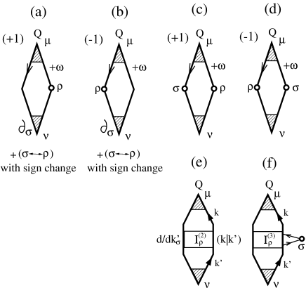
FIG. 3.:

All the diagrams for ${\alpha}_{\mu\nu}$. The symbol “$\circ\rho$” on each line represents the momentum derivative, “$\partial_{\rho}$”. The notations in the diagrams are explained in ref.[9] in detail.

Here, we assume that the magnetic field ${\bf B}$ is parallel to the $z$-axis. Then, we can easily check that $C_{xy}^{\rho{\sigma}}(i{\omega}_{l})$ in eq.(60) is expressed as $C_{xy}^{\rho=x,{\sigma}=y}(i{\omega}_{l})\cdot{\epsilon}_{z\rho{\sigma}}$. This fact assures that ${\alpha}_{xy}(i{\omega}_{l})$ given in eq.(58) is gauge-invariant, that is,

$$-{\alpha}_{yx}(i{\omega}_{l})=C_{xy}^{\rho=x,{\sigma}=y}(i{\omega}_{l})\cdot B_{z}.$$ (61)

We note that eq.(60) is equivalent to ${\sigma}_{xy}(i{\omega}_{l})/T$ if $\Lambda_{{{\bf k}}y}^{Q}$ is replaced with $\Lambda_{{{\bf k}}y}$; see “A” and “B” in p.632 of ref. [8].

In performing the analytic continuation of eq.(60), the most divergent term with resect to $\gamma^{-1}$ is given by the replacements $G({\epsilon}_{n}+{\omega}_{l})\rightarrow G^{\rm R}$ and $G({\epsilon}_{n})\rightarrow G^{\rm A}$. Taking account of the relation $\partial_{\rho}G^{\rm R}({\epsilon})=G^{\rm R}({\epsilon})^{2}(v_{{{\bf k}}\rho}({\epsilon})-i\partial_{\rho}\gamma_{{\bf k}}({\epsilon}))$, the dc-Peltier coefficient ${\alpha}_{xy}({\omega}+i\delta)|_{{\omega}=0}$ is obtained as

$$-{\alpha}_{yx} = B\cdot\frac{e^{2}}{T}\sum_{{\bf k}}\int\frac{d{\epsilon}}{\pi}\left(-\frac{\partial f}{\partial{\epsilon}}\right)\bigg{\{}|{\rm Im}G_{{\bf k}}({\epsilon})||G_{{\bf k}}({\epsilon})|^{2}Q_{{{\bf k}}x}[v_{{{\bf k}}x}\partial_{y}-v_{{{\bf k}}y}\partial_{x}]J_{{{\bf k}}y}$$ (63)

$$+|G_{{\bf k}}({\epsilon})|^{4}Q_{{{\bf k}}x}J_{{{\bf k}}y}[-v_{{{\bf k}}x}\partial_{y}\gamma_{{{\bf k}}}+v_{{{\bf k}}y}\partial_{x}\gamma_{{{\bf k}}}]\bigg{\}},$$

where ${\vec{Q}}_{{{\bf k}}}({\epsilon})$ is the total heat current introduced in eq.(35) We stress that ${\vec{Q}}_{{{\bf k}}}({\epsilon}=0)=0$ at $T=0$, as is discussed in §II.

It is instructive to make a comparison between ${\alpha}_{xy}$ and ${\sigma}_{xy}/eT$: The latter is given by eq.(63) by replacing $Q_{x}$ with $J_{x}$. In this case, the second term of eq.(63), which contains the $k$-derivative of $\gamma_{{\bf k}}$, vanishes identically because of the Onsager relation ${\sigma}_{xy}({\bf B})=-{\sigma}_{yx}({\bf B})$. As a result, the general expression for ${\sigma}_{xy}$ given in eq.(3.38) of ref. [8] is reproduced.

If the system has the four-fold symmetry along the $z$-axis, then ${\alpha}_{xy}({\bf B})=-{\alpha}_{yx}({\bf B})$. In this case, considering that $|{\rm Im}G_{{\bf k}}({\epsilon})||G_{{\bf k}}({\epsilon})|^{2}=|G_{{\bf k}}({\epsilon})|^{4}\gamma_{{\bf k}}$, eq.(63) can be rewritten as [12, 13]

$$-{\alpha}_{yx}={\alpha}_{xy} = B\cdot\frac{e^{2}}{T}\sum_{{\bf k}}\int\frac{d{\epsilon}}{2\pi}\left(-\frac{\partial f}{\partial{\epsilon}}\right)|{\rm Im}G_{{\bf k}}({\epsilon})||G_{{\bf k}}({\epsilon})|^{2}\gamma_{{\bf k}}({\epsilon})A_{{\bf k}}({\epsilon}),$$ (64)

$$A_{{\bf k}}({\epsilon}) = \left({\vec{Q}}_{{{\bf k}}}({\epsilon})\times({\vec{v}}_{{\bf k}}({\epsilon})\times{\vec{\nabla}})_{z}\left({\vec{J}}_{{{\bf k}}}({\epsilon})/\gamma_{{\bf k}}({\epsilon})\right)\right)_{z}$$ (65)

$$= |{\vec{v}}_{{{\bf k}}}({\epsilon})|_{\perp}\left({\vec{Q}}_{{{\bf k}}}({\epsilon})\times\frac{\partial}{\partial k_{\parallel}}\left({\vec{J}}_{{{\bf k}}}({\epsilon})/\gamma_{{\bf k}}({\epsilon})\right)\right)_{z},$$ (66)

where $|{\vec{v}}_{{{\bf k}}}|_{\perp}=\sqrt{v_{{{\bf k}}x}^{2}+v_{{{\bf k}}x}^{2}}$, and $k_{\parallel}$ is the momentum on the $xy$-plane along the Fermi surface, i.e., along the vector ${\vec{e}}_{\parallel}=({\vec{e}}_{z}\times{\vec{v}}_{{\bf k}})/|{\vec{v}}_{{{\bf k}}}|_{\perp}$. As noted above, eq.(64) becomes ${\sigma}_{xy}/eT$ by replacing $Q_{x}$ with $J_{x}$; see eq.(22) in ref. [12].

It is notable that $A_{{\bf k}}({\epsilon})$ in eq.(66) is rewritten as

$$(\gamma_{{\bf k}}({\epsilon})/|{\vec{v}}|_{\perp})A_{{\bf k}}({\epsilon}) = (Q_{{{\bf k}}x}J_{{{\bf k}}x}+Q_{{{\bf k}}y}J_{{{\bf k}}y})\frac{\partial\theta_{{\bf k}}^{J}}{\partial k_{\parallel}}+\left({\vec{Q}}_{{\bf k}}\times{\vec{J}}_{{\bf k}}\right)_{z}\frac{\partial}{\partial k_{\parallel}}\log(|{\vec{J}}_{{\bf k}}|/\gamma_{{\bf k}}),$$ (67)

where $\theta_{{\bf k}}^{J}=\tan^{-1}(J_{{{\bf k}}x}/J_{{{\bf k}}y})$. In an interacting system without rotational symmetry, the second term with $k_{\parallel}$-derivative of $\gamma_{{\bf k}}$ does not vanish in general since ${\vec{J}}$ is not parallel to ${\vec{Q}}$ owing to the VC’s by ${\cal T}^{22}$. In contrast, ${\vec{v}}_{{\bf k}}({\epsilon})={\vec{q}}_{{\bf k}}({\epsilon})/{\epsilon}$ because of the Ward identity. In ref. [21], based on the fluctuation-exchange (FLEX)+T-matrix approximation, we studied the Nernst coefficient of the square lattice Hubbard model as an effective model for high-$T_{c}$ cuprates. We found that the second term of eq.(67) gives the huge contribution in the pseudo-gap region if the VC’s for currents are taken into account in a conserving way. As a result, the origin of the abrupt increase of the Nernst coefficient under the pseudo-gap temperature is well understood.

V Discussions

A Vertex Correction for Thermal Conductivity

In previous sections, we studied various analytical properties for ${\vec{q}}_{{\bf k}}({\epsilon})$ or ${\vec{Q}}_{{\bf k}}({\epsilon})$, using the Ward identity for the heat velocity derived in §III. In this subsection, we study a free dispersion model (${\epsilon}_{{\bf k}}={{\bf k}}^{2}/2m$) in the presence of the electron-electron interaction without Umklapp processes. This situation will be realized in a tight-binding Hubbard model when the density of carrier is low; $n\ll 1$. Here, we explicitly calculate the total heat current ${\vec{Q}}_{{\bf k}}({\epsilon})$ in terms of the conserving approximation. The present result explicitly shows that ${\vec{J}}_{{\bf k}}({\epsilon})\neq{\vec{Q}}_{{\bf k}}({\epsilon})/{\epsilon}$.

Next, as a useful application of the expression for the transport coefficients derived in previous sections, we study the thermal conductivity $\kappa$ in a free-dispersion model. Because of the absence of Umklapp processes, the ($T^{2}$-term of the) resistivity $\rho$ of this system should be zero even at finite temperatures. In a microscopic study based on the Kubo formula, this physical requirement is recovered by taking account of all the VC’s for the current given by the Ward identity [7]. On the other hand, the thermal conductivity is finite even in the absence of the Umklapp processes because heat currents are not conserved in the elastic normal scattering processes. Hereafter, we derive the $T\gamma^{-1}$-linear term of $\kappa$ in the free dispersion model in terms of the conserving approximation. For this purpose, we can drop the second term of eq.(14) because $L^{12}L^{21}/T^{2}L^{11}=TS^{2}{\sigma}\sim O(T^{3}\gamma^{-1})$. The obtained result is exact within the second order perturbation with respect to $U$.

First we consider the second order VC’s as shown in fig.4. Because ${\vec{Q}}_{{\bf k}}({\epsilon}=0)=0$, we can write ${\vec{Q}}_{{\bf k}}({\epsilon})={\vec{C}}_{{\bf k}}\cdot{\epsilon}$ up to $O({\epsilon})$. The correction terms given by (a-c) in fig.4, $\Delta{\vec{Q}}_{{\bf k}}^{\mbox{(a-c)}}({\epsilon})$, are given by

$$\Delta{\vec{Q}}_{{\bf k}}^{(r)}({\epsilon})=U^{2}\sum_{{{\bf k}}^{\prime}}\int\frac{d{\epsilon}^{\prime}}{4}\left[{\rm cth}\frac{{\epsilon}^{\prime}-{\epsilon}}{2T}-{\rm th}\frac{{\epsilon}^{\prime}}{2T}\right]{T}_{{{\bf k}},{{\bf k}}^{\prime}}^{(r)}({\epsilon},{\epsilon}^{\prime})|G_{{{\bf k}}^{\prime}}({\epsilon}^{\prime})|^{2}{\vec{Q}}_{{{\bf k}}^{\prime}}({\epsilon}^{\prime}),$$ (68)

where $r=a,b,c$. ${T}_{{{\bf k}},{{\bf k}}^{\prime}}^{(r)}({\epsilon},{\epsilon}^{\prime})$ is a VC which is classified as ${\cal T}^{22}$: Their functional form are given by

$${T}_{{{\bf k}},{{\bf k}}^{\prime}}^{(a)}({\epsilon},{\epsilon}^{\prime}) = \frac{2}{\pi}{\rm Im}\chi_{{{\bf k}}-{{\bf k}}^{\prime}}^{0R}({\epsilon}-{\epsilon}^{\prime})$$ (69)

$$= \sum_{{\bf p}}\int d{\omega}\left[-{\rm th}\frac{{\omega}+{\epsilon}}{2T}+{\rm th}\frac{{\omega}+{\epsilon}^{\prime}}{2T}\right]\rho_{{{\bf k}}+{{\bf p}}}({\epsilon}+{\omega})\rho_{{{\bf k}}^{\prime}+{{\bf p}}}({\epsilon}^{\prime}+{\omega}),$$ (70)

$${T}_{{{\bf k}},{{\bf k}}^{\prime}}^{(b)}({\epsilon},{\epsilon}^{\prime}) = {\cal T}_{{{\bf k}},{{\bf k}}^{\prime}}^{(a)}({\epsilon},{\epsilon}^{\prime}),$$ (71)

$${T}_{{{\bf k}},{{\bf k}}^{\prime}}^{(c)}({\epsilon},{\epsilon}^{\prime}) = \sum_{{\bf p}}\int d{\omega}\left[{\rm th}\frac{{\omega}+{\epsilon}}{2T}-{\rm th}\frac{{\omega}-{\epsilon}^{\prime}}{2T}\right]\rho_{{{\bf k}}+{{\bf p}}}({\epsilon}+{\omega})\rho_{{{\bf k}}^{\prime}+{{\bf p}}}({\epsilon}^{\prime}-{\omega}),$$ (72)

where $\rho_{{{\bf k}}}({\epsilon})=\frac{1}{\pi}{\rm Im}G_{{\bf k}}({\epsilon}-i\delta)$ and $|G_{{\bf k}}({\epsilon})|^{2}=\pi\rho_{{\bf k}}({\epsilon})/\gamma_{{\bf k}}({\epsilon})$. By expanding eq.(68) with respect to ${\epsilon}$ and $T$ up to $O({\epsilon}^{2},T^{2})$ as was discussed in ref. [7] and noticing that $\displaystyle\left.\frac{\partial}{\partial{\epsilon}}\int d{\epsilon}^{\prime}[{\rm cth}\frac{{\epsilon}^{\prime}-{\epsilon}}{2T}-{\rm th}\frac{{\epsilon}^{\prime}}{2T}]({\epsilon}^{\prime}-{\epsilon}){\epsilon}^{\prime}\right|_{{\epsilon}=0}=\frac{1}{3}(\pi T)^{2}$, we obtain that

$$\Delta{\vec{Q}}_{{\bf k}}^{(a)} = \frac{{\epsilon}}{3}U^{2}\sum_{{{\bf k}}^{\prime}{{\bf p}}}\pi\rho_{{{\bf k}}+{{\bf p}}}(0)\rho_{{{\bf k}}^{\prime}+{{\bf p}}}(0)\rho_{{{\bf k}}^{\prime}}(0)\frac{{{\epsilon}}^{2}+(\pi T)^{2}}{2\gamma_{{{\bf k}}^{\prime}}({\epsilon})}{\vec{C}}_{{{\bf k}}^{\prime}},$$ (73)

$$\Delta{\vec{Q}}_{{\bf k}}^{(b)} = \Delta{\vec{Q}}_{{\bf k}}^{(a)},$$ (74)

$$\Delta{\vec{Q}}_{{\bf k}}^{(c)} = -\Delta{\vec{Q}}_{{\bf k}}^{(a)}.$$ (75)

In deriving eq.(75), we have changed the integration variables $({{\bf k}}^{\prime},{\epsilon}^{\prime})\rightarrow(-{{\bf k}}^{\prime},-{\epsilon}^{\prime})$, and used the relation $\rho_{-{{\bf k}}}(0)=\rho_{{{\bf k}}}(0)$ and ${\vec{Q}}_{-{{\bf k}}}(-{\epsilon})={\vec{Q}}_{{{\bf k}}}({\epsilon})$. In general, within the FLEX approximation, the Aslamazov-Larkin (AL) type VC’s by ${\cal T}^{22}$, which correspond to (b) and (c), turn out to cancel out for the heat current.

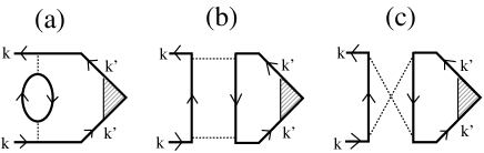
FIG. 4.: The vertex corrections (by ${\cal T}_{22}$) for the heat/electron current in the second order perturbation theory.

In the same way, the imaginary part of the self-energy, $\gamma_{{\bf k}}({\epsilon})$, is given by

$$\gamma_{{\bf k}}({\epsilon})=({{\epsilon}}^{2}+(\pi T)^{2})\frac{U^{2}}{2}\sum_{{{\bf k}}^{\prime}{{\bf p}}}\pi\rho_{{{\bf k}}+{{\bf p}}}(0)\rho_{{{\bf k}}^{\prime}+{{\bf p}}}(0)\rho_{{{\bf k}}^{\prime}}(0),$$ (76)

which is shown in fig.5.

FIG. 5.: The self-energy given by the second order perturbation.

In a spherical system, we can put ${\vec{C}}_{{\bf k}}={C}\frac{{{\bf k}}^{\prime}}{k_{\rm F}}$ on the Fermi surface. Then, the total correction for ${\vec{Q}}$ is given by

$$\Delta{\vec{Q}}_{{\bf k}} \equiv \sum_{r}^{a,b,c}\Delta{\vec{Q}}_{{\bf k}}^{(r)}$$ (77)

$$= \frac{{\epsilon}}{3Z}\sum_{{{\bf k}}^{\prime}{{\bf p}}}\rho_{{{\bf k}}+{{\bf p}}}(0)\rho_{{{\bf k}}^{\prime}+{{\bf p}}}(0)\rho_{{{\bf k}}^{\prime}}(0)\cdot{C}\frac{{{\bf k}}^{\prime}}{k_{\rm F}},$$ (78)

$$Z = \sum_{{{\bf k}}^{\prime}{{\bf p}}}\rho_{{{\bf k}}+{{\bf p}}}(0)\rho_{{{\bf k}}^{\prime}+{{\bf p}}}(0)\rho_{{{\bf k}}^{\prime}}(0).$$ (79)

Here, we put ${{\bf k}}=(0,0,k_{\rm F})$. Then, the $z$-component of eq.(78) is given by

$$C\frac{{\epsilon}}{3Z}\int dk^{\prime}d\theta_{k^{\prime}}d\phi_{k^{\prime}}\int dpd\theta_{p}d\phi_{p}{k^{\prime}}^{2}p^{2}\sin\theta_{k^{\prime}}\sin\theta_{p}\cdot\delta({\epsilon}_{{{\bf k}}^{\prime}}-\mu)\delta({\epsilon}_{{{\bf k}}+{{\bf p}}}-\mu)\delta({\epsilon}_{{{\bf k}}^{\prime}+{{\bf p}}}-\mu)\cdot\cos\theta_{k^{\prime}}.$$ (80)

Note that in a free dispersion model, $\rho_{{\bf k}}(0)=z\delta(z({\epsilon}_{{\bf k}}-\mu))=\delta({\epsilon}_{{\bf k}}-\mu)$, where ${\epsilon}_{{\bf k}}={{\bf k}}^{2}/2m$ and $z$ is the renormalization factor. By performing $k^{\prime}$-integration, $\theta_{p}$-integration, and $\phi_{p},\phi_{k^{\prime}}$-integrations successively, eq.(80) becomes

$$C\frac{4\pi z^{3}{m}^{3}{\epsilon}}{3Z}\int d\theta_{k^{\prime}}\int_{0}^{2k_{F}^{2}\sin^{2}\theta_{k^{\prime}}/(1-\cos\theta_{k^{\prime}})}dp\frac{\sin\theta_{k^{\prime}}\cos\theta_{k^{\prime}}}{\sqrt{4k_{F}^{2}\sin^{2}\theta_{k^{\prime}}-2p^{2}(1-\cos\theta_{k^{\prime}})}}$$ (81)

$$=C\frac{4\pi{m}^{3}{\epsilon}}{3Z}\int_{0}^{\pi}d\theta_{k^{\prime}}\frac{\sin\theta_{k^{\prime}}\cos\theta_{k^{\prime}}}{\sqrt{2(1-\cos\theta_{k^{\prime}})}}=C\frac{8\pi m^{3}{\epsilon}}{9Z}.$$ (82)

In the same way, $Z$ is calculated as

$$Z = 4\pi{m}^{3}\int_{0}^{\pi}d\theta_{k^{\prime}}\frac{\sin\theta_{k^{\prime}}}{\sqrt{2(1-\cos\theta_{k^{\prime}})}}$$ (83)

$$= 8\pi m^{3}.$$ (84)

As a result, $\Delta{\vec{Q}}_{{\bf k}}$ is given by

$$\Delta{\vec{Q}}_{{\bf k}}=\frac{{\epsilon}}{9}C\frac{{{\bf k}}}{k_{\rm F}}=\frac{1}{9}{\vec{Q}}_{{{\bf k}}}.$$ (85)

By solving the Bethe-Salpeter equation, ${\vec{Q}}={\vec{q}}+\Delta{\vec{Q}}$, we get

$${\vec{Q}}_{{\bf k}}=\frac{9}{8}{\vec{q}}_{{\bf k}},$$ (86)

where ${\vec{q}}_{{\bf k}}={\epsilon}{\vec{v}}_{{\bf k}}$. As a result, the thermal conductivity within the second-order perturbation theory is given by

$$\kappa=\frac{9}{8}\kappa^{0},$$ (87)

$$\kappa^{0}=\frac{\pi^{2}nk_{B}^{2}T}{6m\gamma},$$ (88)

where $\kappa^{0}$ is the result of the RTA, where VC’s are neglected. Note that $m$ in eq.(88) is unrenormalized, and $n$ is the number of electrons in a unit volume. Finally, performing the momentum summations in eq.(76), $\gamma$ of order $U^{2}$ is given by

$$\gamma=({\epsilon}^{2}+(\pi T)^{2})\frac{U^{2}m^{3}}{2\pi}.$$ (89)

In conclusion, the vertex corrections slightly enhances (by $\frac{9}{8}$ times) the thermal conductivity in a three-dimensional free-dispersion model within the second order perturbation theory.

It is instructive to make a comparison between the role of VC’s for the heat current and that for the electron current. The VC’s for the electron current which correspond to fig.4 (a)-(c) are given by

$$\Delta{\vec{J}}_{{\bf k}}^{(a)} = \Delta{\vec{J}}_{{\bf k}}^{(b)}=\Delta{\vec{J}}_{{\bf k}}^{(c)}$$ (90)

$$= U^{2}\sum_{{{\bf k}}^{\prime}{{\bf p}}}\pi\rho_{{{\bf k}}+{{\bf p}}}(0)\rho_{{{\bf k}}^{\prime}+{{\bf p}}}(0)\rho_{{{\bf k}}^{\prime}}(0)\frac{{{\epsilon}}^{2}+(\pi T)^{2}}{2\gamma_{{{\bf k}}^{\prime}}({\epsilon})}{\vec{J}}_{{{\bf k}}^{\prime}},$$ (91)

which was already derived in ref. [7]. Here we put ${\vec{J}}_{{{\bf k}}}=D\frac{{{\bf k}}}{k_{\rm F}}$ on the Fermi surface. Performing all the momentum integrations in the spherical case as before, we find that

$$\Delta{\vec{J}}_{{\bf k}} \equiv \sum_{r}^{a,b,c}\Delta{\vec{J}}_{{\bf k}}^{(r)}$$ (92)

$$= \frac{3}{Z}\sum_{{{\bf k}}^{\prime}{{\bf p}}}\rho_{{{\bf k}}+{{\bf p}}}(0)\rho_{{{\bf k}}^{\prime}+{{\bf p}}}(0)\rho_{{{\bf k}}^{\prime}}(0)\cdot D\frac{{{\bf k}}^{\prime}}{k_{F}}$$ (93)

$$= D\frac{{{\bf k}}}{k_{F}},$$ (94)

where $Z$ is given in eq.(79). As a result, the solution of the Bethe-Salpeter equation ${\vec{J}}={\vec{v}}+\Delta{\vec{J}}$ is given by ${\vec{J}}=\infty$, which means that the conductivity diverges in the absence of the Umklapp processes, even at finite temperatures. Thus, the important result in ref. [7] is recovered. On the other hand, the thermal conductivity does not diverge even in the absence of the Umklapp processes, because the normal scattering process attenuates the heat current.

B The TEP and the Nernst Coefficient

In this section, we discuss the effect of the anisotropy as well as the role of the VC’s for the TEP and the Nernst coefficient. First, we discuss the validity of the Mott formula for $S$ [30] which is given by

$$S = \frac{\pi^{2}k_{\rm B}^{2}T}{3e}\left[\frac{\partial\ln{\sigma}(E)}{\partial E}\right]_{E_{\rm F}}.$$ (95)

It is easy to see that eq.(95) is valid even in the presence of Coulomb interactions, if we define ${\sigma}({\epsilon})\equiv e^{2}\sum_{{\bf k}}|G_{{\bf k}}({\epsilon})|^{2}v_{{{\bf k}}x}({\epsilon})J_{{{\bf k}}x}({\epsilon})$ [3]: ${\sigma}$ and $S$ given by eqs.(26) and (36) are rewritten using ${\sigma}({\epsilon})$ as

$${\sigma} = \int\frac{d{\epsilon}}{\pi}\left(-\frac{\partial f}{\partial{\epsilon}}\right){\sigma}({\epsilon}),$$ (96)

$$S = \frac{1}{eT{\sigma}}\int\frac{d{\epsilon}}{\pi}\left(-\frac{\partial f}{\partial{\epsilon}}\right){\epsilon}{\sigma}({\epsilon}),$$ (97)

At sufficiently lower temperatures, eqs.(96) and (97) become

$${\sigma} = {\sigma}(0),$$ (98)

$$S = \frac{\pi^{2}k_{\rm B}^{2}T}{3e{\sigma}}\left.\frac{d{\sigma}({\epsilon})}{d{\epsilon}}\right|_{{\epsilon}=0}.$$ (99)

As a result, Mott formula is also satisfied in the case of electron-electron interaction. Note that the renormalization factor $z$ does not appear in eq.(95).

To analyze the TEP in more detail, we rewrite the expression for $S$ by using the quasiparticle representation of the Green function, eq.(18), which is possible at sufficiently low temperatures in the Fermi liquid. Using the relation

$$\sum_{{\bf k}} = \int dS_{k}dk_{\perp}=\int\frac{dS_{k}d{\epsilon}_{{\bf k}}^{0}}{|v_{{\bf k}}^{0}|}$$ (100)

$$= \int\frac{dS_{k}d{\epsilon}_{{\bf k}}^{\ast}}{z_{{\bf k}}|v_{{\bf k}}|},$$ (101)

where $S_{k}$ represents the Fermi surface and ${k_{\perp}}$ is the momentum perpendicular to the Fermi surface, we obtain the following expression:

$$S=\frac{e\pi^{2}k_{\rm B}^{2}T}{3{\sigma}}\frac{1}{(2\pi)^{3}}\int\frac{dS_{k}}{z_{{\bf k}}|v_{{\bf k}}|}\frac{\partial}{\partial k_{\perp}}\left\{\frac{v_{{{\bf k}}x}J_{{{\bf k}}x}}{|{\vec{v}}_{{\bf k}}|\gamma_{{\bf k}}}\right\}_{{\epsilon}={\epsilon}_{{\bf k}}^{\ast}},$$ (102)

where we performed the ${\epsilon}$-integration first by assuming the relation $\gamma\ll T$. In an anisotropic system, the ${{\bf k}}$-dependence of the integrand in eq.(102) may be strong. In high-$T_{\rm c}$ cuprates, for example, it is known that the anisotropy of $\gamma_{{\bf k}}(0)$ on the Fermi surface is very large because of the strong antiferromagnetic fluctuations. The point on the Fermi surface where $\gamma_{{\bf k}}$ takes its minimum value is called the “cold spot”, and the electrons around the cold spot mainly contribute to the transport phenomena. Because $\gamma_{{\bf k}}({\epsilon}_{{\bf k}}^{\ast})$ has a huge $k_{\perp}$-dependence in high-$T_{\rm c}$ cuprates around the cold spot, the sign of $S$ is almost determined by the sign of $e\frac{\partial\gamma_{{\bf k}}^{-1}({\epsilon}_{{\bf k}}^{\ast})}{\partial k_{\perp}}$ at the cold spot [31].

Next, we discuss the Nernst coefficient. Within the RTA, the Nernst coefficient is derived from eqs.(63), (34) and (36) by dropping all the VC’s by ${\cal T}^{22}$. In an isotropic system, $\nu$ by RTA is expressed in a simple form as [32, 33]

$$\nu_{\rm RTA} = \frac{\pi^{2}k_{\rm B}^{2}T}{3m}\left[\frac{\partial\tau(E)}{\partial E}\right]_{E_{\rm F}},$$ (103)

where $\tau({\epsilon})=1/2\gamma({\epsilon})$ is the energy-dependent relaxation time and $E_{\rm F}$ is the Fermi energy. According to eq.(103), $\nu$ is determined by the energy-dependence of the relaxation time.

Unfortunately, eq. (103) will be too simple to analyze realistic metals with (strong) anisotropy. For that purpose, we perform the ${\epsilon}$-integration of ${\alpha}_{xy}$ in eq.(64) by using the quasiparticle representation. The obtained expression for ${\alpha}_{xy}$ is given by

$${\alpha}_{xy}=B\frac{e^{2}\pi^{2}k_{\rm B}^{2}T}{12}\frac{1}{(2\pi)^{3}}\int\frac{dS_{k}}{z_{{\bf k}}|v_{{\bf k}}|}\frac{\partial}{\partial k_{\perp}}\left\{\left({\vec{Q}^{\prime}}_{{\bf k}}\times\frac{\partial}{\partial k_{\parallel}}\left(\frac{{\vec{J}}_{{\bf k}}}{\gamma_{{\bf k}}}\right)\right)_{z}\frac{|{\vec{v}}_{{\bf k}}|_{\perp}}{|{\vec{v}}_{{\bf k}}|\gamma_{{\bf k}}}\right\}_{{\epsilon}={\epsilon}_{{\bf k}}^{\ast}},$$ (104)

where ${\vec{Q}^{\prime}}_{{\bf k}}({\epsilon})\equiv{\vec{Q}}_{{\bf k}}({\epsilon})/{\epsilon}$ at zero temperature. We stress that ${\vec{Q}^{\prime}}_{{\bf k}}({\epsilon}=0)$ is finite at $T=0$ as explained is §II, which leads to the relation $\nu\sim O(T\gamma^{-1})$. We stress that ${\vec{Q}^{\prime}}_{{\bf k}}(0)$ is not equal to ${\vec{J}}_{{\bf k}}(0)$ in general, because the VC’s for heat current and the electron one work in a different way; see discussions in §IV and §V A.

We also comment that the Mott formula type expression for ${\alpha}_{xy}$,

$${\alpha}_{xy}{{\raisebox{-1.50696pt}[-6.45831pt]{$\;\stackrel{{\scriptstyle{\mbox{RTA}}}}{{=}}\;$}}}\frac{\pi^{2}k_{\rm B}^{2}T}{3e}\left[\frac{\partial{\sigma}_{xy}(E)}{\partial E}\right]_{E_{\rm F}}$$ (105)

is obtained within the RTA, by assuming that ${\vec{Q}}_{{\bf k}}({\epsilon})={\epsilon}{\vec{J}}_{{\bf k}}({\epsilon})$. This assumption, however, will be totally violated once we take the VC’s into account. As a result, eq.(105) is no more valid in a correlated electron system.

Finally, we discuss the Nernst coefficient in high-$T_{c}$ cuprates which increases drastically below the pseudo-gap temperature, $T^{\ast}$. According to the numerical analysis based on the conserving approximation [21], $k_{\parallel}$-dependence of $|{\vec{J}}_{{\bf k}}|$ becomes huge due to the VC caused by the strong superconducting fluctuations. Moreover, ${\vec{Q}}_{{\bf k}}\times{\vec{J}}_{{\bf k}}$ is large because the VC is much effective only for ${\vec{J}}_{{\bf k}}$. By considering eq.(67), the growth of the Nernst coefficient in high-$T_{c}$ cuprates under $T^{\ast}$ is caused by the enhancement of $\frac{\partial}{\partial k_{\parallel}}|{\vec{J}}_{{\bf k}}|$, not by $\frac{\partial}{\partial E}\tau(E)$ [21].

VI Summary

In the present paper, we have derived the general expressions for $S$, $\kappa$ and $\nu$ in the presence of electron-electron interactions based on the linear response theory for the thermoelectric transport phenomena. Each expression is “exact” as for the most divergent term with respect to $\gamma^{-1}$. The heat velocity ${\vec{q}}_{{\bf k}}({\epsilon})$, which is required to calculate $S$, $\kappa$ and $\nu$, is given by the Ward identity with respect to the local energy conservation law. We have studied the analytical properties of ${\vec{q}}_{{\bf k}}({\epsilon})$ as well as the total heat current ${\vec{Q}}_{{\bf k}}({\epsilon})$ in detail.

The expressions for $S$, $\kappa$ and $\nu$ derived in the present paper are summarized as follows. Note that they are valid even if the Coulomb potential $U({{\bf k}})$ has a momentum-dependence, as discussed in Appendix C. Here, $e(<0)$ is the charge of an electron.

(i) TEP: It is better to include the “incoherent correction”, which will be important in strongly correlated systems, as is discussed in ref. [34]. As a result, the final expression for $S$ is given by

$$S=\frac{e}{T{\sigma}}\sum_{{\bf k}}\int\frac{d{\epsilon}}{\pi}\left(-\frac{\partial f}{\partial{\epsilon}}\right)q_{{{\bf k}}x}({\epsilon})\left[\ |G_{{\bf k}}({\epsilon})|^{2}J_{{{\bf k}}x}({\epsilon})-{\rm Re}\{G_{{\bf k}}^{2}({\epsilon})\}v_{{{\bf k}}x}({\epsilon})\ \right],$$ (106)

where ${\sigma}={\sigma}_{xx}$ is the electric conductivity, ${\vec{v}}_{{\bf k}}({\epsilon})={\vec{\nabla}}_{k}({\epsilon}_{{\bf k}}^{0}+{\rm Re}\Sigma_{{\bf k}}({\epsilon}))$, ${\vec{q}}_{{\bf k}}({\epsilon})={\epsilon}{\vec{v}}_{{\bf k}}({\epsilon})$, and the total electron current ${\vec{J}}_{{{\bf k}}}({\epsilon})$ is given in eq.(27).

(ii) Thermal conductivity: In the same way, we include the incoherent correction. Then, the final expression for $\kappa$ is given by

$$\kappa = \frac{1}{T}\sum_{{\bf k}}\int\frac{d{\epsilon}}{\pi}\left(-\frac{\partial f}{\partial{\epsilon}}\right)q_{{{\bf k}}x}({\epsilon})\left[\ |G_{{\bf k}}({\epsilon})|^{2}Q_{{{\bf k}}x}({\epsilon})-{\rm Re}\{G_{{\bf k}}^{2}({\epsilon})\}q_{{{\bf k}}x}({\epsilon})\ \right]$$ (108)

$$-TS^{2}{\sigma},$$

where ${\vec{Q}}_{{{\bf k}}}({\epsilon})$ is given in eq.(35). Note that ${\vec{Q}}_{{{\bf k}}}({\epsilon})/{\epsilon}\neq{\vec{J}}_{{{\bf k}}}({\epsilon})$, although the Ward identity ${\vec{q}}_{{{\bf k}}}({\epsilon})/{\epsilon}={\vec{v}}_{{{\bf k}}}({\epsilon})$ is rigorously satisfied.

(iii) The expression for $\nu$ is given by eq.(50), where ${\alpha}_{xy}$ is given by eq.(63) or eq.(64). As for ${\alpha}_{xy}$ (and ${\sigma}_{xy}$), no incoherent correction exists as discussed in ref. [34].

These derived expressions enable us to calculate the VC’s in the framework of the conserving approximation. In each expression, the factor 2 due to the spin degeneracy is taken into account. We note that our expression are equivalent to that of the relaxation time approximation (RTA), if we drop all the vertex corrections in the formulae. However, the RTA is dangerous because it may give unphysical results owing to the lack of conservation laws. In conclusion, the present work gives us the fundamental framework for the microscopic study of the thermoelectric transport phenomena in strongly correlated electron systems. Owing to the present work, the conserving approximation for thermoelectric transport coefficients becomes much practical on the basis of the Fermi liquid theory.

acknowledgement

The author is grateful to T. Saso, K. Yamada and K. Ueda for useful comments and discussions. He is also grateful to one of the referees for informing him of the existence of ref. [15].

A Another derivation of the heat current operator, eq.(23)

In ref. [3], the authors derived the formula for $L^{12}({\omega}_{l})$ under the condition that electron-phonon scattering and the impurity scattering exist. In this appendix, for an instructive purpose, we derive eq.(24) in §II in the case of the on-site Coulomb interaction by using the similar technique used in ref. [3] This fact means that the heat current operator in the Hubbard model can be rewritten as eq.(23).

According to the equation of motion, the following equations are satisfied:

$$\frac{\partial}{\partial\tau}c_{k{\sigma}}^{\dagger}(\tau) = [H,c_{k{\sigma}}^{\dagger}(\tau)]$$ (A1)

$$= {\epsilon}_{k}^{0}c_{k{\sigma}}^{\dagger}+\frac{U}{2}\sum_{K^{\prime}q{\sigma}}c_{k-q,{\sigma}}^{\dagger}c_{k^{\prime}+q/2,-{\sigma}}^{\dagger}c_{k^{\prime}-q/2,-{\sigma}},$$ (A2)

$$\frac{\partial}{\partial\tau}c_{k{\sigma}}(\tau) = [H,c_{k{\sigma}}(\tau)]$$ (A3)

$$= -{\epsilon}_{k}^{0}c_{k{\sigma}}^{\dagger}-\frac{U}{2}\sum_{K^{\prime}q{\sigma}}c_{k+q,{\sigma}}c_{k^{\prime}+q/2,-{\sigma}}^{\dagger}c_{k^{\prime}-q/2,-{\sigma}}.$$ (A4)

Using $j_{\mu}^{Q}$ given in eq.(21) and taking eqs. (A2) and (A4) into account, we see that

$$\left\langle T_{\tau}j_{\mu}^{Q}(\tau)j_{\nu}(0)\right\rangle = \sum_{k{\sigma}}v_{k,\mu}^{0}{\epsilon}_{k}^{0}\left\langle T_{\tau}c_{k{\sigma}}^{\dagger}(\tau)c_{k{\sigma}}(\tau)j_{\nu}(0)\right\rangle$$ (A6)

$$+\frac{U}{2}\sum_{kk^{\prime}q{\sigma}}\frac{1}{2}(v_{k+q/2,\mu}^{0}+v_{k-q/2,\mu}^{0})\left\langle T_{\tau}c_{k-q/2{\sigma}}^{\dagger}(\tau)c_{k+q/2{\sigma}}(\tau)c_{k^{\prime}+q/2,-{\sigma}}^{\dagger}(\tau)c_{k^{\prime}-q/2,-{\sigma}}(\tau)j_{\nu}(0)\right\rangle$$

$$= \lim_{\tau^{\prime}\rightarrow\tau}\frac{1}{2}\left(\frac{\partial}{\partial\tau}-\frac{\partial}{\partial\tau^{\prime}}\right)\sum_{k{\sigma}}v_{k,\mu}^{0}\left\langle T_{\tau}c_{k{\sigma}}^{\dagger}(\tau)c_{k{\sigma}}(\tau^{\prime})j_{\nu}(0)\right\rangle.$$ (A7)

By inputting the above expression in eq.(11), we can obtain the same expression as eq.(24). As a result, ${\vec{j}}^{Q}({{\bf p}}=0,{\omega}_{l})$ can be expressed as eq.(23). We note that eq. (23) is not exact in the case of the finite range interactions. Nonetheless, eq. (23) is valid for the analysis of the transport coefficient as for the most divergent term with respect to $\gamma^{-1}$, as discussed in §III or in Appendix C.

B Definition of ${\cal T}^{{lm}}({{\bf p}}{\epsilon},{{\bf p}}^{\prime}{\epsilon}^{\prime})$

Considering the convenience for readers, we list the expression for ${\cal T}^{{lm}}({{\bf p}}{\epsilon},{{\bf p}}^{\prime}{\epsilon}^{\prime})$ introduced by Eliashberg in eq.(12) of ref.[6], following the advice by referees. Here we dropped the momentum suffixes for simplicity. By taking the limit of ${\omega}\rightarrow 0$, they are given by

$${\cal T}^{11}({\epsilon},{\epsilon}^{\prime}) = {\rm th}\frac{{\epsilon}^{\prime}}{2T}\Gamma_{11}^{\mbox{I}}+{\rm cth}\frac{{\epsilon}^{\prime}-{\epsilon}}{2T}(\Gamma_{11}^{\mbox{II}}-\Gamma_{11}^{\mbox{I}}),$$ (B1)

$${\cal T}^{12}({\epsilon},{\epsilon}^{\prime}) = 0,$$ (B2)

$${\cal T}^{13}({\epsilon},{\epsilon}^{\prime}) = -{\rm th}\frac{{\epsilon}^{\prime}}{2T}\Gamma_{13}^{\mbox{I}}-{\rm cth}\frac{{\epsilon}^{\prime}+{\epsilon}}{2T}(\Gamma_{13}^{\mbox{II}}-\Gamma_{13}^{\mbox{I}}),$$ (B3)

$${\cal T}^{21}({\epsilon},{\epsilon}^{\prime}) = {\rm th}\frac{{\epsilon}^{\prime}}{2T}\Gamma_{21},$$ (B4)

$${\cal T}^{22}({\epsilon},{\epsilon}^{\prime}) = ({\rm cth}\frac{{\epsilon}^{\prime}-{\epsilon}}{2T}-{\rm th}\frac{{\epsilon}^{\prime}}{2T})\Gamma_{22}^{\mbox{II}}+({\rm cth}\frac{{\epsilon}^{\prime}+{\epsilon}}{2T}-{\rm cth}\frac{{\epsilon}^{\prime}-{\epsilon}}{2T})\Gamma_{22}^{\mbox{III}}+({\rm th}\frac{{\epsilon}^{\prime}}{2T}-{\rm cth}\frac{{\epsilon}^{\prime}+{\epsilon}}{2T})\Gamma_{22}^{\mbox{IV}},$$ (B5)

$${\cal T}^{23}({\epsilon},{\epsilon}^{\prime}) = -{\rm th}\frac{{\epsilon}^{\prime}}{2T}\Gamma_{23},$$ (B6)

$${\cal T}^{31}({\epsilon},{\epsilon}^{\prime}) = {\rm th}\frac{{\epsilon}^{\prime}}{2T}\Gamma_{31}^{\mbox{I}}+{\rm cth}\frac{{\epsilon}^{\prime}+{\epsilon}}{2T}(\Gamma_{31}^{\mbox{II}}-\Gamma_{31}^{\mbox{I}}),$$ (B7)

$${\cal T}^{32}({\epsilon},{\epsilon}^{\prime}) = 0,$$ (B8)

$${\cal T}^{33}({\epsilon},{\epsilon}^{\prime}) = -{\rm th}\frac{{\epsilon}^{\prime}}{2T}\Gamma_{33}^{\mbox{I}}-{\rm cth}\frac{{\epsilon}^{\prime}-{\epsilon}}{2T}(\Gamma_{33}^{\mbox{II}}-\Gamma_{33}^{\mbox{I}}),$$ (B9)

where $\Gamma_{lm}^{N}\equiv\Gamma_{lm}^{N}({\epsilon},{\epsilon}^{\prime})$ ($l,m=1,2,3$, $N={\rm I,II,III,IV}$) is a four-point vertex function, which is introduced by the analytic continuation of the four-point vertex function $\Gamma(i{\epsilon}_{n},i{\epsilon}_{n^{\prime}};i{\omega}_{l})$ as shown in fig. 6. For instance, $\Gamma_{11}^{\mbox{I}}({\epsilon},{\epsilon}^{\prime})$ comes from the analytic region [$(1,1),I$] in Fig. 7 (where ${\omega}_{l}>0$) and taking the limit ${\omega}\rightarrow 0$ at the final stage. There analytic properties are well studied in ref. [6].

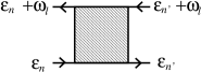
FIG. 6.: The diagrammatic expression for $\Gamma(i{\epsilon}_{n},i{\epsilon}_{n^{\prime}};i{\omega}_{l})$.

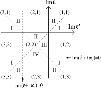
FIG. 7.: The definition of the region [$(l,m),N$].

C The Ward identity in the Case of the
Non-local Electron-Electron Interaction

In this appendix, we show that the expressions for $S$, $\kappa$ and $\nu$ derived in the present paper is valid beyond the on-site Coulomb interaction. For that purpose, we reconsider the Ward identity for the following Hamiltonian $H$ with a long-range interaction $U({\bf x}-{\bf y})$:

$$h(z) = c^{\dagger}(z)\left(\frac{-\hbar^{2}{\vec{\nabla}}^{2}}{2m}\right)c(z)+\frac{1}{2}c^{\dagger}(z)c(z)\int c^{\dagger}(r)c(r)V(z-r)d^{4}r,$$ (C1)

$$H = \int h(z)dz,$$ (C2)

where $V(x-y)\equiv U({\bf x}-{\bf y})\delta(x_{0}-y_{0})$, and $h(z)$ is the local Hamiltonian. Hereafter, we drop the spin suffixes for simplicity. In the same reason, we put $\mu=0$.

Here, it is easy to check that

$$[h(z),c(x)]\delta(z_{0}-x_{0}) = \delta^{4}(x-z)\frac{\hbar^{2}{\vec{\nabla}}^{2}}{2m}c(x)-\delta^{4}(z-x)\frac{1}{2}c(z)\int c^{\dagger}(r)c(r)V(z-r)d^{4}r$$ (C4)

$$-\frac{1}{2}c^{\dagger}(z)c(z)c^{\dagger}(z)V(z-x),$$

$$[H,c(x)] = \frac{\hbar^{2}{\vec{\nabla}}^{2}}{2m}c(x)-\int c^{\dagger}(r)c(r)V(x-r)d^{4}r\cdot c(x).$$ (C5)

By comparing eqs.(C4) and (C5) and using the kinetic equation $[H,c(x)]=-i\frac{\partial}{\partial x_{0}}c(x)$, we obtain that

$$[h(z),c(x)]\delta(z_{0}-x_{0}) = \delta^{4}(z-x)(-i)\frac{\partial}{\partial x_{0}}c(x)-\frac{1}{2}c^{\dagger}(z)c(z)c(x)V(z-x)$$ (C7)

$$+\delta^{4}(z-x)\frac{1}{2}\int c^{\dagger}(r)c(r)V(r-x)d^{4}r\cdot c(x).$$

As a result,

$$\langle T[h(z),c(x)]c^{\dagger}(y)\rangle\delta(x_{0}-z_{0}) = \delta^{4}(x-z)\frac{\partial}{\partial x_{0}}G(x-y)-Y(x,y;z)V(x-z)$$ (C9)

$$+\delta^{4}(x-z)\int Y(x,y;r)V(x-r)d^{4}r,$$

where $T$ is a time-ordering operator, and

$$Y(x,y;z) \equiv \frac{1}{2}\langle Tc^{\dagger}(z)c(z)c(x)c^{\dagger}(y)\rangle$$ (C10)

$$= \frac{1}{2}\int\!\!\int G(x,x^{\prime})\Lambda_{0}(x^{\prime},y^{\prime},z)G(y^{\prime},y)d^{4}x^{\prime}d^{4}y^{\prime},$$ (C11)

where $\Lambda_{0}(x^{\prime},y^{\prime},z)$ is the three-point vertex function for the electron density; $\rho(z)=c^{\dagger}(z)c(z)$. In the same way,

$$\langle Tc(x)[h(z),c^{\dagger}(y)]\rangle\delta(y_{0}-z_{0}) = \delta^{4}(y-z)\frac{\partial}{\partial y_{0}}G(x-y)-Y(x,y;z)V(y-z)$$ (C13)

$$+\delta^{4}(y-z)\int Y(x,y;r)V(y-r)d^{4}r.$$

As a result, we find that the following correction term

$$C(x,y;z) = -Y(x,y;z)(V(x-z)+V(y-z))$$ (C15)

$$+\int Y(x,y;r)(\delta^{4}(x-z)V(x-r)+\delta^{4}(y-z)V(y-r))d^{4}r$$

is added to eq.(43) when $U(x-y)$ is a finite-range potential. It is easy to see that $C(x,y;z)=0$ if the potential is local (i.e., $U(x-y)=U_{0}\delta({\bf x}-{\bf y})$).

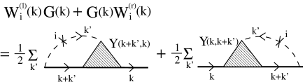
FIG. 8.:

The diagrammatic expression for eq.(C20).

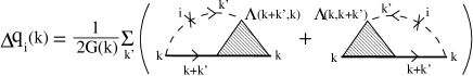
FIG. 9.:

The diagrammatic expression for $\Delta{\vec{q}}(k)$ given by eq.(C23).

Now, we take the Fourier transformation of $C(x,y;z)$ according to eq.(39). If we put $p_{\mu}=0$ for $\mu\neq i$ ($i$=1,2 or 3) and $|p_{i}|\ll 1$, $C(k;k+p_{i})$ is given by

$$C(k;k+p_{i}) \equiv \int d^{4}xd^{4}yd^{4}z\ C(x,y;z)e^{ik(x-y)+ip(x-z)}$$ (C16)

$$= ip_{i}\int d^{4}xd^{4}yd^{4}z\ Y(x,y;z)\left[V(x-z)\cdot(x_{i}-z_{i})+V(y-z)\cdot(y_{i}-z_{i})\right]e^{ik(x-y)}$$ (C18)

$$+O(p_{i}^{2}).$$

Because the Fourier transformation of $V(x)\cdot x_{i}$ is given by $-i\frac{\partial U(k)}{\partial k_{i}}$,

$$\lim_{p_{i}\rightarrow 0}\frac{C(k;k+p_{i})}{ip_{i}} = \int d^{4}k^{\prime}\left(Y(k+k^{\prime};k)+Y(k;k+k^{\prime})\right)(-i)\frac{\partial}{\partial k_{i}^{\prime}}U(k^{\prime})$$ (C19)

$$\equiv \frac{1}{2}\left(W_{i}^{(l)}(k)G(k)+G(k)W_{i}^{(r)}(k)\right),$$ (C20)

which is diagrammatically shown in fig. 8. $W_{i}^{(l)}(k)$ and $W_{i}^{(r)}(k)$ are introduced in the last line of eq.(C20).

Here we note that the energy dependence of $W_{i}^{(l,r)}(k)$ around the Fermi level is same as that of $\Sigma(k)$, that is, ${\rm Re}W_{i}(k)\sim{\rm const.}$ and ${\rm Im}W_{i}(k)\approx k_{0}^{2}$ for $|k_{0}|\ll 1$. This fact is easily recognized because

$$\int d^{4}k^{\prime}\left(Y(k+k^{\prime};k)+Y(k;k+k^{\prime})\right)iU(k^{\prime})=\frac{1}{2}\left(\Sigma(k)G(k)+G(k)\Sigma(k)\right),$$ (C21)

which is same as eq.(C20) except for the momentum derivative on $U$.

$W_{i}^{(l,r)}$ given in eq.(C20) provides the correction for the heat velocity due to the non-locality of $h(z)$, which we denote as $\Delta{\vec{q}}(k)$. As shown in eq.(26) or eq.(34), in the most divergent term for $L^{ij}$, the (heat) current is connected with $g^{(2)}(k)\equiv|G(k)|^{2}$ after the analytic continuation. Bearing this fact in mind and using ${\cal T}^{2i}=({\cal T}^{1i}+{\cal T}^{3i})/2$ under the limit of $T\rightarrow T$ as discussed in ref. [6], $\Delta{\vec{q}}(k)$ is given by

$$\Delta{\vec{q}}(k) = \frac{1}{2G^{\rm R}G^{\rm A}}\left(\{{\rm Re}W_{i}^{(l)}\}G^{\rm R}+G^{\rm A}\{{\rm Re}W_{i}^{(r)}\}\right)$$ (C22)

$$= {\rm Re}G^{-1}(k)\cdot{\rm Re}W_{i}(k),$$ (C23)

which should be added to ${\vec{q}}(k)$ given by eq.(48) in §III. $W_{i}(k)$ is given by

$$W_{i}(k) = W_{i}^{(l)}(k)=W_{i}^{(r)}(k)$$ (C24)

$$= \frac{1}{2}\int d^{4}k^{\prime}\left(\Lambda_{0}(k+k^{\prime};k)+\Lambda_{0}(k;k+k^{\prime})\right)G(k+k^{\prime})(-i)\frac{\partial}{\partial k_{i}^{\prime}}U(k^{\prime}),$$ (C25)

which is expressed in fig.9. In conclusion, the Ward identity for the heat velocity for general two-body interaction is given by ${\vec{q}}_{{\bf k}}({\epsilon})={\epsilon}{\vec{v}}_{{\bf k}}({\epsilon})+\Delta{\vec{q}}(k)$, instead of eq.(48).

Finally, we study the contribution of $\Delta{\vec{q}}(k)$ to the transport coefficients. Let us assume that $\gamma\ll T$ at sufficiently lower temperatures. In this case, the correction term for the TEP due to $\Delta{\vec{q}}(k)$, $\Delta S$, is calculated as

$$\Delta S \propto \frac{1}{T{\sigma}}\sum_{{\bf k}}\int\frac{d{\epsilon}}{\pi}\left(-\frac{\partial f}{\partial{\epsilon}}\right)|G(k)|^{2}\Delta q_{x}(k)J_{x}(k)$$ (C26)

$$= \frac{1}{T{\sigma}}\sum_{{\bf k}}\left(-\frac{\partial f}{\partial{\epsilon}}\right)_{{\epsilon}_{{\bf k}}^{\ast}}\frac{z_{{\bf k}}\Delta q_{x}({{\bf k}},{\epsilon}_{{\bf k}}^{\ast})J_{x}({{\bf k}},{\epsilon}_{{\bf k}}^{\ast})}{\gamma_{{\bf k}}({\epsilon}_{{\bf k}}^{\ast})},$$ (C27)

where ${\epsilon}_{{\bf k}}^{\ast}$ is the quasiparticle spectrum given by the solution of ${\rm Re}G^{-1}({{\bf k}},{\epsilon}_{{\bf k}}^{\ast})=0$. Considering that $\Delta q_{x}({{\bf k}},{\epsilon}_{{\bf k}}^{\ast})=0$ because of eq.(C23), we recognize that $\Delta S$ given by eq.(C27) is zero.

In summary, when $U({{\bf k}})$ is momentum-dependent, the corrections term for the heat velocity $\Delta{\vec{q}}(k)$, given by eq.(C23), emerges. Fortunately, its contribution to transport coefficients would be negligible when the concept of the quasiparticle is meaningful, except for very high temperatures. In conclusion, the derived expressions for $S$, $\kappa$ and $\nu$, given by eqs.(106), (108) and (64) respectively, are valid for general electron-electron interactions, with the use of the heat velocity ${\vec{q}}(k)$ in eq.(48).

D Another Proof of the Ward Identity:
Based on the diagrammatic technique

In the present Appendix, we give another proof that the following generalized Ward identity is correct in a tight-binding model with on-site Coulomb interaction:

$${\epsilon}[\Sigma_{{{\bf k}}+{{\bf p}}}({\epsilon})-\Sigma_{{{\bf k}}}({\epsilon})]$$ (D1)

$$\ \ \ =T\sum_{{\epsilon}^{\prime}{{\bf k}}^{\prime}}\Gamma^{I}({{\bf k}}{\epsilon};{{\bf k}}+{{\bf p}},{\epsilon}|{{\bf k}}^{\prime}+{{\bf p}},{\epsilon};{{\bf k}}^{\prime}{\epsilon}^{\prime})[G_{{{\bf k}}^{\prime}+{{\bf p}}}({\epsilon}^{\prime})-G_{{{\bf k}}^{\prime}}({\epsilon}^{\prime})]{\epsilon}^{\prime},$$ (D2)

where $\Gamma^{I}$ is irreducible with respect to a particle-hole channel. Equation (D2) is shown diagrammatically in fig.10.

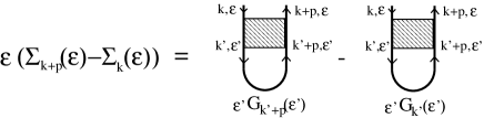
FIG. 10.: The generalized Ward identity with respect to the heat velocity.

Hereafter, we write that $k=({\epsilon},{{\bf k}},{\sigma})$. The $n$-th order skeleton diagrams for the self-energy are given by

$$\Sigma_{k}^{(n)} = \sum_{P,\{k_{i}\}}\frac{A(P)}{n!}G_{k_{1}}G_{k_{2}}\cdots G_{k_{2n-1}}$$ (D4)

$$\times U(k,k_{{\alpha}_{1}}|k_{{\alpha}_{2}},k_{{\alpha}_{3}})U(k_{{\alpha}_{4}},k_{{\alpha}_{5}}|k_{{\alpha}_{6}},k_{{\alpha}_{7}})\cdots U(k_{{\alpha}_{4n-4}},k_{{\alpha}_{4n-3}}|k_{{\alpha}_{4n-2}},k),$$

where $P$ represents the permutation of $(4n-2)$-numbers, $({\alpha}_{1},{\alpha}_{2},\cdots,{\alpha}_{4n-2})=P(1,1,2,2,\cdots,2n-1,2n-1)$. $A(P)=\pm 1$ for a skelton diagram, and $A(P)=0$ for others. $U(k_{1},k_{2}|k_{3},k_{4})$ is the two-body interaction where $k_{1},k_{3}$ are incoming and $k_{2},k_{3}$ are outgoing, respectively [27, 35]. Here we consider the on-site Coulomb interaction: $U(k_{1},k_{2}|k_{3},k_{4})=U\delta_{{{\bf k}}_{1}+{{\bf k}}_{3},{{\bf k}}_{2}+{{\bf k}}_{4}}\delta_{{\epsilon}_{1}+{\epsilon}_{3},{\epsilon}_{2}+{\epsilon}_{4}}\delta_{{\sigma}_{1},{\sigma}_{2}}\delta_{{\sigma}_{3},{\sigma}_{4}}\delta_{{\alpha}_{1},-{\sigma}_{3}}$. Note that in eq.(D4), the tadpole-type (Hartree-type) diagrams are dropped because they are $k$-independent.

Next, we consider the right-hand-site of eq.(D2), which can be rewritten as

$$T\sum_{{\epsilon}^{\prime}{{\bf k}}^{\prime}}\left[\Gamma^{I}(k;k+{{\bf p}}|k^{\prime},k^{\prime}-{{\bf p}})-\Gamma^{I}(k;k+{{\bf p}}|k^{\prime}+{{\bf p}},k^{\prime})\right]G_{{{\bf k}}^{\prime}}({\epsilon}^{\prime}){\epsilon}^{\prime},$$ (D5)

which is shown in fig.11.

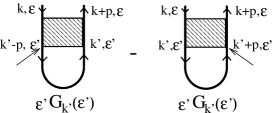
FIG. 11.:

The diagrammatic expression for eq.(D5). Here, the momentum conservation is violated by ${{\bf p}}$ only at the junction pointed by the arrow.

Then, the $n$-th order skeleton diagrams for eq.(D5) is expressed as

$$\sum_{P,\{k_{i}\}}\frac{A(P)}{n!}G_{k_{1}}G_{k_{2}}\cdots G_{k_{2n-1}}$$ (D6)

$$\ \times\biggl{\{}\ \Bigl{[}{\epsilon}_{{\alpha}_{1}}U(k,k_{{\alpha}_{1}}-{{\bf p}}|k_{{\alpha}_{2}},k_{{\alpha}_{3}})+{\epsilon}_{{\alpha}_{1}}U(k,k_{{\alpha}_{1}}|k_{{\alpha}_{2}}k_{{\alpha}_{3}}-{{\bf p}})-{\epsilon}_{{\alpha}_{2}}U(k,k_{{\alpha}_{1}}|k_{{\alpha}_{2}}+{{\bf p}},k_{{\alpha}_{3}})\Bigr{]}$$ (D7)

$$\ \ \ \ \ \ \ \ \ \ \times U(k_{{\alpha}_{4}},k_{{\alpha}_{5}}|k_{{\alpha}_{6}},k_{{\alpha}_{7}})\cdots U(k_{{\alpha}_{4n-4}},k_{{\alpha}_{4n-3}}|k_{{\alpha}_{4n-2}},k+{{\bf p}})$$ (D8)

$$\ \ \ \ \ \ +\Bigl{[}{\epsilon}_{{\alpha}_{5}}U(k_{{\alpha}_{4}},k_{{\alpha}_{5}}-{{\bf p}}|k_{{\alpha}_{6}},k_{{\alpha}_{7}})+{\epsilon}_{{\alpha}_{7}}U(k_{{\alpha}_{4}},k_{{\alpha}_{5}}|k_{{\alpha}_{6}},k_{{\alpha}_{7}}-{{\bf p}})$$ (D9)

$$\ \ \ \ \ \ \ \ \ \ \ \ -{\epsilon}_{{\alpha}_{4}}U(k_{{\alpha}_{4}}+{{\bf p}},k_{{\alpha}_{5}}|k_{{\alpha}_{6}},k_{{\alpha}_{7}})-{\epsilon}_{{\alpha}_{6}}U(k_{{\alpha}_{4}},k_{{\alpha}_{5}}|k_{{\alpha}_{6}}+{{\bf p}},k_{{\alpha}_{7}})\Bigr{]}$$ (D10)

$$\ \ \ \ \ \ \ \ \ \ \times U(k,k_{{\alpha}_{1}}|k_{{\alpha}_{2}},k_{{\alpha}_{3}})\cdots U(k_{{\alpha}_{4n-4}},k_{{\alpha}_{4n-3}}|k_{{\alpha}_{4n-2}},k+{{\bf p}})$$ (D11)

$$\ \ \ \ \ \ +\cdots$$ (D12)

$$\ \ \ \ \ \ +\Bigl{[}{\epsilon}_{{\alpha}_{4n-3}}U(k_{{\alpha}_{4n-4}},k_{{\alpha}_{4n-3}}-{{\bf p}}|k_{{\alpha}_{4n-2}},k+{{\bf p}})-{\epsilon}_{{\alpha}_{4n-4}}U(k_{{\alpha}_{4n-4}}+{{\bf p}},k_{{\alpha}_{4n-3}}|k_{{\alpha}_{4n-2}},k+{{\bf p}})$$ (D13)

$$\ \ \ \ \ \ \ \ \ \ \ \ \ \ \ -{\epsilon}_{{\alpha}_{4n-2}}U(k_{{\alpha}_{4n-4}},k_{{\alpha}_{4n-3}}|k_{{\alpha}_{4n-2}}+{{\bf p}},k+{{\bf p}})\Bigr{]}$$ (D14)

$$\ \ \ \ \ \ \ \ \ \ \times U(k,k_{{\alpha}_{1}}|k_{{\alpha}_{2}},k_{{\alpha}_{3}})\cdots U(k_{{\alpha}_{4n-8}},k_{{\alpha}_{4n-7}}|k_{{\alpha}_{4n-6}},k_{{\alpha}_{4n-5}})\ \biggr{\}}.$$ (D15)

Because of the relation $U(k_{1}+{{\bf p}},k_{2}|k_{3},k_{4})=U(k_{1},k_{2}|k_{3}+{{\bf p}},k_{4})=U(k_{1},k_{2}-{{\bf p}}|k_{3},k_{4})=U(k_{1},k_{2}|k_{3},k_{4}-{{\bf p}})$ and the energy conservation with respect to $U$, we see that eq.(D15) $+\ {\epsilon}(\Sigma_{k}-\Sigma_{k+{{\bf p}}})=0$. As a result, the generalized Ward identity, eq.(D2) is proved in the framework of the microscopic perturbation theory.

By taking the limit $|{{\bf p}}|\rightarrow 0$ of eq.(D2), we obtain

$${\epsilon}_{n}\cdot{\vec{\nabla}}_{k}\Sigma_{{{\bf k}}}({\epsilon}_{n}) = T\sum_{{\epsilon}_{n^{\prime}}{{\bf k}}^{\prime}}\lim_{{{\bf p}}\rightarrow 0}\Gamma^{I}({{\bf k}}{\epsilon}_{n};{{\bf k}}+{{\bf p}},{\epsilon}_{n}|{{\bf k}}^{\prime}+{{\bf p}},{\epsilon}_{n^{\prime}};{{\bf k}}^{\prime}{\epsilon}_{n^{\prime}})\cdot G_{{{\bf k}}^{\prime}+{{\bf p}}}({\epsilon}_{n^{\prime}})G_{{{\bf k}}^{\prime}}({\epsilon}_{n^{\prime}})$$ (D17)

$$\times{\epsilon}_{n^{\prime}}\left({\vec{v}}_{{{\bf k}}^{\prime}}^{0}+{\vec{\nabla}}_{k^{\prime}}\Sigma_{{{\bf k}}^{\prime}}({\epsilon}_{n^{\prime}})\right).$$

Equation (D17) is rewritten by using the reducible four-point vertex $\Gamma$ as

$${\epsilon}_{n}\cdot{\vec{\nabla}}_{k}\Sigma_{{{\bf k}}}({\epsilon}_{n})=T\sum_{{\epsilon}_{n^{\prime}}{{\bf k}}^{\prime}}\lim_{{{\bf p}}\rightarrow 0}\Gamma({{\bf k}}{\epsilon}_{n};{{\bf k}}+{{\bf p}},{\epsilon}_{n}|{{\bf k}}^{\prime}+{{\bf p}},{\epsilon}_{n^{\prime}};{{\bf k}}^{\prime}{\epsilon}_{n^{\prime}})\cdot G_{{{\bf k}}^{\prime}+{{\bf p}}}({\epsilon}_{n^{\prime}})G_{{{\bf k}}^{\prime}}({\epsilon}_{n^{\prime}})\cdot{\epsilon}_{n^{\prime}}{\vec{v}}_{{{\bf k}}^{\prime}}^{0}.$$ (D18)

After the analytic continuation of eq.(D18), we find that

$${\vec{\nabla}}_{k}\Sigma_{{{\bf k}}}^{\rm R}({\epsilon})\cdot{\epsilon}=\sum_{{{\bf k}}^{\prime},i=1,3}\int\frac{d{\epsilon}^{\prime}}{4\pi i}{\cal T}^{1i}({{\bf k}}{\epsilon},{{\bf k}}^{\prime}{\epsilon}^{\prime})g_{{{\bf k}}^{\prime}}^{(i)}({\epsilon}^{\prime})\cdot{\vec{v}}_{{{\bf k}}^{\prime}}^{0}{\epsilon}^{\prime},$$ (D19)

where the four-point vertex ${\cal T}^{ij}$ is introduced by Eliashberg in ref. [6], and $g_{{{\bf k}}}^{(i)}({\epsilon})$ is introduced in §II. Thus, the Ward identity, eq.(D19), is derived in terms of the diagrammatic technique. Equation (D19) is equivalent to eq.(48), which is expressed in terms of the zero temperature perturbation method.

We note that “the usual Ward identity” related to the charge conservation law is given by [26, 27]

$${\vec{\nabla}}_{k}\Sigma_{{{\bf k}}}^{\rm R}({\epsilon})=\sum_{{{\bf k}}^{\prime},i=1,3}\int\frac{d{\epsilon}^{\prime}}{4\pi i}{\cal T}^{1i}({{\bf k}}{\epsilon},{{\bf k}}^{\prime}{\epsilon}^{\prime})g_{{{\bf k}}^{\prime}}^{(i)}({\epsilon}^{\prime}){\vec{v}}_{{{\bf k}}^{\prime}}^{0}.$$ (D20)

According to eqs. (D19) and (D20),

$$\sum_{{{\bf k}}^{\prime},i=1,3}\int\frac{d{\epsilon}^{\prime}}{4\pi i}{\cal T}^{1i}({{\bf k}}{\epsilon},{{\bf k}}^{\prime}{\epsilon}^{\prime})g_{{{\bf k}}^{\prime}}^{(i)}({\epsilon}^{\prime})\cdot{\vec{v}}_{{{\bf k}}^{\prime}}^{0}{\epsilon}^{\prime}\ =\ {\epsilon}\cdot\sum_{{{\bf k}},i=1,3}\int\frac{d{\epsilon}^{\prime}}{4\pi i}{\cal T}^{1i}({{\bf k}}{\epsilon},{{\bf k}}^{\prime}{\epsilon}^{\prime})g_{{{\bf k}}^{\prime}}^{(i)}({\epsilon}^{\prime}){\vec{v}}_{{{\bf k}}^{\prime}}^{0}.$$ (D21)