Non-equilibrium Gross-Pitaevskii dynamics of boson lattice models

Abstract

Motivated by recent experiments on trapped ultra-cold bosonic atoms in an optical lattice potential, we consider the non-equilibrium dynamic properties of such bosonic systems for a number of experimentally relevant situations. When the number of bosons per lattice site is large, there is a wide parameter regime where the effective boson interactions are strong, but the ground state remains a superfluid (and not a Mott insulator): we describe the conditions under which the dynamics in this regime can be described by a discrete Gross-Pitaevskii equation. We describe the evolution of the phase coherence after the system is initially prepared in a Mott insulating state, and then allowed to evolve after a sudden change in parameters places it in a regime with a superfluid ground state. We also consider initial conditions with a “$\pi$ phase” imprint on a superfluid ground state (i.e. the initial phases of neighboring wells differ by $\pi$), and discuss the subsequent appearance of density wave order and “Schrödinger cat” states.

I Introduction

With the emerging experimental studies of ultra-cold atoms in a parabolic trap and a periodic optical lattice potential Kasevich ; Bloch (the wavelength of the optical potential is much smaller than the dimensions of the trap), new possibilities for studying the physics of interacting bosons have emerged. At equilibrium, the bosons can undergo a transition from a superfluid to an insulator as the strength of the optical potential is increased Fisher ; Sachdev ; Monien ; Elstner ; Amico ; Jaksh . However, the facile tunability and long characteristic time scales of these systems also offer an opportunity to investigate non-equilibrium dynamical regimes that have not been accessible before. In this context, there have been a few recent theoretical studies of the dynamics of bosons in a periodic potential: Ref. Stringari, computed the oscillation frequency of the center of mass of a superfluid state of bosons, while some non-equilibrium issues were addressed in papers Franzosi ; Bishop ; Bishop2 which appeared while this paper was being completed.

A description of the purpose of this paper requires an understanding of the different parameter regimes of the boson system, which we will assume is well described by the single-band Hubbard model:

$$\mathcal{H} = \sum_{j}\Biggl{[}-J(a_{j}^{\dagger}a_{j+1}+a_{j+1}^{\dagger}a_{j})+V_{j}a_{j}^{\dagger}a_{j}$$ (1)

$$~{}~{}~{}~{}~{}~{}+{U\over 2}a_{j}^{\dagger}a_{j}(a_{j}^{\dagger}a_{j}-1)\Biggr{]}.$$

Here $a_{j}$ is a canonical Bose annihilation operator on sites of the optical lattice (“wells”) labeled by the integer $j$, $J$ is the tunneling amplitude between neighboring lattice sites, $U>0$ in the repulsive interaction energy between bosons in the same lattice minimum, and $V_{j}$ is a smooth external potential which we will take to be parabolic. We will mainly consider the case of a one-dimensional optical lattice, relevant to the experiments of Ref. Kasevich, , but generalization to higher dimensions is possible. The form of $V_{j}$ and the chemical potential of the bosons determine another important parameter: $N$, the mean number of bosons at the central site (more precisely, at the site where $V_{j}$ is smallest); we shall mainly consider the case $N\gg 1$ here. A dimensionless measure of the strength of the interactions between the bosons is the coupling

$$\lambda\equiv\frac{UN}{J};$$ (2)

the different physical regimes of $\mathcal{H}$ are also conveniently dilineated by the values of $\lambda$.

When the interactions between the bosons are strong enough, $\lambda>\lambda_{SI}$, the ground state of $\mathcal{H}$ undergoes a quantum phase transition from a superfluid to a Mott insulator (see Appendix A). It is known that Fisher :

$$\lambda_{SI}\sim N^{2}.$$ (3)

So for the case where $N$ is large, there is a wide regime, $1\ll\lambda\ll N^{2}$, where the interactions between the bosons are very strong, but the ground state is nevertheless a superfluid. A description of the dynamical properties of $\mathcal{H}$ in this regime is one of central purposes of this paper.

For $N$ large, and $\lambda$ smaller than $\lambda_{SI}$, it is widely accepted Franzosi that the low temperature dynamics of $\mathcal{H}$ can be described by treating the operator $a_{j}$ as a classical $c$-number. (We will investigate the conditions for the validity of this classical approximation more carefully in Section II, where we will also discuss the time range over which it can be applied.) More precisely, we introduce the dimensionless complex dynamical variable $\psi_{j}(t)$ whose value is a measure of $\langle a_{j}(t)\rangle/\sqrt{N}$; then its dynamics is described by the classical Hamiltonian

$$H_{GP}=\sum_{j}\left[-(\psi_{j}^{\star}\psi_{j+1}+\psi_{j+1}^{\star}\psi_{j})+\frac{V_{j}}{J}|\psi_{j}|^{2}+{\lambda\over 2}|\psi_{j}|^{4}\right],$$ (4)

and the Poisson brackets

$$\left\{\psi_{j},\psi_{j}^{\star}\right\}=\delta_{ij}.$$ (5)

Here, and henceforth, we measure time in units of $\hbar/J$. The resulting equations of motion are, of course, a discrete version of the familiar Gross-Pitaevskii (GP) equations. We will often impose a parabolic confining potential, in which case

$${V_{j}\over J}={\xi\over 2}j^{2}.$$

A nonuniform potential $V_{j}$ also can lead to localization of bosons in separate wells; in particular, even without interaction ($\lambda=0$), when $|V_{j+1}-V_{j}|\geq 2J$ the eigenmodes of (4) become localized. Note that this localization is a purely semiclassical effect, described by the GP equations. If $V_{j}$ is smooth then for $\lambda>\lambda_{SI}$, the system undergoes a transition to nonuniform insulating state Troyer ; Svistunov .

Describing the non-equilibrium quantum Bose dynamics for $\lambda<\lambda_{SI}$ is now reduced to a problem of integrating the classical equations of motion implied by (4,5). However, it remains to specify the initial conditions for the classical equations; these clearly depend upon the physical situations of interest, and we shall consider here two distinct cases, which are discussed in the following subsections

I.1 Mott insulating initial state

Consider the physical situation (of current experimental interest Kasevich2 ) where for $t\leq 0$ the bosons are in a Mott insulating state with $\lambda>\lambda_{SI}$, and at time $t=0$ the optical lattice potential is suddenly reduced so that $\lambda<\lambda_{SI}$ for all $t>0$. Clearly, the GP equations should apply for $t>0$, and the Mott insulating initial state will impose initial conditions which we now describe. The required initial conditions are readily deduced by thinking about the full quantum Heisenberg equations of motion for $a_{j}(t)$ implied by $\mathcal{H}$. By integrating these equations, one can, in principle, relate any observable to the expectation values of products of powers of $a_{j}^{\dagger}(t=0)$ and $a_{j}(t=0)$. For the Mott insulator with $\lambda\gg\lambda_{SI}$ these expectation values have a very simple structure: they factorize into products of expectation values on each site, and are non-zero only if the number of creation and annihilation operators on each site are equal. Furthermore, for large $N$, we can also ignore the ordering of the $a_{j}$ and $a_{j}^{\dagger}$ operators on each site, and e.g. we obtain to leading order in $1/N$:

$$\left\langle a_{j}^{\dagger n}(t=0)a_{\ell}^{m}(t=0)\right\rangle\approx\delta_{nm}\delta_{j\ell}\left(N_{j}\right)^{n},$$ (6)

where we have accounted for a possible spatial inhomogeneity by introducing $N_{j}$ (a number of order $N$), the number of bosons at site $j$ in the Mott insulator. In terms of the classical variables $\psi_{j}$, the $t=0$ expectation values in (6) are easy to reproduce. We simply choose

$$\psi_{j}(t=0)=\sqrt{N_{j}/N}e^{i\phi_{j}}$$ (7)

where the $\phi_{j}$ are independent random variables which are uniformly distributed between $0$ and $2\pi$. In this manner, we have mapped the fully deterministic quantum time evolution of $\mathcal{H}$ to the stochastic and classical time evolution of $H_{GP}$. In practice, the procedure is then as follows: choose a large ensemble of initial values of $\phi_{j}$, and deterministically evolve $H_{GP}$ for each such initial condition; the expectation value of any quantum observable at time $t$ is then given by the average value of the corresponding classical observable at time $t$, with the average being taken over the random variables $\phi_{j}$. In particular

$$\left\langle a_{j}^{\dagger n}(t)a_{j^{\prime}}^{m}(t)\right\rangle_{Q}\approx N\left\langle\psi_{j}^{\star n}(t)\psi_{j^{\prime}}^{m}(t)\right\rangle_{\mbox{random $\phi_{\ell}$}},$$ (8)

where we have indicated that the angular brackets on the left represent a traditional quantum expectation value, while those on the right represent an average over the independent variables $\phi_{j}$ specified by (7) at time $t=0$. We will henceforth implicitly assume that all angular brackets have the meaning specified in (8), depending upon whether they contain quantum or classical variables.

An important property of (8) is that while we must have $j\,^{\prime}=j$ for a non-zero result at $t=0$, this is no longer true for $t>0$. In particular, non-zero correlations can develop for large $|j\,^{\prime}-j|$ as time evolves, corresponding to a restoration of phase coherence. Indeed the ground state for $\lambda<\lambda_{SI}$ is superfluid and thermalization must lead to increase of the phase correlations. However, in this paper we show, that even without relaxation the coherence can be restored dynamically. (Of course, as we are looking at one dimensional systems and the final state is expected to be thermalized at a non-zero temperature, the phase correlations cannot be truly long-range and must decay exponentially at large enough scales: however, guided by the experimental situation, we will look at relatively small systems for which this is not an issue.) Describing the dynamics of the restoration of this phase coherence is also a central purpose of this paper. We shall characterize the phase coherence by studying the expectation value of

$$\mathcal{D}_{g}(t)=\frac{1}{M}\sum_{j\neq\ell}g(|j-\ell|)\left\langle\psi_{j}^{\star}(t)\psi_{\ell}(t)\right\rangle$$ (9)

where $M$ is the number of lattice sites (for a nonuniform external potential $V_{j}$, $M$ is just the ratio of the total number of bosons to the number of bosons in central well), and $g$ is some suitably chosen weight function. Observables closely related to $\mathcal{D}_{g}$ are measured upon detecting the atoms after releasing the trap. At time $t=0$, $\mathcal{D}_{g}(0)=0$, and we will be interested in the deviations of $\mathcal{D}_{g}(t)$ from this value for $t>0$, an increase corresponding to an enhancement of superfluid phase coherence. We note, in passing, that a closely related procedure was used earlier Kedar to describe the onset of phase coherence after a sudden quench from high temperature; here, we are always at zero temperature, and move into a superfluid parameter regime by a sudden change in the value of $\lambda$.

We will begin our analysis of the structure of $\mathcal{D}_{g}(t)$ by considering the case with two wells ($M=2$) in Section II.1. For the weakly interacting case ($\lambda\ll 1$), $\mathcal{D}_{g}(t)$ exhibits Josephson oscillations with a period of order unity; the weak interactions lead to a decay of oscillations with a slow ($t^{-1/2}$) saturation of the coherence at a steady-state value at a time scale $t\propto\lambda^{-1}$. For $\lambda\gg 1$ the oscillations are suppressed and $\mathcal{D}_{g}(t)$ saturates at $t\propto 1/\sqrt{\lambda}$, which is, in fact, shorter than a single tunneling time. For this two lattice site case we can also obtain a complete solution for $\mathcal{D}_{g}(t)$ for the quantum Hamiltonian $\mathcal{H}$ (described in Section II.1.2), and this allows a detailed analysis on the regime of validity of the semiclassical GP equations. We show that the semiclassical approach is valid for two lattice sites when $N$ is large and $t<N/\lambda$. This is, in fact, a general result which implies that the quantum mechanics becomes important when time exceeds inverse energy level spacing. For more than two lattice sites, the energy splitting scales as the inverse of the total number of particles and at $\lambda\ll 1$, the semiclassical conditions are virtually always fulfilled. It is surprising that even with a small number of particles $N=4$, and weak interactions, the GP equations give an excellent description of the system evolution, apart from overall numerical prefactor $(1+2/N)$, which is not small in this case.

The restoration of coherence is also studied in the many well case in Section III.1. We discuss the case without an external potential in Section III.1.1; with an equal number of particles initially in all the wells, phase correlations develop only in the interacting case ($\lambda>0$). This is true for both periodic and open boundary conditions. Similar to the two well case, in the weakly interacting regime phase correlations will oscillate in time. However these oscillations will be periodic only for particular number of wells: $M=2,3,4,6$ for periodic boundary conditions and $M=2,3,5$ for open boundary conditions. For other numbers of wells, the oscillations are chaotic. As for the two well case, a stronger interaction results in decay of correlations in time, leading to the steady state.

Next, in Section III.1.2, we consider the restoration of phase coherence for the experimentally important case of a parabolic potential. The results are quite different for this case, and phase correlations develop even without interactions. In a weak parabolic potential, $\mathcal{D}_{g}(t)$ oscillates with a frequency which scales as the square root of the parabolicity, $\xi$. This frequency is closely related to the oscillation frequency discussed recently by Kramer et al. Stringari for the case where the center of mass of the atomic gas is displaced. In the present situation, there is no displacement of the center of mass, but the same oscillation is excited upon a sudden change in the value of $\lambda$. The oscillations decay even at $\lambda=0$; weak or intermediate interactions $\lambda\leq 1$ do not change the noninteracting picture much. The amplitude of the oscillations become more pronounced for $\lambda\approx 1$, but for $\lambda\gg 1$ the oscillations are suppressed as for the flat potential.

While this work was being completed, we became aware of related results of Altman and Auerbach also addressing the restoration of phase coherence in a Mott insulator. However, there are some significant differences in the physical situations being addressed. Above, we have considered a system deep in the Mott insulating phase (with $\lambda\gg\lambda_{SI}$) taken suddenly to parameters for which the ground state was deep in the superfluid phase (with $\lambda\ll\lambda_{SI}$). In contrast, Ref. aa, consider the case when both the initial and final values of $\lambda$ were not too far from $\lambda_{SI}$, but remained on opposite sides of it. For $\lambda$ close to $\lambda_{SI}$, and at temperatures not too small, a “relativistic Gross-Pitaevski” equation had been proposed in Ref. ssrelax, as a description of the “Bose molasses” dynamics of the order parameter. The conditions under which oscillations in the amplitude of the order parameter would be underdamped were also presentedssrelax . Altman and Auerbach aa advocated that the same equations could describe the time evolution of the amplitude of the order parameter as it evolved from the Mott insulator (with zero amplitude) to the superfluid (with finite amplitude) at zero temperature. We review issues related to the damping of the amplitude mode in Appendix B. Altman and Auerbach aa also considered the situation without an external potential ($V_{j}\equiv 0$). We have noted above that such a potential changed our results significantly; in Appendix A we discuss the significant role of the external potential in the equilibrium properties for $\lambda\approx\lambda_{SI}$.

I.2 Modulated phase initial state

A second set of initial conditions we consider is the case in which the parameter values always correspond to a superfluid ground state i.e. $\lambda<\lambda_{SI}$. For time $t\leq 0$ we imagine that $\lambda$ takes some fixed value and the phases $\phi_{j}$ have some known set of fixed, non-random values at $t=0$ and we follow the subsequent evolution of the bosons using the discrete GP equation. The phase imprint can be experimentally achieved by e.g. applying a short (compared to a single tunneling time) pulse of external field to the condensate. A case of special interest will be when there is a relative $\pi$ phase shift between neighboring wells:

$$\phi_{j}=j\pi.$$ (10)

For two wells with equal $N_{j}$ and relatively small $\lambda$, this state is metastable (this is also the case for even $M$ and periodic boundary conditions). However, if the interaction $\lambda$ becomes larger than a critical value, this equilibrium becomes unstable and the bosons spontaneously form a “dipole” state Franzosi ; Vardi ; Raghavan in which most of them occupy one of the two wells (see Section II.2). Upon accounting for quantum tunneling in a system with a finite number of bosons, the state obtained is a superposition of the two dipole states restoring translational symmetry. However, in case of infinite number of wells (see Section III.2) the tunneling between the two dipole configurations is negligible and translational symmetry is broken by the appearance of a density wave of bosons with a period of two lattice spacings. This effect is similar to that studied in Ref. Sachdev1, for the case of a Mott insulator in a strong electric field.

Related to this instability is a very interesting possibility of forming a Schrödinger cat state Kasevich1 . We show in Section III.2 that if the system is initially in the “$\pi$ state”, and the interaction is slowly increased, then at certain point all the bosons spontaneously move into one of the wells. If quantum mechanical corrections are taken into account then the final configuration is the superposition of the states with all bosons in one of the wells. This effect opens the possibility of dynamical forming of a strongly entangled state of bosons.

II Semiclassical versus quantum dynamics of two coupled interacting Bose systems

The comparison between the semiclassical and quantum theory of the two-well system has been presented earlier by Milburn et al. milburn , although for initial conditions different from those we shall consider here.

First we will focus on the semiclassical description of the two well system, when the total number of bosons is much greater than 1. In this case the Gross-Pitaevskii equations implied by (4) and (5) are

$$i{\partial\psi_{1}\over\partial t}=-\psi_{2}+\lambda|\psi_{1}|^{2}\psi_{1},$$ (11)

$$i{\partial\psi_{2}\over\partial t}=-\psi_{1}+\lambda|\psi_{2}|^{2}\psi_{2},$$ (12)

The total number of bosons $|\psi_{1}|^{2}+|\psi_{2}|^{2}$ is a constant of the motion; with our normalization for $\psi_{j}$ described above (4), we have $|\psi_{1}|^{2}+|\psi_{2}|^{2}=2$.

We use the parameterization:

$$\psi_{1,2}=\sqrt{1\mp n}{\rm e^{i\theta\mp i\phi/2}}.$$ (13)

Note that only the relative phase of $\psi_{1}$ and $\psi_{2}$ is an observable. Substituting (13) into (11) and (12) we obtain:

$${d^{2}n\over dt^{2}}+4n+4\lambda n\sqrt{1-n^{2}}\cos\phi=0,$$ (14)

$${d\cos\phi\over dn}={n\over 1-n^{2}}\cos\phi+{\lambda n\over{\sqrt{1-n^{2}}}}.$$ (15)

After further manipulation this system reduces to a single second order differential equation for the continuous variable $n$:

$${d^{2}n\over dt^{2}}+4n+4\lambda n\left(\cos\phi_{0}+{\lambda n^{2}\over 2}\right)=0$$ (16)

with initial conditions: $n(0)=n_{0}$, $dn(0)/dt=2\sin{\phi_{0}}$. Similar equations were derived in Franzosi ; Raghavan . Without interaction ($\lambda=0$) we have a situation of a single Josephson junction described by a free harmonic oscillator. The interaction $\lambda$ is responsible for the anharmonicity. Note that for $\lambda\leq 1$ the solutions $n=0$, $\phi=0,\pi$ are stationary; i.e. the phase difference between the two wells can be either $0$ or $\pi$. On the other hand for $\lambda>1$ the solution with $\phi=\pi$ becomes unstable Franzosi ; Raghavan , and instead the new minima appear at

$$n_{\rm min}=\pm\sqrt{2(\lambda-1)\over\lambda^{2}}.$$ (17)

We will now consider the properties of the two well system for the two classes of initial conditions discussed in Section I in turn. Each subsection below also contains a comparison with the exact results obtained by a full quantum solution of $\mathcal{H}$.

II.1 Mott insulating initial state

As in Section I.1, let us assume that initially the two condensates are completely uncoupled. We will consider their evolution in the semiclassical and quantum calculations in turn:

II.1.1 Semiclassical theory

¿From the discussion in Section I.1, we have $n_{0}=0$ and $\phi_{0}$ is a uniform random variable. We will study the correlation between $\psi_{1}$ and $\psi_{2}$ as a function of time. It is easy to show that

$$\langle\psi_{2}^{\star}(t)\psi_{1}(t)+\psi_{1}^{\star}(t)\psi_{2}(t)\rangle={\lambda\over 4}\langle n^{2}(t)\rangle,$$ (18)

where the average is taken over all possible initial phases $\phi_{0}$. The correlator is proportional to the product of the coupling constant $\lambda$ and the variance of $n$, reflecting the usual phase-number uncertainty relation.

Before proceeding with quantitative analysis let us argue qualitatively what happens with the system. Suppose $\lambda\ll 1$. Then (16) is equivalent to the motion of a particle in a harmonic potential with random initial velocity. Because the frequency of the harmonic oscillator doesn’t depend on the amplitude, $\langle n^{2}(t)\rangle$ is a periodic function of time with $T=\pi/2$. If $\lambda$ is still small but not negligible, then (16) still describes motion in a harmonic potential, which, however, depends on the initial conditions. As a result the oscillations of $\langle n^{2}(t)\rangle$ become quasiperiodic and decay with time. In the limit of large $\lambda$ the oscillations completely disappear and the steady state solution develops during the time $t\sim 1/\sqrt{\lambda}$.

For weak coupling $\lambda$, equation (16) can be solved explicitly. Thus for $\lambda=0$

$$\langle n^{2}(t)\rangle={1-\cos 4t\over 4}.$$ (19)

For small $\lambda$ the approximate analytical solution is:

$$\langle n^{2}(t)\rangle\approx{1\over 4}-{1\over 2\pi}\int\limits_{0}^{\pi}\sin^{2}\phi_{0}\cos\left(4t\sqrt{1+\lambda\cos\phi_{0}}\right)d\phi_{0}.$$ (20)

It is easy to see that at large $t$ we have the following asymptotic behavior:

$$\langle n^{2}(t)\rangle\approx{1\over 4}-{1\over\sqrt{16\pi\lambda t}}\left[\cos\left(4t\sqrt{1+\lambda}+{\pi\over 4}\right)\right.$$

$$\left.+\cos\left(4t\sqrt{1-\lambda}-{\pi\over 4}\right)\right],$$ (21)

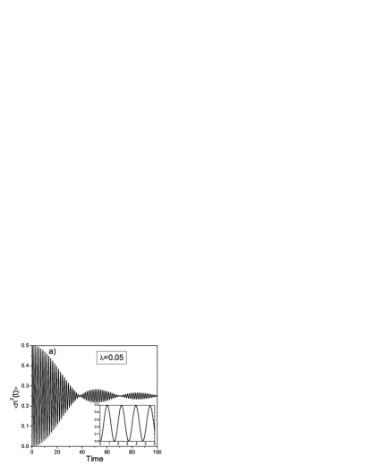
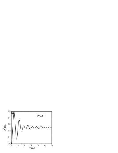
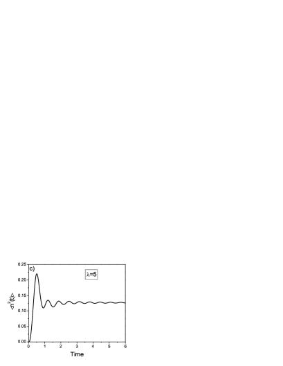
Figure 1: Semiclassical variance of $n$ as a function of time. The insert on the top graph has a different time scale.

so that the variance of $n$ approaches the steady state value of one fourth. We note that the amplitude of oscillations decays with time as $t^{-1/2}$ and on top of that there are beats with the characteristic frequency $\omega_{beats}\approx 4\lambda$ (see Fig. 1). For large $\lambda$ the oscillations decay very rapidly and $\langle n^{2}(t)\rangle$ quickly saturates at the steady state value, which decreases with $\lambda$ (see Fig.1).

II.1.2 Quantum theory

Let us now study the quantum case. The Heisenberg equations of motion are:

$${d\hat{a}_{j}\over dt}=i\,[{\cal H},\hat{a}_{j}],$$ (22)

where square brackets denote commutator, $j=1,2$ and the Hamiltonian ${\cal H}$ is given by (1). It turns to be convenient to use the following Heisenberg operators:

$$\left\{\begin{array}[]{l}\hat{\Phi}=\hat{a}_{2}^{\dagger}\hat{a}_{1}-\hat{a}_{1}^{\dagger}\hat{a}_{2},\\ \hat{\Psi}=\hat{a}_{2}^{\dagger}\hat{a}_{1}+\hat{a}_{1}^{\dagger}\hat{a}_{2},\\ \hat{n}=\hat{a}_{2}^{\dagger}\hat{a}_{2}-\hat{a}_{1}^{\dagger}\hat{a}_{1}.\end{array}\right.$$ (23)

We introduce hats over the operators to distinguish them from numbers appearing in the semiclassical treatment and expectation values of the operators . It is easy to see that the following combination

$$\hat{\Psi}-{\lambda\over 2N}\hat{n}^{2}\equiv\hat{\Psi}-{U\over 4J}\hat{n}^{2}$$ (24)

commutes with the Hamiltonian. Using this fact the system (22) can be reduced to a single differential equation:

$${d^{2}\hat{n}\over dt^{2}}+4\hat{n}+{2\lambda\over N}\left\{\hat{n},\hat{\Psi}_{s}\right\}_{+}+{\lambda^{2}\over N^{2}}(2\hat{n}^{3}-\left\{\hat{n},\hat{n}_{s}^{2}\right\}_{+})=0$$ (25)

with the initial conditions:

$$\hat{n}(0)=\hat{n}_{s},\quad\left.{d\hat{n}\over dt}\right|_{t=0}=-2i\hat{\Phi}_{s}.$$ (26)

In the equations above $\left\{\dots\right\}_{+}$ denotes the anticommutator, and the subindex $s$ means time-independent Schrödinger operators. We note that the second relation in (26) holds for all times if we use $\hat{\Phi}$ instead of $\hat{\Phi}_{s}$.

In the noninteracting case ($\lambda=0$) the solution of (25) is:

$$\hat{n}(t)=\hat{n}_{s}\cos 2t-i\hat{\Phi}_{s}\sin 2t.$$ (27)

The initial conditions corresponding to the ground state for $\lambda\gg\lambda_{SI}$ is $|I\rangle\equiv|N/2,N/2\rangle$. Note that such a state is possible only if $N$ is even. The generalization for $N$ odd is straightforward, but we will not do it here, since our major goal is to compare quantum and semiclassical pictures. Simple computation shows that

$${n^{2}(t)\over N^{2}}\equiv{1\over N^{2}}\langle I|\hat{n}^{2}(t)|I\rangle={1-\cos 4t\over 4}{N+2\over N}.$$ (28)

Comparing (28) and (19) we see that the only difference between the semiclassical and quantum results in the noninteracting case is the presence of an extra numerical factor $1+2/N$ in (28).

In the weakly interacting regime ($\lambda\ll 1$) we can neglect terms proportional to $\lambda^{2}$. Then (25) simplifies to:

$${d^{2}\hat{n}\over dt^{2}}+4\hat{n}+{2\lambda\over N}\left\{\hat{n},\hat{\Psi}_{s}\right\}_{+}=0.$$ (29)

It is very convenient to solve this equation in the eigenbasis of $\hat{\Psi}_{s}$:

$$|k\rangle={2^{-N/2}\over\sqrt{k!(N-k)!}}(\hat{a}_{1s}^{\dagger}+\hat{a}_{2s}^{\dagger})^{k}(\hat{a}_{1s}^{\dagger}-\hat{a}_{2s}^{\dagger})^{N-k}|0\rangle,$$ (30)

where $k=0,1,\dots N$. One can show that for the initial Fock state $|I\rangle=|N/2,N/2\rangle$ the variance of $n$ is:

$${n^{2}(t)\over N(N+2)}={1\over 4}-{2^{2-N/2}\over N(N+2)}\sum\limits_{k=0}^{N/2-1}{(N\!-\!2k\!-\!1)!!\,(2k\!+\!1)!!\over(N/2-k-1)!\,k!}\cos 2t\!\left[\sqrt{1\!-\!{\lambda\over N}(4k\!+\!3\!-\!N)}\!+\!\sqrt{1\!-\!{\lambda\over N}(4k\!+\!1\!-\!N)}\right].$$ (31)

Figure 2: (a) Semiclassical (solid line) and quantum variance of $n$ as a function of time for the weak coupling case $\lambda=0.05$. Dash line corresponds to the total number of particles $N=2$, dot line does to $N=4$. Solid and dot line are indistinguishable on this plot. (b) Amplitude of the oscillations of the variance of $n$ versus time.

Comparing (31) and (21) we see that in contrast to the continuous integral in the semiclassical case there is a discrete sum in the quantum. One can formally obtain (21) from (31) in the limit $N\to\infty$ using Stirling’s formula and transforming the summation over $k$ to integration. It turns out to be more convenient to normalize the variance of $n$ to $N(N+2)$ instead of $N^{2}$. If the total number of particles $N=2$, there is only one term in (31), so the oscillations are completely undamped. For $N=4$, there are two terms and we expect perfect beats; i.e. the amplitude of oscillations first goes to zero then completely restores and so on. For $N\geq 6$ there are several terms contributing to the sum. At relatively small time scale $\lambda^{2}t/N\ll 1$ frequencies in different terms are approximately equidistant: $\Delta\Omega\approx 8\lambda/N$ so the amplitude of oscillations is a periodic function. However at a larger time scale the phases become random and periodicity disappears. Figure 2(a) shows the comparison of the variance of $n$ for $N=2$ and $N=4$ with the semiclassical result. On short time scales already $N=4$ gives an excellent agreement. In fact the semiclassical and the quantum curve (for $N=4$) are completely indistinguishable. The behavior of the amplitude of oscillations of $n^{2}$ is plotted in Fig. 2(b). It is clear that with increasing $N$, the semiclassical approximation works for longer and longer time scales (see also Ref. milburn, ). However in a quantum system the recurrence time is always finite, so ultimately at $t>1/\Delta\Omega$, the semiclassical description breaks down.

Figure 3: Variance of n as a function of time for intermediate (a) and large (b) coupling constants. Note that for larger N semiclassical approximation works well for longer time scale, but eventually always breaks down.

In Fig. 3 we present the numerical solution for the case of intermediate and strong couplings. As was discussed before for small $N$, the amplitude of oscillations fluctuates, being completely chaotic at large time scales. However, at sufficiently small time, the oscillations gradually decay, approaching the semiclassical result. At intermediate times the amplitude of the oscillations experiences beats (compare with Fig. 2). Note that for the large coupling, the semiclassical description breaks down very early.

II.2 Modulated phase initial state

We turn next to the initial conditions described in Section I.2, where the initial state has a phase order. In semiclassical picture $n$ and $\phi$ are commuting variables and we can fix them at $t=0$ independently. For simplicity let us consider $n_{0}=0$. Then from (16) it is obvious that only $\phi_{0}=0,\pi$ give the stationary solutions. As we discussed above, $n=0$ and $\phi=0$ is automatically a ground state for all positive values of interaction $\lambda$, therefore it is always stable under small fluctuations. On the other hand if $\phi_{0}=\pi$ then $n=0$ is (meta)stable for $\lambda\leq 1$ and unstable for $\lambda>1$ (see Ref. Franzosi, for the details). Suppose that we start from $\phi=\pi$, $n=0$, $\lambda=0$ and adiabatically increase $\lambda$. Then $n^{2}$ remains close to zero while $\lambda$ remains smaller than critical value. After that $n^{2}$ rapidly increases and the system spontaneously goes to the Schrödinger cat state, where all the bosons are either in the left or in the right well. A similar picture holds in the quantum mechanical description. The principal difference is that instead of a sharp transition at $\lambda=\lambda_{c}$, there is a smooth crossover between the initial and the final states. Fig. 4 shows the variance of $n$ as a function of time. For comparison we consider both symmetric ($\phi=0$) and antisymmetric ($\phi=\pi$) initial conditions.

Figure 4: Variance of $n$ for the two wells for adiabatically increasing interaction $\lambda(t)$. The initial state is (a) antisymmetric ($\phi=\pi$) and (b) symmetric ($\phi=0$).

III Semiclassical Description of Multi-well Bose Gases

The full quantum solution of the many well case rapidly becomes numerically prohibitive with increasing $N$, and so we will confine our discussion in this section to the semiclassical GP equation. From (4) and (5) this is

$$i{\partial\psi_{j}\over\partial t}=-(\psi_{j+1}+\psi_{j-1})+\frac{V_{j}}{J}\psi_{j}+\lambda|\psi_{j}|^{2}\psi_{j},$$ (32)

The equilibrium number of bosons in the central well ($j=0$) is $N$, and so $|\psi_{0}|^{2}=1$ in the Mott insulating ground state.

We divide our discussion according to the initial conditions considered in Section I.

III.1 Mott insulating initial state

We will compute the correlation function $\mathcal{D}_{g}(t)$ defined in (9) for two limiting possibilities for the weight function $g$: $g(j)=\delta_{j,1}$ and $g(j)=\,{\rm const}$, where in the former (latter) case one computes the nearest neighbor (global) phase correlation. Using the GP equations (32) we can show that

$${d\mathcal{D}_{g}(t)\over dt}= i\sum_{j\neq\ell}\left(V_{j}+\lambda|\psi_{j}(t)|^{2}\right)g(|j-\ell|)$$ (33)

$$\times\left(\psi_{j}^{\star}(t)\psi_{\ell}(t)-\psi_{\ell}^{\star}(t)\psi_{j}(t)\right).$$

Note that for uniform potential $\mathcal{D}_{g}(t)$ changes only due to the interaction. In this case, the ratio ${\cal D}_{g}(t)/\lambda$ has a finite limit at $\lambda\to 0$. We will consider the solution for $\mathcal{D}_{g}(t)$ with and without an external potential in the following subsections.

III.1.1 No external potential and periodic boundary conditions

Let us assume that the lattice forms a periodic array of quantum wells and there is no external potential ($V_{j}\equiv~{}0$). For the nearest neighbor correlation similarly to the two well case it is easy to show that

$${\cal D}_{g}(t)\equiv\sum_{j}\psi_{j}^{\star}\psi_{j+1}+\psi_{j+1}^{\star}\psi_{j}={\lambda\over 2}\sum_{j}(|\psi_{j}|^{2}-1)^{2}.$$ (34)

This equation shows that the nearest neighbor coherence is proportional to the product of the coupling constant and sum of the variances of number of bosons in each well. From the previous section we can expect that if the interaction is weak, then variances of $n_{j}$ at short time scales will be fluctuating and governed by the noninteracting tunnelling Hamiltonian. With increasing time the interaction will suppress the fluctuations leading to some steady state. In the noninteracting case, (32) is just an ordinary Schrödinger equation. with eigenstates

$$\psi_{k}(j)={1\over\sqrt{M}}\,{\rm e}^{2\pi ikj/N},$$ (35)

corresponding to the eigenenergies

$$E_{k}=-2\cos{2\pi k\over M}.$$ (36)

Here $M$ is the number of wells. Expanding the initial insulating state in terms of the eigenstates defined above and propagating them in time we obtain

$$\sum\limits_{j=1}^{N}(|\psi_{j}(t)|^{2}-1)^{2}=M\left(1-\sum_{j}|F(j,t)|^{4}\right),$$ (37)

where

$$F(j,t)={1\over M}\sum\limits_{k=0}^{N-1}{\rm e}^{2i\left(\pi kj/M+t\cos 2\pi k/M\right)}.$$ (38)

For several different values of $M$ the function ${\cal D}_{g}^{\,M}(t)$ at vanishing $\lambda$ is:

$${\cal D}_{g}^{\,2}(t)={\lambda\over 2}\sin^{2}2t,$$ (39)

$${\cal D}_{g}^{\,3}(t)={8\lambda\over 9}(2+\cos 3t)\sin^{2}{3\over 2}t,$$ (40)

$${\cal D}_{g}^{\,4}(t)={\lambda\over 4}(7+\cos 2t)\sin^{2}2t,$$ (41)

$${\cal D}_{g}^{\,5}(t)={4\lambda\over 25}(10-2\cos\sqrt{5}t-\cos\sqrt{5}t-2\cos{5\over 2}t\,\cos{3\sqrt{5}\over 2}\cos\sqrt{5}t),$$ (42)

$${\cal D}_{g}^{\,6}(t)={\lambda\over 36}(63-8\cos t-12\cos 2t-24\cos 3t-6\cos 4t-12\cos 6t-\cos 8t),$$ (43)

$${\cal D}_{g}^{\,M}(t)\to{M\lambda\over 2}\left(1-J_{0}(t)^{4}-2\sum_{m=1}^{\infty}J_{m}(t)^{4}\right)\quad\mbox{at}\quad M\to\infty.$$ (44)

Clearly ${\cal D}_{g}^{\,M}(t)$ is a periodic function only for $M=2,3,4,6$ (this is, in fact true, not only for the nearest neighbor case). For many wells the number of harmonics contributing to the variance of $n$ becomes large and oscillations become more chaotic and weaker in amplitude. In the limit $M\to\infty$, ${\cal D}_{g}^{\,M}(t)$ is a monotonically increasing function. If we add the interaction, then the overall picture remains similar to the two well case. Namely, for small $\lambda$ the amplitude of oscillations slowly decays in time. For strong interaction, the variance of $n$ reaches steady state value in a very short time scale.

In the opposite to nearest neighbors limit $g(|j-\ell|)={\,\rm const}$, one can show that at $\lambda\to 0$

$${\cal D}_{g}^{\,M}(t)\to{2\lambda\over M}\sum_{k\neq m=0}^{N-1}{\sin^{2}t\left(1+\cos(2\pi k/M)-\cos(2\pi m/M)-\cos(2\pi(k-m)/M)\right)\over 1+\cos(2\pi k/M)-\cos(2\pi m/M)-\cos(2\pi(k-m)/M)}.$$ (45)

For example

$${\cal D}_{g}^{\,2}(t)={\lambda\over 2}\sin^{2}2t,$$ (46)

$${\cal D}_{g}^{\,3}(t)={\lambda\over 45}(3-2\cos 3t-\cos 6t),$$ (47)

$${\cal D}_{g}^{\,4}(t)={\lambda\over 160}(13-12\cos 4t-\cos 8t),$$ (48)

$${\cal D}_{g}^{\,6}(t)=\lambda{1\over 240}(33+16\cos t-24\cos 2t-8\cos 6t-\cos 8t),$$ (49)

$${\cal D}_{g}^{\,M}(t)\to{M\lambda\over 2\pi^{2}}\int_{0}^{2\pi}\int_{0}^{2\pi}d\theta_{1}d\theta_{2}{\sin^{2}t(1+\cos\theta_{1}-\cos\theta_{2}-\cos(\theta_{1}-\theta_{2}))\over 1+\cos\theta_{1}-\cos\theta_{2}-\cos(\theta_{1}-\theta_{2})}\quad\mbox{at}\quad M\to\infty.$$ (50)

The behavior of ${\cal D}_{g}(t)$ at large $M$ is very different for nearest neighbor and global correlations (see Fig. 5). While the former rapidly reaches a steady state value, the latter oscillates in time. Indeed the denominator in (45) selects only low frequency harmonics in ${\cal D}_{g}$, freezing out high frequency oscillations, especially at longer time scales.

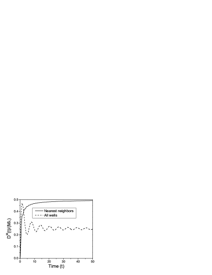
Figure 5: Time dependence of the coherence ${\cal D}_{g}(t)$ for the weakly interacting Bose gases at large number of wells ($M\to\infty$). Note that nearest neighbor correlation rapidly saturates, while the global coherence exhibits oscillations.

Figure 6: Time dependence of ${\cal D}_{g}(t)$ for 6 wells; solid and dash lines correspond to nearest neighbor and global correlations respectively. Without interaction ($\lambda\to 0$) ${\cal D}_{g}(t)$ shows regular periodic behavior in time. Nonzero interactions leads to decay of oscillations. High frequency oscillations of global correlation function are effectively suppressed.

Figure 7: Same as in Figure (6) but for 12 wells. Without interaction oscillations are chaotic. Low frequency dominate the global correlation function here as well.

Figs. 6 and 7 show ${\cal D}_{g}(t)$ for six and twelve wells respectively. Six wells give periodic time dependence, while $N=12$ corresponds to chaotic behavior. Note that in all cases high frequency modes are suppressed for the case of global phase correlations.

III.1.2 Parabolic confining potential

So far, we have considered the rather hypothetical situation of quantum wells sitting on a ring. However, usually one achieves confinement using a trap, which is equivalent to a nonuniform external potential $V_{j}$ in (32). The most common shape of this potential is parabolic ($V_{j}\propto j^{2}$) and we focus on this case, although the analysis of other potentials is similar and straightforward. As before, we will first study the non-interacting system: ($\lambda=0$).

$$i{d\psi_{j}\over dt}=-(\psi_{j+1}+\psi_{j-1})+{\xi j^{2}\over 2}\psi_{j}.$$ (51)

This is a linear Schrödinger equation with stationary states found from

$$E\psi_{j}=-(\psi_{j+1}+\psi_{j-1})+{\xi j^{2}\over 2}\psi_{j}.$$ (52)

In the Fourier space the same equation looks more familiar:

$$E\psi(k)=-2\cos k\,\psi(k)-{\xi\over 2}{d^{2}\psi(k)\over dk^{2}},$$ (53)

describing the motion of an one-dimensional particle of mass $\xi^{-1}$ living on a circle with the external potential $U(k)=-2\cos(k)$. Note that the same type of equation describes Josephson junctions with charging energy. If the parabolicity is weak ($\xi\ll 1$), then the bosons form closely spaced extended states at low energies. In the Fourier space this is equivalent to having a heavy particle in the $-2\cos k$ potential. With a good accuracy one can describe the energy spectrum inside such a well using the WKB approximation. This is justified both for low energies, where $-2\cos k\approx-2+k^{2}$ and the WKB gives the exact energy spectrum and for high energies WKB works well for any potential. In fact there is a little subtlety near energy close to $2$, since the potential there is almost flat and can not be approximated by a linear function, but this is not very important. So the approximate WKB spectrum is given by

$$\int_{-\pi+\cos^{-1}E/2}^{\pi-\cos^{-1}E/2}\sqrt{{2\over\xi}(E+2\cos k)}\,dk=\pi(n+1/2)$$

$$\int_{-\pi}^{\pi}\sqrt{{2\over\xi}(E+2\cos k)}\,dk=2\pi n,$$ (54)

where the top (bottom) equation corresponds to $E<2$ ($E>2$). In the first equation even or odd $n$ describes even and odd states (in both real and reciprocal space), respectively. For energies $E>2$, the second equation gives complete degeneracy between even and odd energy levels. In real space roughly all states with $E>2$ are localized in individual wells, and degenerate while those with $E<2$ are spread through many wells. Fig. 8(a) briefly summarizes this discussion showing the exact spectrum for $\xi=0.1$ (The WKB result is indistinguishable by eye from this graph).

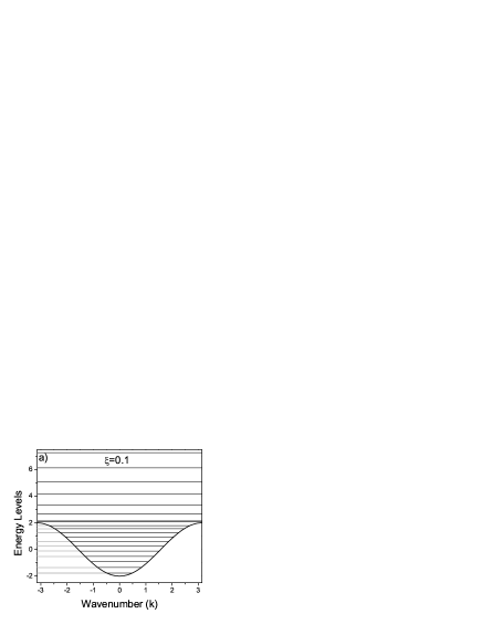
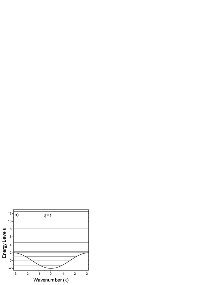
Figure 8: Energy spectrum of coupled noninteracting Bose gases in a weak (a) and intermediate (b) parabolic potential.

Clearly the low energy levels are approximately equally spaced, revealing the famous property of a harmonic potential, the spacing decreases as the energy approaches $2$, and starts linearly increasing for $E>2$ as in a usual square well. If $\xi\geq 1$ then bosons become localized within individual wells and their energies follow external potential. The crossover from weak to strong parabolicity is a finite system analog of the Anderson transition. It is important to note that this is a purely semiclassical transition in this case, because it is derived in the Gross-Pitaevskii picture. The “quantum mechanics” here originates from the wave nature of the classical field $\psi$. If the average number of bosons per well is much larger than one, then the semiclassical picture, where number of bosons and their phase commute, holds until the typical fluctuations of $\psi^{2}$ becomes of the order of $1/N\ll 1$. This occurs deep inside the insulating regime, where the energy in GP approach is anyway almost phase independent.

After deriving the energy spectrum we can proceed with study of the dynamics of the condensate. Note that (33) yields that time derivative of ${\cal D}_{g}(t)$ is not equal to zero even without interaction ($\lambda=0$). Therefore we anticipate that the results for the parabolic and flat potentials will be strongly different, at least in the weakly interacting regime. If the initial phases are uncorrelated then it is not hard to show that at $\lambda=0$

$${\cal D}_{g}(t)=2\sum_{j\neq\ell}V(j)g(|j-\ell|)\sum_{p,\alpha,\beta}N_{0}^{p}\psi_{\alpha}^{\star}(j)\psi_{\alpha}(p)\psi_{\beta}^{\star}(p)\psi_{\beta}(\ell){\sin^{2}{E_{\beta}-E_{\alpha}\over 2}t\over E_{\beta}-E_{\alpha}},$$ (55)

where $N_{0}^{p}$ is the initial number of Bosons in the well number $p$, $\psi_{\alpha}$ and $E_{\alpha}$ are the eigenfunction and energy of the level $\alpha$ respectively . If starting from the ground insulating state then

$$N_{0}^{p}=1-{V_{p}\over\mu}\quad\mbox{for}\quad V_{p}<\mu,$$ (56)

$$N_{0}^{p}=0\quad\mbox{for}\quad V_{p}>\mu,$$ (57)

with $\mu$ being a chemical potential. Let us make few comments about (55). Levels $\beta$ and $\alpha$ must have the same parity, meaning the lowest harmonic contributing to the sum will be $\omega_{\rm min}=2\,\mbox{min}_{\alpha}\,(E_{\alpha+2}-E_{\alpha})>0$. Because $N_{0}^{p}$ is centered near the bottom of the well, only levels with delocalized wavefunctions will contribute to the sum. In particular, degenerate levels with $E>2$ can be safely thrown away. If $g(|j-\ell|)$ is constant, then summation over $m$ ensures that the major contribution comes from $\beta=0$; therefore ${\cal D}_{g}(t)$ contains mostly harmonics with $\omega=E_{2}-E_{0}$, $\omega=E_{4}-E_{0}$, etc., with the strongest weight at the smallest frequency. Note that at small energies and weak parabolicity the lowest energy levels are approximately equally spaced, therefore the whole expression for ${\cal D}_{g}(t)$ will be a quasi-periodic function of a frequency $\omega\approx E_{2}-E_{0}$. However, because this equidistance is not exact, the periodicity will be only approximate, and at a short time scale the amplitude of oscillations will slowly decay. On the contrary for the nearest neighbor phase coherence $g(|j-\ell|)=\delta_{j,\ell\pm 1}$ neither $\beta$ nor $\alpha$ are bounded to the ground state and we expect that all kinds of allowed frequencies $E_{\alpha}-E_{\beta}$ will give contributions. Clearly in this case dephasing occurs much earlier and the amplitude of oscillations is much weaker. Also the characteristic frequency of the oscillations for the nearest neighbor case will be somewhat larger than that for the global case since the level separation decreases with energy. Fig. 9 shows time dependence of ${\cal D}_{g}$ for nearest neighbor and global correlations at the parabolicity $\xi=0.08$. From the above analysis we should expect the major oscillations at the period

$$T={2\pi\over E_{2}-E_{0}}\approx{\pi\over\sqrt{2\xi}}\approx 8,$$ (58)

which is indeed very close to the numerical value.

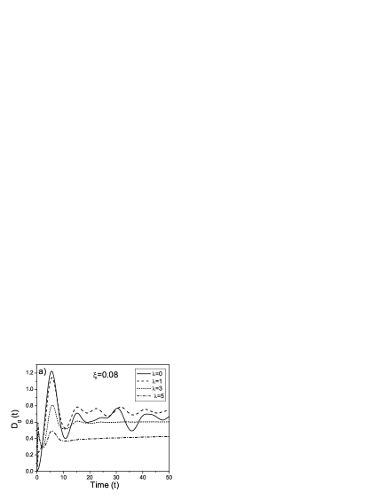
Figure 9: Time dependence of ${\cal D}_{g}$ for the nearest neighbor correlation (a) and global correlation (b). The period of oscillations scales as $1/\sqrt{\xi}$ and the amplitude is finite even without interaction $\lambda=0$. At large $\lambda$ ${\cal D}_{g}(t)$ saturates very fast similarly to the flat potential. At intermediate coupling $\lambda\sim 1$, however, the oscillations become more pronounced than in the noninteracting regime.

Interesting things happen if we turn on the interaction. In particular, if $\lambda$ is of the order of one, the oscillations become much more pronounced and smooth compared to noninteracting case (see Fig. 9). This is at first quite an unexpected result, since we know that the interaction leads to decoherence and saturation of ${\cal D}_{g}$. However this is not the whole story. In the previous analysis we saw that at least for the ${\cal D}_{g}(t)$, interaction “kills” high frequency contributions first. But that is precisely what we need for harmonic behavior. So crudely speaking, small or intermediate interaction removes harmonics causing dephasing of the noninteracting function ${\cal D}_{g}$. If interactions become strong $\lambda\gg 1$, then the noninteracting picture is irrelevant and we come back to the usual behavior with fast saturation of ${\cal D}_{g}$. Notice from Fig 9, that the noninteracting and interacting pictures are quite different at small time. This can be also understood naturally as a result of interplay of many harmonics at early stage of the evolution. Hence we expect that the typical time scale for the first maximum in the interacting problem will be of the order of the tunnelling time, which is much shorter than inverse level spacing. However at later times only slow harmonics survive leading to slight modifications of the noninteracting picture.

III.2 Modulated phase initial state

It is also straightforward to generalize the discussion of Section II.2 to the case of the periodic lattice. Namely, if the number of wells is even, then the state with a relative phase shift $\pi$, and equal numbers of bosons in the wells, is metastable for weak interaction. If $\lambda$ increases gradually, then when it reaches a critical value $\lambda_{c}$, this state becomes unstable Wu ; Smerzi . The critical value of $\lambda$ can be found from the linear analysis of (32) near the $\pi$ state Wu ; Smerzi :

$$\psi_{j}(t)\approx{\rm e}^{i\pi j-i(2+\lambda)t}\left(1+u{\rm e}^{iqj-i\omega t}+v^{\star}{\rm e}^{-iqj-i\omega t}\right),$$ (59)

where $u$ and $v$ are the small amplitudes and $q\neq 0$ is the wave vector of the perturbation. Substitution of this expansion into (32) gives the following secular equation for the eigenfrequencies $\omega$:

$$\left|\begin{array}[]{cc}\omega+2-2\cos q-\lambda&-\lambda\\ -\lambda&-\omega+2-2\cos q-\lambda\end{array}\right|=0,$$ (60)

which has two solutions

$$\omega=\pm 2\sqrt{(1-\cos{q})^{2}-\lambda(1-\cos q)}$$ (61)

Clearly $\omega$ is real if $\lambda<1-\cos q$. Otherwise, fluctuations with wavevector $q$ become unstable since the frequency becomes complex. The lowest nonzero $q$ for the periodic boundary conditions is $2\pi/M$, so the critical value of the interaction, where the $\pi$ state becomes the saddle point rather than local minimum is

$$\lambda_{c}=2\sin^{2}{\pi\over M}.$$ (62)

Similar to the two well case, the bosons undergo a spontaneous transition to the superposition of states, where all of them are in one of the wells. The time dependence of the variance of $N$ is analogous to that plotted on the top graph of Fig 4 (see Fig 10). We remark that a “slow” or adiabatic increase of interaction must be understood carefully. In the GP picture, an adiabatic increase of interaction means that the characteristic time scale is much smaller than the tunnelling time: $(d\ln\lambda/dt\ll 1)$. On the other hand, for the quantum problem adiabaticity would imply that $d\ln\lambda/dt$ is much smaller than the level spacing, which is proportional to inverse number of bosons. If the interaction is increased adiabatically in the quantum mechanical sense, then the system would follow the local minimum of the metastable state, and when $\lambda$ becomes larger than the critical value, it will undergo a spontaneous transition to the dipole state (or a superposition of the dipole states) with broken translational symmetry.

Figure 10: Sum of the squares of number of bosons in different lattice cites (with normalization $\sum_{j}n_{j}=1$). Clearly uniform distribution is stable until interaction is smaller than the critical value 62. At $t\to\infty$ we have $\sum_{j}~{}n_{j}^{2}~{}\to~{}1$ implying that all the bosons populate one of the wells.

IV Conclusions

We have studied the non-equilibrium temporal behavior of coupled bosons in a lattice. We predicted dynamical restoration of the phase coherence after a sudden increase of the tunnelling in a system initially in a Mott insulating state. In the strongly interacting case, $\lambda\gg 1$, the coherence reaches a steady state rapidly (within a Josephson time). On the other hand, time evolution in the weakly interacting regime $\lambda\lesssim 1$ depends strongly on the details of the confining potential. We predicted that in a parabolic potential $V_{j}=\xi j^{2}/2$ the coherence exerts decaying oscillations with period $T\propto 1/\sqrt{\xi}$ (see (58)). The period and the amplitude of oscillations only depend weakly on interaction in this case. On the other hand, if the confining potential is flat, then the oscillations are either periodic (for a particular number of wells in a lattice) or chaotic. Here the interaction leads to the decay of the oscillations with time. In both cases the system ultimately reaches steady state with nonzero coherence (dynamical Bose Einstein condensate).

For the two well case we explicitly tested the validity of GP approach. It was shown that the mapping of the deterministic quantum mechanical motion to the stochastic GP equations is essentially exact for time less than the characteristic inverse level spacing $t<N/\lambda$. Apart from the slight renormalization of the overall constant, the mapping is excellent in this time domain already for two bosons per well. For stronger interactions, the semiclassical and quantum mechanical trajectories start to depart faster, as expected.

We also considered the dynamical appearance of “Schrödinger cat” state under a slow increase of interaction from an initial phase modulated $\pi$ state. The $\pi$ state is stable while interaction is weak and becomes unstable when $\lambda>\lambda_{c}$. In the GP picture, this instability leads to the symmetry breaking, so that all the bosons spontaneously populate one of the wells. Quantum mechanically this means that the final configuration is the superposition of states in which bosons occupy different lattice sites. This approach can be used experimentally for the creation of strongly entangled states.

Appendix A Mean field ground state of the boson lattice system in a parabolic potential

The problem of the Mott insulator transitions for infinite arrays of bosons have been extensively studied during the last decade, see for example Fisher ; Sachdev ; Monien . It was shown Sachdev that the mean filed calculations qualitatively captures the two possible phases and gives a good estimate for the phase boundary. Recently, using quantum Monte-Carlo methods, an exact ground state for the system of bosons in a parabolic potential was found Troyer . It was shown that near the expected transition, the global compressibility does not vanish due to the spatial inhomogeneity. However, still the bosons form local insulating domains separated by narrow superfluid regions. The Monte Carlo approach, though very powerful, is incapable to solving the problem with many bosons per well. Therefore we think that for qualitative understanding of the ground state as a function of the interaction strength, it is worthwhile to do a mean field calculation.

The details of the derivation of the mean field equations can be found in Ref. Sachdev, . Here we will only outline the principal steps.

The mean field version of the free energy, corresponding to (1) is

$${\cal H}_{mf}= -\sum_{j}J(b_{j}a_{j}^{\dagger}+b_{j}^{\star}a_{j})+(V_{j}-\mu)a_{j}^{\dagger}a_{j}$$ (63)

$$+{U\over 2}a_{j}^{\dagger}a_{j}(a_{j}^{\dagger}a_{j}-1),$$

where $\mu$ is the chemical potential. The variational parameter $b_{j}$, corresponding to the ground state is:

$$b_{j}={\langle a_{j+1}+a_{j-1}\rangle\over 2},$$ (64)

where the average is taken in the ground state of (63). We can define the order parameter

$$\rho={\sum_{j}b_{j}^{\star}b_{j}}.$$ (65)

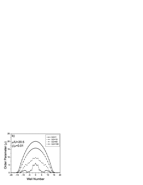
Figure 11: Mean field order parameter for different interactions in a parabolic potential ($V_{j}=\xi j^{2}/2$). Graph (a) corresponds to few bosons per site and the other two graphs do to many bosons.

The self consistent evaluation of the mean field $b_{j}$ is straightforward and the resulting order parameter is plotted in Fig 11. The graph (a) corresponds to few bosons per lattice site. If the interaction ($U$) is strong enough, then the order parameter forms a domain structure similar to that predicted in Troyer . For a large number of bosons per well, the quantum fluctuations start playing a role when $U$ becomes of the order of the number of bosons in the central well ($N\approx\mu/U$), and the smooth GP shape of boson density ($\rho$) breaks down. For very strong interaction, the actual profile of $\rho$ becomes sensitive to small variations of the mean density of bosons per central well.

Appendix B Amplitude fluctuations near the superfluid-insulator transition

This appendix reviews results on the damping of the amplitude oscillation mode near the superfluid-insulator transition, motivated by the recent paper of Altman and Auerbach aa . As we discussed in Section I.1, we have considered a system deep in the Mott insulating phase (with $\lambda\gg\lambda_{SI}$) taken suddenly to parameters for which the ground state was deep in the superfluid phase (with $\lambda\ll\lambda_{SI}$), while Altman and Auerbach consider the case when both the initial and final values of $\lambda$ were not too far from $\lambda_{SI}$, but remained on opposite sides of it.

A key ingredient in the dynamics of the amplitude mode for $\lambda<\lambda_{SI}$ is the damping induced by emission of the Goldstone “spin wave” or “phonon” modes. This problem was considered in Refs. ssrelax, ; sscrit, , and it was found that the amplitude oscillations were overdamped in the $\lambda<\lambda_{SI}$ scaling limit associated with the second-order superfluid-insulator transition. We will review these results below, and display expressions which also allow us to move beyond the scaling limit to values of $\lambda$ much smaller than $\lambda_{SI}$ (see 73); the amplitude mode can become oscillatory in the latter regime ssrelax ; aa . This also consistent with the considerations of the present paper, where we have found that the oscillations of the superfluid coherence were present in the parabolic multiwell case for $\lambda=5$ in Fig 9, but were fully overdamped for $\lambda=10$ (not shown). We found similar behavior in the complete quantum solution for the two-well problem—however in the latter case, the oscillations reappeared at very large $\lambda\sim N^{2}$: these are the “number” oscillations of the Mott insulator, and were also found in Ref. ssrelax, . The fate of these very small and very large $\lambda$ oscillations in the multiwell case near $\lambda_{SI}$ requires a treatment of the interacting quantum dynamics: this was done in Refs. ssrelax, ; sscrit, , and the results are reviewed here.

As is well known, we can describe the superfluid-insulator transition by the $N=2$ case of the $N$-component $\varphi^{4}$ field theory, where the superfluid order parameter $\psi$ in Section I

$$\psi\sim\varphi_{1}+i\varphi_{2}$$ (66)

. The action for $\lambda$ close to $\lambda_{SI}$ is

$$\mathcal{S} = \int d^{d}xd\tau\Biggl{[}\frac{1}{2}\left(\nabla_{x}\varphi_{\alpha}\right)^{2}+\frac{1}{2c^{2}}\left(\partial_{\tau}\varphi_{\alpha}\right)^{2}-\frac{(r_{c}+s)}{2}\varphi_{\alpha}^{2}$$ (67)

$$~{}~{}~{}~{}~{}~{}~{}~{}~{}~{}~{}~{}+\frac{u}{2N}\left(\varphi_{\alpha}^{2}\right)^{2}\Biggr{]},$$

where $\alpha=1\ldots N$, $c$ is a velocity, $d$ is the spatial dimensionality and $u$ is a quartic non-linearity. The coefficient of $\varphi_{\alpha}^{2}$ is used to tune the system across the transition, and the value of $r_{c}$ is chosen to that the transition occurs at $s=0$ i.e. $s\sim\lambda-\lambda_{SI}$. We assume that in the superfluid phase $\langle\varphi_{\alpha}\rangle=N_{0}\delta_{\alpha,1}$. The oscillations of the spin-wave modes are given by the transverse susceptibility $\chi_{\perp}(k,\omega)$, while those of the amplitude mode are given by the longitudinal susceptibility $\chi_{\parallel}(k,\omega)$; here $k$ is a wavevector, $\omega$ is a frequency, and the susceptibilities are defined by

$$\chi_{\perp}(k,\omega) = \left\langle\left|\varphi_{2}(k,\omega)\right|^{2}\right\rangle$$

$$\chi_{\parallel}(k,\omega) = \left\langle\left|\varphi_{1}(k,\omega)\right|^{2}\right\rangle-N_{0}^{2}(2\pi)^{d+1}\delta(k)\delta(\omega)~{}~{}$$ (68)

Expressions for $\chi_{\perp,\parallel}$ were given in Refs. ssrelax, ; sscrit, using both perturbation theory in $u$ and the large $N$ expansion. Here, we collect them with a common notation, and interpret them in the present context. To first order in $u$, the position of the critical point is determined by

$$r_{c}=\frac{2u(N+2)c}{N}\int\frac{d^{d+1}p}{(2\pi)^{d+1}}\frac{1}{p^{2}}$$ (69)

where $p=(k,-i\omega/c)$ is the $(d+1)$-dimensional Euclidean momentum. In the limit of large $N$, but $u$ arbitrary, the value of $r_{c}$ is given simply by the $N\rightarrow\infty$ limit of (69). To first order in $u$, we obtain for $\chi_{\perp}$

$$\chi_{\perp}^{-1}(p)=p^{2}-\frac{8csu}{N}\int\frac{d^{d+1}q}{(2\pi)^{d+1}}\frac{1}{q^{2}+2s}\left(\frac{1}{(p+q)^{2}}-\frac{1}{q^{2}}\right),$$ (70)

where $q$ is also a $(d+1)$-dimensional Euclidean momentum; at $N=\infty$ we have simply $\chi_{\perp}^{-1}(p)=p^{2}$. The expression (70) describes the spin-wave oscillations, along with their essentially negligible damping from their coupling to the amplitude mode (as can be verified by taking the imaginary part of the loop integral in (70) after analytic continuation to real frequencies).

The damping in the longitudinal modes is much more severe, and we will consider it explicitly. To first, order in $u$, we obtain the expression

$$\chi_{\parallel}^{-1}(p)=p^{2}+2s-\frac{4csu(N-1)}{N}\Pi(p)+\delta\chi_{\parallel}^{-1}(p).$$ (71)

Here the strong damping term has been included in $\Pi(p)$ whose explicit form is discussed below in (74), while $\delta\chi_{\parallel}$ contains additional non-singular terms we can safely neglect. For completeness, we give the expression for the latter

$$\delta\chi_{\parallel}^{-1}(p) = \frac{12uc}{N}\int\frac{d^{d+1}q}{(2\pi)^{d+1}}\left(\frac{1}{q^{2}}-\frac{1}{q^{2}+2s}\right)$$

$$- \frac{36csu}{N}\int\frac{d^{d+1}q}{(2\pi)^{d+1}}\frac{1}{(q^{2}+2s)((p+q)^{2}+2s)};$$

note that these terms always involve coupling to an amplitude mode fluctuation (with “mass” $2s$) and this is the reason their contribution is non-singular. We find below in (74) that the $\Pi(p)$ contribution in (71) involves only spin-wave fluctuations and hence it becomes very large at low frequencies, where the perturbative expansion in (71) can no longer be trusted. Fortunately, a resummation of these singular corrections is provided by the large $N$ expansion, which yields

$$\chi_{\parallel}^{-1}(p)=p^{2}+\frac{2s}{1+2cu\Pi(p)};$$ (73)

it is satisfying to check that (73) and (71) are entirely consistent with each other in their overlapping limits of validity of small $u$ and large $N$. The expression (73) was given earlier ssrelax in the scaling limit, which corresponds to ignoring the 1 in the denominator because $\Pi(p)$ becomes large. The utility of (73) is that it does not have divergent behavior at small $p$.

We turn, finally, to the expression for $\Pi(p)$, which is

$$\Pi(p) = \int\frac{d^{d+1}q}{(2\pi)^{d+1}}\frac{1}{q^{2}(p+q)^{2}}$$ (74)

$$= F_{d}|p|^{d-3},$$

where $F_{d}$ is a numerical prefactor which is not difficult to obtain explicitly. Notice that $\Pi(p)$ is singular as $p\rightarrow 0$ in $d<3$, and this is the reason for the strong damping of the amplitude mode. After analytic continuation to real frequences, we have in $d=2$

$$\Pi(k,\omega)=\frac{1}{8\sqrt{k^{2}-(\omega/c)^{2}}}~{}~{}~{};~{}~{}~{}d=2;$$ (75)

this has a non-zero imaginary part for $\omega>ck$ which leads to the damping of the amplitude mode. The expression for $\Pi(p)$ is infrared divergent in $d=1$, and this is the signal that there is no true long-range order; nevertheless, its imaginary part remains well defined as $d\searrow 1$, and we find

$$\mbox{Im}\Pi(k,\omega)=\frac{1}{4((\omega/c)^{2}-k^{2})}\theta(\omega-ck)~{}~{}~{};~{}~{}~{}d=1$$ (76)

which again predicts strong damping at low frequencies. The expressions (73-76) can be used to describe the evolution of the weakly damped amplitude mode at $\omega=\sqrt{c^{2}k^{2}+2s}$ at large $s$ deep in the superfluid, to the overdamped mode with no sharp resonance at this frequency for small $s$.

References

- (1) C. Orzel, A. K. Tuchman, M. L. Fenselau, M. Yasuda, and M. A. Kasevich, Science 291, 2386 (2001).
- (2) M. Greiner, O. Mandel, T. Esslinger, T. W. Hänsch, and I. Bloch, Nature, 415, 39 (2002).
- (3) M. P. A. Fisher, P. B. Weichman, G. Grinstein, D. S. Fisher, Phys. Rev. B 40, 546 (1989).
- (4) S. Sachdev, Quantum Phase Transitions, Cambridge University Press, Cambridge (1999).
- (5) J. K. Fredericks, H. Monien, Europhys. Lett. 26, 545 (1994).
- (6) N. Elstner and H. Monien, Phys. Rev. B 59, 12184 (1999).
- (7) L. Amico and V. Penna, Phys. Rev. B 62, 1224 (2000).
- (8) D. Jaksch, C. Bruder, J. I. Cirac, C. W. Gardiner, and P. Zoller, Phys. Rev. Lett. 81, 3108 (1998).
- (9) M. Kramer, L. Pitaevkii, and S. Stringari, Phys. Rev. Lett. 88, 180404 (2002).
- (10) R. Franzosi and V. Penna, cond-mat/0205209.
- (11) J. Dziarmaga, A. Smerzi, W. H. Zurek, and A. R. Bishop, Phys. Rev. Lett. 88, 167001 (2002).
- (12) A. Trombettoni, A. Smerzi, and A. R. Bishop, Phys. Rev. Lett. 88, 173902 (2002).
- (13) G. G. Batrouni, V. Rousseau, R. T. Scalettar, M. Rigol, A. Muramatsu, P. J. H. Denteneer, and M. Troyer, cond-mat/0203082 (2002).
- (14) V. A. Kashurnikov, N. V. Prokof’ev, and B. V. Svistunov, condmat/0202510.
- (15) A. Tuchman, S. Dettmer, M. Fenselau and M. Kasevich, to appear.
- (16) K. Damle, S. Majumdar, and S. Sachdev, Phys. Rev. A 54, 5037 (1996); K. Damle, T. Senthil. S. Majumdar, and S. Sachdev, Europhys. Lett. 36, 7 (1996).
- (17) E. Altman and A. Auerbach, cond-mat/0206157.
- (18) S. Sachdev, Phys. Rev. B 59, 14054 (1999).
- (19) J. R. Anglin and A. Vardi, Phys. Rev. A 64, 013605 (2001).
- (20) S. Raghavan, A. Smerzi, S. Fantoni, and S. R. Shenoy, Phys. Rev. A59, 620 (1999).
- (21) S. Sachdev, K. Sengupta and S. M. Girvin, Phys. Rev. B to appear, cond-mat/0205169.
- (22) M. Kasevich, private communication.
- (23) G. J. Milburn, J. Corney, E. M. Wright, and D. F. Walls, Phys. Rev. A 55, 4318 (1997).
- (24) B. Wu and Q. Niu, Phys. Rev. A 64, 061603, (2001).
- (25) A. Smerzi, A. Trombettoni, P. G. Kevrekidis and A. R. Bishop, Phys. Rev. Lett. in press.
- (26) S. Sachdev, Phys. Rev. B 55, 142 (1997).