Infinite chain of $N$ different deltas: A simple model for a quantum wire

Abstract

We present the exact diagonalization of the Schrödinger operator corresponding to a periodic potential with $N$ deltas of different couplings, for arbitrary $N$. This basic structure can repeat itself an infinite number of times. Calculations of band structure can be performed with a high degree of accuracy for an infinite chain and of the correspondent eigenlevels in the case of a random chain. The main physical motivation is to modelate quantum wire band structure and the calculation of the associated density of states. These quantities show the fundamental properties we expect for periodic structures although for low energy the band gaps follow unpredictable patterns. In the case of random chains we find Anderson localization; we analize also the role of the eigenstates in the localization patterns and find clear signals of fractality in the conductance. In spite of the simplicity of the model many of the salient features expected in a quantum wire are well reproduced.

         PACS Numbers: 03.65.-w: Quantum Mechanics

                              71.23.An: Theories and Models; Localized States

                              73.21.Hb: Quantum Wires

Quantum wires represent the dreamed idea of make a conductor wire as small as a molecule. The idea that macroscopic devices we have been using for years can actually be built in nature at the nanoscale size goes back to Feynman and is the basis of all work currently carried out in the field of Quantum Electronics. This area of research is not only interesting in itself from the fundamental point of view but has also profound implications in applied physics and material sciences as hundreds of experiments are being carried out nowdays with a high degree of success. The purpose of this paper is to show that some of the ideas underlying the actual development of different types of quantum wires can actually be modelled in quite a simple manner using elementary quantum mechanics. This is specially important from our point of view as it provides a bridge between current fundamental research and basic concepts of quantum mechanics which are usually the subject of graduate standard programs.

The aim to modelate a simple one-dimensional solid in order to study its band structure goes back to Kronig and Penney in the thirties [KP] but since then much work has been done along the lines of this first seminal reference. A sample of the variety of models that can be constructed with the same ideas can be found in [LM]. As the main interest of almost all of these authors was band theory, the techniques used in all these papers were mainly addressed to semiconductor physics [altman]. Much more recently a revival of the same models and techniques [SZML] has arisen as a consequence of the interest in truly theoretical and experimental one-dimensional physical systems from which quantum wires are just only one example [CDEK]. Right now the research in molecular conductances, one-dimensional metallic rings and other devices of the same sort lends support to the idea of generalizing old methods yielding exact analitic solutions coupled to the use of desk-top computer algebra.

Here firstly we shall solve analitically the band structure of an infinite periodic chain of delta potentials each one with a different coupling inside the primitive cell paying mostly attention to the mathematical aspects. After studing the band structure of the chain one can introduce randomness boosted by quantum fluctuations in order to account for localization. Fortunately the model seems rich enough to yield more information such as the generalization of the Saxon-Hutner conjecture [SH] and even scaling exhibited as fractal behaviour of the conductance [Hegger]. The Paper will be organized as follows. In Section I we shall present the analytic solution of the periodic case of infinite different delta potentials. The band structure of this one dimensional Periodic Potential will also be briefly discussed. In Section II we turn our attention to the case of random arrays of one dimensional delta potentials with different couplings. Here we discuss the density of states using the functional equation method and classify the different types of localization appearing when disorder is present. As we have been able to increase our understanding of localization to the extent of detecting universality effects, we shall entirely devote the Section III to the discussion of fractality in the conductance and the different checkings we have managed to perform in order to ascertain ourselves and try to convince the reader that the effect is present even in this extremely simple model. We close with a Section of Conclusions.

1 Periodic Array

Let us consider an electron in a periodic one dimensional chain of atoms modelled by the potential constituted by an array of $N$ delta functions each one with its own coupling $e_{i}^{2}$, ($i=1,2,...N$). After finishing the $N$-array, the structure repeats itself an infinite number of times. The number of species $N$, can be arbitrarily large but finite. The case $N$=1 is an old textbook exercise but may be convenient to be revisited [FLUG] for taking a full profit of our general results. The generalization can thus be followed in a more straightforward manner. The relevant primitive cell for $N=2$ can be represented for the following set of wavefunctions:

primitive cell $$\begin{cases}\Psi_{1}(x)\,=\,A_{1}e^{ikx}+B_{1}e^{-ikx}\qquad&0\leq x<a\\ \Psi_{2}(x)\,=\,A_{2}e^{ik(x-a)}+B_{2}e^{-ik(x-a)}\qquad&a\leq x<2a\end{cases}$$

$$\quad\Psi_{3}(x)\,=\,e^{2iQa}\left[A_{1}e^{ik(x-2a)}+B_{1}e^{-ik(x-2a)}\right]$$

The matrix relating the amplitudes of the above wave functions for this $N=2$ case can be written as:

$$\begin{pmatrix}e^{ika}&e^{-ika}&\begin{picture}(0.0,0.0)(0.0,70.0)\dottedline{4}(0,15)(0,75)\end{picture}&-1&-1\\ -ike^{ika}&ike^{-ika}&&\big{(}ik-{2\over a_{1}}\big{)}&-\big{(}ik+{2\over a_{1}}\big{)}\vspace{-2mm}\\ \begin{picture}(0.0,0.0)(100.0,0.0)\dottedline{4}(80,0)(335,0)\end{picture}\\ -\mathcal{F}_{2}&-\mathcal{F}_{2}&&e^{ika}&e^{-ika}\\ \big{(}ik-{2\over a_{2}}\big{)}\mathcal{F}_{2}&-\big{(}ik+{2\over a_{2}}\big{)}\mathcal{F}_{2}&&-ike^{ika}&ike^{-ika}\end{pmatrix}$$ (1)

It is trivial to generalize these two steps to the case of three species (i.e. $N=3$). One can equally write the correspondent matrix in the form:

$$\begin{pmatrix}e^{ika}&e^{-ika}&\begin{picture}(0.0,0.0)(0.0,90.0)\dottedline{4}(0,0)(0,95)\end{picture}&-1&-1&\begin{picture}(0.0,0.0)(0.0,90.0)\dottedline{4}(0,0)(0,95)\end{picture}&0&0\\ -ike^{ika}&ike^{-ika}&&\big{(}ik-\frac{2}{a_{1}}\big{)}&-\big{(}ik+\frac{2}{a_{1}}\big{)}&&0&0\vspace{-2mm}\\ \begin{picture}(0.0,0.0)(20.0,0.0)\dottedline{4}(0,0)(380,0)\end{picture}\\ 0&0&&e^{ika}&e^{-ika}&&-1&-1\\ 0&0&&-ike^{ika}&ike^{-ika}&&\big{(}ik-\frac{2}{a_{2}}\big{)}&-\big{(}ik+\frac{2}{a_{2}}\big{)}\vspace{-2mm}\\ \begin{picture}(0.0,0.0)(20.0,0.0)\dottedline{4}(0,0)(380,0)\end{picture}\\ -\mathcal{F}_{3}&-\mathcal{F}_{3}&&0&0&&e^{ika}&e^{-ika}\\ \big{(}ik-\frac{2}{a_{3}}\big{)}\mathcal{F}_{3}&-\big{(}ik+\frac{2}{a_{3}}\big{)}\mathcal{F}_{3}&&0&0&&-ike^{ika}&ike^{-ika}\end{pmatrix}$$ (2)

where in all of the above cases, we have used the notation:

$$\mathcal{F}_{N}=\exp\{iNQa\}\quad\text{and}\quad Q\in\left[-\frac{\pi}{Na},\frac{\pi}{Na}\right)$$ (3)

and we shall also be using the length of each species, defined as:

$$a_{i}=\frac{\hslash^{2}}{me_{i}^{2}}$$ (4)

One can now proceed to the generalization of the matrix form for general number $N$ of species just by defining the following $2\negmedspace\times\negmedspace 2$ matrices:

$$\mathbf{E}\,=\,\begin{pmatrix}e^{ika}&e^{-ika}\\ -ike^{ika}&ike^{-ika}\end{pmatrix}\quad;\quad\mathbf{A_{j}}\,=\,\begin{pmatrix}-1&-1\\ \big{(}ik-\frac{2}{a_{j}}\big{)}&-\big{(}ik+\frac{2}{a_{j}}\big{)}\end{pmatrix}.$$ (5)

The matrices for $N=2$ and $N=3$ species given by (1) and (2) can now be put in a more compact form with the help of the $\mathbf{E}$ and $\mathbf{A_{j}}$ as:

$$\begin{pmatrix}\mathbf{E}&\mathbf{A_{1}}\\ \mathbf{A_{2}}\mathcal{F}_{2}&\mathbf{E}\end{pmatrix}_{4\times 4}\quad;\quad\begin{pmatrix}\mathbf{E}&\mathbf{A_{1}}&0_{2\times 2}\\ 0_{2\times 2}&\mathbf{E}&\mathbf{A_{2}}\\ \mathbf{A_{3}}\mathcal{F}_{3}&0_{2\times 2}&\mathbf{E}\end{pmatrix}_{6\times 6}$$ (6)

It is now relatively simple to guess that the general form of a matrix for $N$ species must be written as:

$$\begin{pmatrix}\mathbf{E}&\mathbf{A_{1}}&0_{2\times 2}&{3}&0_{2\times 2}\\ 0_{2\times 2}&\mathbf{E}&\mathbf{A_{2}}&0_{2\times 2}&{2}&0_{2\times 2}\\ \vdots&0_{2\times 2}&\mathbf{E}&\mathbf{A_{3}}&0_{2\times 2}&{1}&0_{2\times 2}\\ \vdots&\vdots&0_{2\times 2}&\ddots&\ddots&\ddots&\vdots\\ \vdots&\vdots&\vdots&\ddots&\ddots&\ddots&0_{2\times 2}\\ 0_{2\times 2}&\vdots&\vdots&&\ddots&\mathbf{E}&\mathbf{A_{N-1}}\\ \mathcal{F}\mathbf{A_{N}}&0_{2\times 2}&0_{2\times 2}&{2}&0_{2\times 2}&\mathbf{E}\end{pmatrix}_{2N\times 2N}$$ (7)

So far nothing very exciting has happened except that one can write the matrices in a compact, logic and generalizable way. And in fact without further steps the progress would have not been certainly remarkable. The real breakthrough arises when one realizes that one has to deal with the determinants equated to zero of these matrices in order to learn something about the band condition of this one dimensional N-species quantum periodic structure. Let us define the following function $(\epsilon=ka)$ :

$$h_{i}(\epsilon)=\cos(\epsilon)+\left(\frac{a}{a_{i}}\right)\frac{\sin(\epsilon)}{\epsilon}$$ (8)

A quite simple computer algebra calculation shows that the determinant equated to zero of (1), which belongs to the $N=2$ case, can be written in terms of these functions as

$$\cos(2Qa)=2h_{1}h_{2}-1$$ (9)

And the determinant of the $N=3$ matrix given by (2) can also be calculated to yield:

$$\cos(3Qa)=4h_{1}h_{2}h_{3}-(h_{1}+h_{2}+h_{3})$$ (10)

Below, the cases $N=4,5,6$ and 7 are explicitely listed, using the generalized matrix (7) for each case and calculating the determinant equated to zero with the help of the $h(\epsilon)$ functions (8). The result is:

$$\cos(4Qa)\,=\,8\;h_{1}h_{2}h_{3}h_{4}-2\;\big{(}h_{1}h_{2}+h_{1}h_{4}+h_{2}h_{3}+h_{3}h_{4}\big{)}+1$$ (11)

$$\cos(5Qa)\,=\,16\;h_{1}h_{2}h_{3}h_{4}h_{5}-4\;\big{(}h_{1}h_{2}h_{3}+h_{1}h_{2}h_{5}+h_{1}h_{4}h_{5}+\\ h_{2}h_{3}h_{4}+h_{3}h_{4}h_{5}\big{)}+\big{(}h_{1}+h_{2}+h_{3}+h_{4}+h_{5}\big{)}$$ (12)

$$\cos(6Qa)\,=\,32\;h_{1}h_{2}h_{3}h_{4}h_{5}h_{6}-8\,\big{(}h_{1}h_{2}h_{3}h_{4}+h_{1}h_{2}h_{3}h_{6}+h_{1}h_{2}h_{5}h_{6}\,+\\ +h_{1}h_{4}h_{5}h_{6}+h_{2}h_{3}h_{4}h_{5}+h_{3}h_{4}h_{5}h_{6}\big{)}+2\;\big{(}h_{1}h_{2}+h_{1}h_{4}+h_{1}h_{6}\,+\\ +h_{2}h_{3}+h_{2}h_{5}+h_{3}h_{4}+h_{3}h_{6}+h_{4}h_{5}+h_{5}h_{6}\big{)}-1$$ (13)

$$\cos(7Qa)\,=\,64\;h_{1}h_{2}h_{3}h_{4}h_{5}h_{6}h_{7}-16\;\big{(}h_{1}h_{2}h_{3}h_{4}h_{5}+h_{1}h_{2}h_{3}h_{4}h_{7}\,+\\ +h_{1}h_{2}h_{3}h_{6}h_{7}+h_{1}h_{2}h_{5}h_{6}h_{7}+h_{1}h_{4}h_{5}h_{6}h_{7}+h_{2}h_{3}h_{4}h_{5}h_{6}+h_{3}h_{4}h_{5}h_{6}h_{7}\big{)}\,+\\ +4\;\big{(}h_{1}h_{2}h_{3}+h_{1}h_{2}h_{5}+h_{1}h_{2}h_{7}+h_{1}h_{4}h_{5}+h_{1}h_{4}h_{7}+h_{1}h_{6}h_{7}+h_{2}h_{3}h_{4}\,+\\ +h_{2}h_{3}h_{6}+h_{2}h_{5}h_{6}+h_{3}h_{4}h_{5}+h_{3}h_{4}h_{7}+h_{3}h_{6}h_{7}+h_{4}h_{5}h_{6}+h_{5}h_{6}h_{7}\big{)}\,-\\ -\big{(}h_{1}+h_{2}+h_{3}+h_{4}+h_{5}+h_{6}+h_{7}\big{)}.$$ (14)

We have been able to proof by induction that the general form of the $N$ species case can be given as:

$$\cos(NQa)\,=\,\mathcal{B}(\epsilon;a_{1},\ldots,a_{N})$$ (15)

• $N$ even
  B(ϵ;a_1,…,a_N) = 2^N-1∑_Ph_i…(N)…h_k  -  2^N-3∑_P h_i…(N-2)…h_k  + 
  +  2^N-5∑_P h_i…(N-4)…h_k  - …(-1)^N2-1  2 ∑_P h_i…(2)…h_k  +  (-1)^N2

• $N$ odd
  B(ϵ;a_1,…,a_N) = 2^N-1∑_Ph_i…(N)…h_k  -  2^N-3∑_P h_i…(N-2)…h_k  +
  +  2^N-5∑_P h_i…(N-4)…h_k  - …(-1)^N-32  2^2 ∑_P h_i…(3)…h_k  +
  (-1)^N-12(h_1+h_2+h_3+…+h_N)

All what remains is to define the symbol $\sum_{P}h_{i}...(M)...h_{k}$ which means the sum of all possible products of M different $h_{i}$’s with the following rule for each product: the indices must follow an increasing order and to an odd index must always follow an even index and reciprocally.

The band structure provided by (• ‣ 1) and (• ‣ 1) is not just exact but also extremely useful from the point of view of computer algebra calculations. In fact we have carried out various profiles for the curves provided for these conditions until $N$=30 or more using just few seconds of a lap-top regular computer. The reason for that lies mainly in the systematic use of the form, products and combinations of the $h(\epsilon)$-function defined by (8). As examples of what has just been said we list in Fig. 1 and 2 a series of band curves for large number of species and various values of the parameter $\left(\frac{a}{a_{i}}\right)$, defining the characteristic value of the $h(\epsilon)$-function.

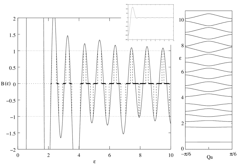
Figure 1: Band condition (detail in inset) and band structure (1BZ) for a periodic chain with six species in the primitive cell $\big{(}\frac{a}{a_{i}}\big{)}$: 2, 2.5, 1, 1.5, -1, -2.

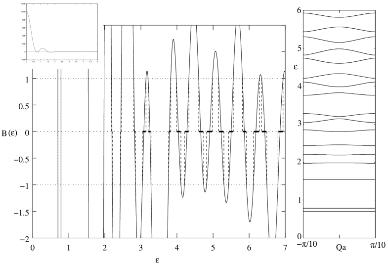
Figure 2: Band condition (detail in inset) and band structure (1BZ) for a periodic chain with ten species in the primitive cell $\big{(}\frac{a}{a_{i}}\big{)}$: 1, 2, 3, -1, -2, -3, 0.5, -0.5, 2, 1.

(a) Two species $\big{(}\frac{a}{a_{i}}\big{)}$: -0.3,-0.9

(b) Four species $\big{(}\frac{a}{a_{i}}\big{)}$: -3, -5, -6, -4

Figure 3: Density of electronic states for different configurations of the primitive cell.

One can observe also the unpredictable set of allowed bands which appear at low energies. This pattern increases its unpredictibility with the number of species.

Once the band condition is known, one can write the distribution of electronic states in a very simple form. In one dimension the density of states per unit length of the chain for the n$th$ band comes from,

$$g_{n}(\epsilon)\,=\,\frac{1}{2\pi}\sum_{Q}\bigg{|}\frac{d\epsilon(Q)}{dQ}\bigg{|}^{-1}$$ (16)

where the sum is over all the first Brillouin zone (1BZ) points $Q$ with the same energy $\epsilon$. Due to the parity of $\cos(NQa)$ the number of points with the same value of $\epsilon$ in the 1BZ is always 2, and provided that overlapping of neighbouring bands is not possible in this system, we can write the density of states as

$$g(\epsilon)\,=\,\frac{1}{\pi}\bigg{|}\frac{dQ(\epsilon)}{d\epsilon}\bigg{|}$$ (17)

inside the permitted bands. From (15) a trivial calculation leads to,

$$G(\epsilon)\equiv g(\epsilon)\cdot a\,=\,\frac{\left[1-\mathcal{B}^{2}\right]^{-\frac{1}{2}}}{N\pi}\bigg{|}\frac{d\mathcal{B}(\epsilon)}{d\epsilon}\bigg{|}$$ (18)

where $G(\epsilon)$ is the density of electronic states per atom. Fig. 3 shows some examples of the characteristic form of the distribution of states for different configurations of the primitive cell.

2 Random Chains

The structures one can observe in Nature hardly show a perfect periodicity. Even in the laboratory it is a difficult task to grow a crystal free of impurities, vacancies or dislocations. We shall now treat the presence of substitutional disorder in one dimensional delta-potential chains, that is we consider a chain of equally spaced deltas in which the sequence of different species does not obey a periodic pattern. This model has been mainly studied regarding the vibrational spectrum [LM], paying less attention to its electronic density of states [AgaBor]. For the purpose of studying quantum wires the relevant behaviour we want to analyze lies more in the latter than in the former physical property.

2.1 Energy gaps

The Saxon and Hutner conjecture [SH] was proved by Luttinger for the case of binary chains [lutt]. We have been able to extend it to the general case. A detailed calculation following the line of Schmidt [Schmidt] can be found in Appendix LABEL:ap:gaps. The result can be easily summarized as follows: the forbidden bands that coincide in different one species delta chains with couplings $e_{1}^{2},\ldots,e_{N}^{2}$ are also forbidden levels in any infinite chain made up of deltas of the $N$ types. This conclusion can be applied to both disordered and periodic chains. As can be seen in the calculations the result requires the interatomic distances of the chains involved to be constant and the same for all of them.

2.2 Eigenenergies for finite disorder chains

Let us calculate the allowed energy levels of a finite non-periodic chain of deltas with fixed end-points boundary conditions. The procedure to follow is the same as for the periodic case but imposing the vanishing of the wave function at the end-points of the chain which we locate at one atomic distance to the left of the first delta and to the right of the last one. The connection of the wave function throughout the different sectors leads us to a condition for the permitted energy levels in the form of the determinant of a matrix equated to zero. Again these matrices can be written in a generalizable way. Thus for $N$ deltas we have

$$\begin{vmatrix}\mathbf{E}&\mathbf{A_{1}}&0_{2\times 2}&{3}&0_{2\times 2}\\ 0_{2\times 2}&\mathbf{E}&\mathbf{A_{2}}&0_{2\times 2}&{2}&0_{2\times 2}\\ \vdots&0_{2\times 2}&\mathbf{E}&\mathbf{A_{3}}&0_{2\times 2}&{1}&0_{2\times 2}\\ \vdots&\vdots&0_{2\times 2}&\ddots&\ddots&\ddots&\vdots\\ \vdots&\vdots&\vdots&\ddots&\ddots&\ddots&0_{2\times 2}\\ 0_{2\times 2}&\vdots&\vdots&&\ddots&\mathbf{E}&\mathbf{A_{N}}\\ \mathbf{U}&0_{2\times 2}&0_{2\times 2}&{2}&0_{2\times 2}&\mathbf{V}\end{vmatrix}_{2(N+1)\times 2(N+1)}\!=\,0.$$ (19)

whith $\mathbf{E}$ and $\mathbf{A_{j}}$ defined in (5) and

$$\mathbf{U}\,=\,\begin{pmatrix}1&1\\ 0&0\end{pmatrix}\qquad\mathbf{V}\,=\,\begin{pmatrix}0&0\\ e^{ika}&e^{-ika}\end{pmatrix}.$$ (20)

We found the condition to be factorizable in terms of the functions $h_{j}(\epsilon)$ in a similar manner to that of the periodic chain. The eigenenergies of the system are the roots of:

$$\sin(\epsilon)\cdot\mathcal{A}(\epsilon;a_{1},\ldots,a_{N})\,=\,0$$ (21)

where

• $N$ even
  A(ϵ;a_1,…,a_N) = 2^N (h_1⋅…⋅h_N)  -  2^N-2∑’_P h_i…(N-2)…h_k  + 
  &+ 2N-4∑’P hi…(N-4)…hk  - …(-1)N2-1  22 ∑’P hi…(2)…h