Signatures of a Concentration Dependent Flory $\chi$ Parameter: Swelling and Collapse of Coils and Brushes

Abstract

The quality of solvents of polymers is often described in terms of the Flory $\chi$ parameter typically assumed to depend only on the temperature, $T$. In certain polymer-solvent systems fitting the experimental data enforces the replacement of $\chi(T)$ by a concentration dependent $\chi_{eff}$. In turn, this modifies the swelling and collapse behavior. These effects are studied, in the framework of a mean-field theory, for isolated coils and for planar brushes. The $\phi$ dependence of $\chi_{eff}$ gives rise to three main consequences: (i) Shift in the cross-over between Gaussian and self-avoidance regimes; (ii) A possibility of first-order collapse transition for isolated flexible coils; (iii) The possibility of a first-order phase transition leading to a vertical phase separation within the brush. The discussion relates these effects directly to thermodynamic measurements and does not involve a specific microscopic model. The implementation for the case of Poly(N-isopropylacrylamide) (PNIPAM) is discussed.

I Introduction

The quality of solvents of polymers is often quantified in terms of the Flory free energy. In this free energy, the mixing energy term has the form $\chi\phi(1-\phi)$ where $\chi$ is the Flory interaction parameter and $\phi$ is the monomer volume fraction. $\chi$ and the related second virial coefficient, $v=1-2\chi$, measure the solvent quality. Thus $v>0$ corresponds to a good solvent, $v=0$ to a $\theta$ solvent while $v<0$ indicates a poor one. An important characteristic of these three regimes is the associated swelling behavior. Thus, the span of an isolated chain in the three regimes scales respectively as $N^{3/5}$, $N^{1/2}$ and $N^{1/3}$. Typically, it is assumed that $\chi$ depends only on the temperature, $\chi=\chi(T)$.[1, 2, 3, 4] However when thermodynamic data are analyzed in terms of the Flory free energy, it is often necessary to replace $\chi\phi(1-\phi)$ by $\chi_{eff}\phi(1-\phi)$ where $\chi_{eff}$ is a function of both $T$ and $\phi$ i.e., $\chi_{eff}=\chi_{eff}(T,\phi)$.[1, 5, 6, 7, 8] The introduction of $\chi_{eff}(T,\phi)$ requires, in turn, modification of the discussion of solvent quality. In the following we aim to clarify this issue by exploring some of the microscopic consequences of $\chi_{eff}(T,\phi)$.

The solvent quality of polymer solutions as characterized by $\chi_{eff}(T,\phi)$ concerns two issues: First, is the stability of the solution with respect to phase separation due to diffusion of chains. The second is the degree of swelling of polymer coils. While the first issue was analyzed in considerable detail,[9, 10, 11, 12] less attention was given to the second topic.[13, 14] The purpose of this article is to explore the signatures of $\chi_{eff}=\chi_{eff}(T,\phi)$ on the swelling behavior of isolated coils and of brushes of terminally anchored chains. In turn, these signatures of the solvent quality involve two aspects. One is a “global” solvent quality as revealed in systems of uniform density. To study this facet we consider the effect of $\chi_{eff}(\phi)$ on the swelling behavior in two cases: (i) an isolated coil within the Flory approximation[1, 2] and (ii) a brush as described by the Alexander model.[15, 16] As we shall discuss, the global solvent quality is characterized by $\overline{\chi}(\phi)=\chi_{eff}-(1-\phi)\partial\chi_{eff}/\partial\phi$ rather than by $\chi_{eff}(\phi)$. The $\phi$ dependence of $\overline{\chi}$ gives rise to two effects. First is a qualitative modification of the collapse transition that can assume, within these models, the character of a first-order phase transition. Second is a significant shift in the cross-over between the behavior of an ideal chain to that of a self-avoiding one. For systems involving gradients in $\phi$, it is necessary to consider a “local” solvent quality. In such systems $\overline{\chi}(\phi)$ is no longer the sole measure of the solvent quality. The local solvent quality is explored by using the Pincus approximation for brushes[17, 18] thus allowing for the concentration profile and its coupling with $\chi_{eff}(\phi)$.[19] The $\phi$ dependence of $\chi_{eff}$ gives rise to deviations from the parabolic $\phi$ profile as obtained when $\chi=\chi(T)$. In certain cases it leads to a first-order, vertical phase separation within the brush. While this scenario was already studied for the special case of polymers described by the “n-cluster” model,[20, 21] it is in fact a general feature of systems characterized by $\overline{\chi}(\phi)$ that increases with $\phi$. In all the cases listed above we compare the scenarios found with $\chi_{eff}(\phi)$ to those resulting from $\chi=\chi(T)$. Our discussion is based on simple mean-field models and scaling refinements are ignored. This simple minded approach is justified as an early step in analyzing the problem. Clearly, a more sophisticated analysis may lead to modifications of the results, especially with regard to the collapse transition.

In studying the signatures of $\chi_{eff}(\phi)$ one may adopt two strategies. One is to consider the problem within a specific microscopic model.[9, 22, 23, 24, 25] While this approach allows to trace the physical origins of the effects, it suffers from two disadvantages. First, such analysis is limited to the $\chi_{eff}(\phi)$ predicted by the particular model and is only relevant to systems where this model is physically reasonable. For example, some mechanisms are applicable to all polymeric solutions[22, 23] while others operate only for solutions of associating polymers[24] or of neutral water-soluble polymers.[25] Second, each of the microscopic models proposed thus far introduces extra parameters that are presently unknown thus making confrontation with experiments difficult. The second approach involves a phenomenological description utilizing $\chi_{eff}(\phi)$ as obtained from the colligative properties of polymer solutions. This strategy limits the physical understanding of the swelling behavior but allows to relate it to the solutions’ colligative properties as observed experimentally. In the following we pursue the second, phenomenological approach. At present, the number of polymer-solvent system for which $\chi_{eff}(\phi)$ data is available is rather small. With this in mind we explore three routes: (i) investigate the consequences of certain experimentally measured $\chi_{eff}(\phi)$ curves (ii) utilize $\chi_{eff}(T,\phi)$ obtained from empirical equations whose parameters are determined by fitting the calculated phase diagram with the observed one (iii) study the signatures of hypothetical $\chi_{eff}(\phi)$ curves leading to qualitatively novel behavior.

Background material on the thermodynamics of polymer solutions with $\chi_{eff}(\phi)$ is provided in section II. This section also includes a unified description of the Flory approximation for coils and the Alexander model for brushes. The next two sections present an analysis of the swelling and collapse behavior within these uniform density models. Thus, section III describes the effects of $\chi_{eff}(\phi)$ on the swelling behavior of isolated coils utilizing the Flory approximation while section IV presents a similar discussion for the case of a planar brush as described by the Alexander model. The coupling of $\chi_{eff}(\phi)$ with a spatially varying $\phi$ is discussed in section V, using the Pincus approximation. In section VI the results of sections III-V are implemented for the case of Poly(N-isopropylacrylamide)(PNIPAM) using an empirical expression for $\chi_{eff}(T,\phi)$. In the final section we reconsider the relative merits of the phenomenological and microscopic approaches to the investigation of $\chi_{eff}(T,\phi)$ and its signatures.

II Coils and Brushes – The Flory and Alexander Approximations with $\chi_{eff}(\phi)$: Background

In this section we first summarize the thermodynamics of polymer solutions characterized by $\chi_{eff}(T,\phi)$. We than present a brief unified description of the Flory and Alexander approximations. In this, we focus on the balance of osmotic pressure and elastic restoring force in determining the swelling behavior. This presentation makes for a direct relationship between the macroscopic thermodynamic properties and the microscopic swelling behavior.

The replacement of $\chi=\chi(T)$ by $\chi_{eff}=\chi_{eff}(T,\phi)$ requires certain modifications in the thermodynamics of polymer solutions[5] utilizing a Flory-like mixing free energy. The mixing free energy per lattice site, $f$, consists of two terms $f=f_{int}+f_{trans}$. One is an interaction free energy $f_{int}/kT=\chi_{eff}(\phi)\phi(1-\phi)$ that is the counterpart of the mixing energy $\chi\phi(1-\phi)$. The second is the familiar translational free energy $f_{trans}/kT=\phi/N\ln\phi+(1-\phi)\ln(1-\phi)$. As usual, the chemical potential of the solvent is $\mu_{s}=\mu_{s}^{o}(P,T)-\pi a^{3}$, where $\pi=a^{-3}\phi^{2}\partial(f/\phi)/\partial\phi$ is the osmotic pressure

$$\frac{\pi a^{3}}{kT}=\frac{\phi}{N}-\phi-\ln(1-\phi)-\overline{\chi}\phi^{2}$$ (1)

and $a^{3}$ is the volume of a unit cell in of the lattice. However, $\pi$ now depends on $\overline{\chi}$

$$\overline{\chi}=\chi_{eff}-(1-\phi)\frac{\partial\chi_{eff}}{\partial\phi}$$ (2)

rather then on $\chi$. Since $\mu_{s}$ determines the colligative properties of the solution, measurements of such properties yield $\overline{\chi}$ rather than $\chi_{eff}$. It is the $\overline{\chi}$ values that are usually reported in the literature. Power series in $\phi$ provide a useful representation of the experimentally tabulated $\overline{\chi}$ values[5]

$$\overline{\chi}(T,\phi)=\sum_{i=0}^{n}\overline{\chi}_{i}(T)\phi^{i}$$ (3)

Typically, it is sufficient to utilize the first three terms in this expansion, that is, $\overline{\chi}$ can be well fitted by $\overline{\chi}(T,\phi)=$ $\overline{\chi}_{0}+\overline{\chi}_{1}\phi+\overline{\chi}_{2}\phi^{2}$ where $\chi_{0}$ is often close to $1/2$ and all coefficients are, in principle, $T$ dependent. From the measured $\overline{\chi}(\phi)$ it is possible to obtain $\chi_{eff}(\phi)$ up to an additive constant

$$\chi_{eff}(\phi)=\frac{\chi_{eff}(0)-\int_{0}^{\phi}\overline{\chi}(\phi)d\phi}{1-\phi},$$ (4)

where the integration constant, $\chi_{eff}(0)$, is the value $\chi_{eff}$ at $\phi=0$.[26]

The replacement of $\chi(T)$ by $\chi_{eff}(T,\phi)$ can result in qualitative change in the phase behavior of the polymer solutions.[9, 10, 11, 12] In the following we focus, following de Gennes,[9] on the limit of $N\rightarrow\infty$ when the novel features of the phase behavior are simple to discern. Importantly, this is the limit relevant to brushes of grafted chains of finite $N$ because the anchoring freezes out the translational degrees of freedom of the chains. In the familiar case, of $\chi(T)$ and $N\rightarrow\infty$, the resulting phase separation involves a coexistence of a concentrated polymer solution with a pure solvent. In marked contrast, solutions characterized by $\chi_{eff}(T,\phi)$ can exhibit, in the $N\rightarrow\infty$ limit, a second type of phase separation. This involves a coexistence of two phases of non-zero polymer concentration. This last feature is a necessary ingredient for the occurrence of a vertical phase separation within a brush. The features noted above can be discerned from the critical points of the solution, as specified by $\partial^{2}f(\phi)/\partial\phi^{2}=\partial^{3}f(\phi)/\partial\phi^{3}=0$ or

$$\left\{\begin{array}[]{l}\frac{1}{N\phi_{c}}+\frac{1}{1-\phi_{c}}-2\overline{\chi}(\phi_{c})-\phi_{c}\left.\frac{\partial\overline{\chi}(\phi)}{\partial\phi}\right|_{\phi_{c}}=0\\ -\frac{1}{N\phi_{c}^{2}}+\frac{1}{\left(1-\phi_{c}\right)^{2}}-3\left.\frac{\partial\overline{\chi}(\phi)}{\partial\phi}\right|_{\phi_{c}}-\phi_{c}\left.\frac{\partial^{2}\overline{\chi}(\phi)}{\partial\phi^{2}}\right|_{\phi_{c}}=0\end{array}\right.$$ (5)

In the case of $\chi(T)$ these lead to the familiar critical point specified by $\phi_{c}=1/(1+\sqrt{N})$ and $\chi_{c}=\frac{1}{2}(1+\frac{1}{\sqrt{N}})^{2}$. Accordingly, in the limit of $N\rightarrow\infty$ we have $\phi_{c}\rightarrow 0$ and $\chi_{c}\rightarrow 1/2$. When $\chi(T)$ is replaced by $\chi_{eff}(T,\phi)$ an additional critical point, associated with the second type of phase separation, emerges. For illustration purpose we will consider the $N\rightarrow\infty$ limit for the case of $\overline{\chi}(\phi)=1/2+\overline{\chi}_{2}(T)\phi^{2}$ when equation (5) yields an extra critical point at $\phi_{c}=1/2$ and $\overline{\chi}_{2c}=1$ i.e., for $\overline{\chi}_{2}>1$ the system undergoes phase separation involving the coexistence of a dilute phase of concentration $\phi_{-}>0$, and a dense phase of concentration $\phi_{+}>\phi_{-}$.[27] At the vicinity of the critical point the binodal is well approximated by the spinodal curve $\partial^{2}f(\phi)/\partial\phi^{2}=0$. In the limit $N\rightarrow\infty$ the spinodal is specified by

$$\frac{1}{1-\phi}-1-4\overline{\chi}_{2}\phi^{2}=0.$$ (6)

and the approximate values of $\phi_{+}$ and $\phi_{-}$ are

$$\phi_{\pm}=\frac{1}{2}\pm\frac{1}{2}\sqrt{1-\frac{1}{\overline{\chi}_{2}(T)}}.$$ (7)

Our discussion thus far concerned the thermodynamics of solutions of free polymers, when the translational degrees of freedom of the chains play a role. In the following, we mostly focus on the swelling behavior of free isolated chains and of brushes immersed in a pure solvent. In these situations $f$ as discussed above is replaced by $f_{\infty}$ corresponding to the limit of $N\rightarrow\infty$

$$\frac{f_{\infty}}{kT}=(1-\phi)\ln(1-\phi)+\chi_{eff}(\phi)\phi(1-\phi).$$ (8)

$f_{\infty}$ determines the swelling behavior of brushes because the terminally anchored chains lose their translational entropy. Similarly, the swelling of isolated free coils is controlled by $f_{\infty}$ because the motion of the chain center of mass is irrelevant to this process. In this last case it is important to note that $\phi$ refers to the monomer concentration within the coil rather than to the average concentration of the solution. The osmotic pressure corresponding to $f_{\infty}$ is

$$\frac{\pi_{\infty}a^{3}}{kT}=-\phi-\ln(1-\phi)-\overline{\chi}(\phi)\phi^{2}$$ (9)

To gain insight concerning the significance of $\chi_{eff}(\phi)$ it is helpful to consider the expansions of $f_{\infty}$ and $\pi_{\infty}$. Two routes are of interest. In the first we follow the procedure adopted in the standard discussions involving $\chi(T)$ and replace the logarithmic term in (8) by its series expansion leading to

$$\frac{f_{\infty}}{kT}=(\chi_{eff}-1)\phi+\frac{1}{2}\widehat{v}\phi^{2}+\frac{1}{6}\phi^{3}+...$$ (10)

Here the “excluded volume parameter” $\widehat{v}(T,\phi)=1-2\chi_{eff}(T,\phi)$ is dependent on both $T$ and $\phi$. Note, that in this case it is important to retain the “linear” term because of the $\phi$ dependence of $\chi_{eff}$. The corresponding expression for $\pi_{\infty}$ is

$$\frac{\pi_{\infty}a^{3}}{kT}\approx\frac{1}{2}\overline{v}\phi^{2}+\frac{1}{3}\phi^{3}+\frac{1}{4}\phi^{4}+...,$$ (11)

where $\overline{v}(T,\phi)=1-2\overline{\chi}(T,\phi)\neq\widehat{v}$ is, again dependent on both $T$ and $\phi$. Thus when following this route the effect of replacing $\chi(T)$ by $\chi_{eff}(T,\phi)$ is two fold: (i) the coefficients of $\phi^{2}$ in the expansions of $f_{\infty}$ and of $\pi_{\infty}$ become $\phi$ dependent (ii) The coefficients of $\phi^{2}$ in the expansions of $f_{\infty}$ and of $\pi_{\infty}$ are different. All coefficients of higher order terms are positive constants. Clearly, this is also the case for $f$ and for $\pi$. The second route is to replace $\chi_{eff}(T,\phi)$ and $\overline{\chi}(T,\phi)$ by their power series in $\phi$. As was noted earlier, the power series of $\chi_{eff}(T,\phi)$ is specified by the one for $\overline{\chi}(T,\phi)$. Yet, for the purpose of our discussion it is sufficient to use $\chi_{eff}(T,\phi)=\sum_{i=0}^{n}\widehat{\chi}_{i}(T)\phi^{i}$ without specifying the relationship between $\widehat{\chi}_{i}(T)$ and $\overline{\chi}_{i}(T)$. Following this second route we obtain

$$\frac{f_{\infty}}{kT} = (\widehat{\chi}_{0}-1)\phi+(\frac{1}{2}-\widehat{\chi}_{0}+\widehat{\chi}_{1})\phi^{2}+$$ (13)

$$(\frac{1}{6}-\widehat{\chi}_{1}+\widehat{\chi}_{2})\phi^{3}+...$$

$$\frac{\pi_{\infty}a^{3}}{kT}\approx(\frac{1}{2}-\overline{\chi}_{0})\phi^{2}+(\frac{1}{3}-\overline{\chi}_{1})\phi^{3}+(\frac{1}{4}-\overline{\chi}_{2})\phi^{4}+...,$$ (14)

In this form none of the coefficients depend on $\phi$ but all are $T$ dependent and capable of changing sign. In marked distinction, when $\chi(T)$ only the first coefficient is $T$ dependent and capable of change of sign. The role of $v=1-2\chi(T)$ as a measure of solvent quality is traceable to this last quality. The expansions (10) and (11) retain this characteristic at the price of introducing a $\phi$ dependence of $\overline{v}$ and $\widehat{v}$. As we shall discuss $\overline{\chi}(T,\phi)$ is the counterpart of $\chi(T)$ as an indicator of the solvent quality. Accordingly, $\overline{v}$ affords some the usefulness of $v=1-2\chi(T)$.

Thus far our discussion concerned the thermodynamics of polymer solutions characterized by $\chi_{eff}(T,\phi)$. The microscopic swelling behavior of coils and brushes, when modelled as systems of uniform concentration, is described respectively by the Flory and Alexander approximations. Within these approximations the swelling behavior reflects a balance between the osmotic pressure $\pi_{\infty}$ and the elastic restoring force. In the Flory approximation an isolated coil is viewed as a sphere of radius $R$ with a uniform monomer density $\phi\approx Na^{3}/R^{3}$ where $a$ is the monomer size. Within the Alexander model one considers a planar brush of terminally anchored chains such that the grafting density is uniform and the area per chain, $\sigma$, is constant. The grafting density is high so as to enforce chain crowding, $\sigma\leq R_{F}^{2}$ where $R_{F}\approx N^{3/5}a$ is the Flory radius of the isolated coil. The brush is considered as a planar layer of thickness $R$ and uniform density $\phi\approx Na^{3}/\sigma R$.

The free energy per chain, in both cases, is

$$F_{chain}=f_{\infty}V_{chain}/a^{3}+F_{el}$$ (15)

where $f_{\infty}$ is the mixing free energy per lattice site, $V_{chain}$ is the volume per chain and $F_{el}$ is its elastic free energy. In both cases the elastic free energy is approximated by

$$\frac{F_{el}}{kT}\approx\frac{R^{2}}{R_{0}^{2}}+\frac{R_{0}^{2}}{R^{2}},$$ (16)

where $R_{0}\approx N^{1/2}a$ is the radius of an ideal, Gaussian coil. The free energies of the coil and the brush differ because of $V_{chain}$

$$V_{chain}\approx\left\{\begin{array}[]{l}R^{3}\qquad\text{coil}\\ R\sigma\qquad\text{brush}\end{array}\right..$$ (17)

In turn, this reflects the different geometries of the two systems. The coil is spherical while the brush is planar. The swelling behavior is specified by the equilibrium condition $\partial F_{chain}/\partial R=0$. Since $\partial R\approx-(R/\phi)\partial\phi$ this leads to

$$\frac{\partial F_{el}}{\partial R}\approx\pi_{\infty}\frac{dV_{chain}}{dR}\approx\left\{\begin{array}[]{l}\pi_{\infty}R^{2}\qquad\text{coil}\\ \pi_{\infty}\sigma\qquad\text{ brush}\end{array}\right..$$ (18)

In the next two sections we will analyze the consequences of this equation for polymeric systems with $\chi_{eff}(\phi)$.

Before we proceed, a note of caution. The program outlined above calls for utilizing $\overline{\chi}(\phi)$, as obtained from thermodynamic measurements, to determine the swelling behavior of coils and brushes. It is based on the assumption that the measured $\overline{\chi}(\phi)$ is identical to the one experienced by the coils. This is non trivial assumption since in certain models[23] the $\phi$ dependence of $\overline{\chi}(\phi)$ arises because of an interplay of intra and interchain contacts. Within such models the $\overline{\chi}(\phi)$ experienced by a coil may differ from the measured $\overline{\chi}(\phi)$.

III Coils – Swelling and Collapse within the Flory Approximation with $\chi_{eff}(\phi)$

As noted in the introduction, the swelling behavior of an isolated coil is an important signature of the solvent quality. When $\chi_{eff}(T,\phi)$ replaces $\chi(T)$ the swelling behavior is modified. Two features are of special interest. One concerns the locus of the cross-over, $g_{B}$, between the $N^{1/2}$ and $N^{3/5}$ scaling in the “nearly good solvent” regime. Chains with $N<g_{B}$ exhibit ideal coil behavior while longer chains exhibit self avoidance statistics[2] and their span scales as $N^{3/5}$. The $\phi$ dependence of $\overline{\chi}(\phi)$ can result in a significant shift in $g_{B}$. A second, qualitative, effect concerns the collapse transition within the Flory approximation. When $\overline{\chi}(\phi)$ increases with $\phi$ the collapse can assume the character of a first-order phase transition.

In good solvent conditions, when $\phi\ll 1$ and $R>N^{1/2}a$, only the first term in the elastic free energy (16) plays a role. The equilibrium condition for a coil, $\partial F_{el}/\partial R\approx\pi_{\infty}R^{2}$, reduces to $R/Na^{2}\approx(\pi_{\infty}/kT)R^{2}$. Since $\phi\ll 1$ we retain only the first two terms in $\overline{\chi}(\phi)\approx\overline{\chi}_{0}+\overline{\chi}_{1}\phi$, and obtain $\pi_{\infty}a^{3}/kT\approx\frac{1}{2}(1-2\overline{\chi}_{0})\phi^{2}+(\frac{1}{3}-\overline{\chi}_{1})\phi^{3}$. $R\sim N^{3/5}$ scaling is obtained when the first term in the expansion for $\pi_{\infty}$ is dominant while $R\sim N^{1/2}$ is found when the second term dominates. The cross-over between the two regimes occurs when $\phi_{B}\approx(1-2\overline{\chi}_{0})/(\frac{1}{3}-\overline{\chi}_{1})$. Identifying $\phi_{B}\approx g_{B}a^{3}/r_{B}^{3}$, where $r_{B}\approx(\frac{1}{3}-\overline{\chi}_{1})^{1/8}g_{B}^{1/2}a$ is the span of the corresponding ideal chain, leads to

$$g_{B}\approx\frac{\left(\frac{1}{3}-\overline{\chi}_{1}\right)^{5/4}}{\left(1-2\overline{\chi}_{0}\right)^{2}}$$ (19)

where both $\chi_{1}$ and $\chi_{0}$ are $T$ dependent. This expression for $g_{B}$ reduces to the familiar one, as obtained for solutions characterized by $\chi(T)$, when $\chi_{1}=0$. The two asymptotic regimes for the radius of the chain are

$$\frac{R}{a}\approx\left\{\begin{array}[]{l}\left(\frac{1}{3}-\overline{\chi}_{1}\right)^{1/8}N^{1/2}\text{ \qquad}N\ll g_{B}\\ \left(\frac{1}{2}-\overline{\chi}_{0}\right)^{1/5}N^{3/5}\qquad\text{ }N\gg g_{B}\end{array}\right.$$ (20)

As noted earlier, the effect on $g_{B}$ can be significant. Thus for polystyrene in toluene at 25${}^{0}C$ $\overline{\chi}_{0}=0.431$ and $\overline{\chi}_{1}=-0.311$[5] and $g_{B}\approx 120$ as compared to $g_{B}\approx 50$ obtained when the $\phi$ dependence is neglected i.e., $\chi_{1}=0$.

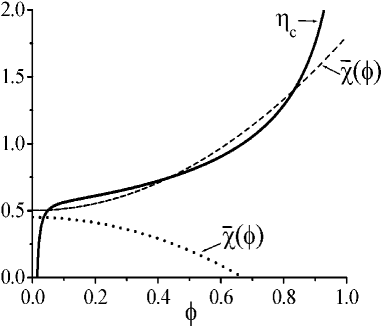
FIG. 1.: Graphical solution of the equilibrium condition of an isolated coil ($N=300$) depicting the crossing of $\eta_{c}(N,\phi)$, as given by (22) with $\overline{\chi}(\phi)$. The two curves cross once when $\overline{\chi}(\phi)$ decreases with $\phi$ (dots) but three intersections, indicating a first order phase transition, may occur when $\overline{\chi}(\phi)$ increases with $\phi$ (dashes).

When the $\phi$ dependence of $\chi$ is overlooked it is convenient to obtain $g_{B}$ in terms of a perturbative parameter $\zeta$ measuring the relative importance of the repulsive binary interactions as compared to an elastic energy of order $kT$. Within this approach $g_{B}$ corresponds to $\zeta=1$.[2] This approach can not however account for the contribution of $T$ dependent higher order terms.

An analytical solution of $\partial F_{el}/\partial R=\pi_{\infty}R^{2}$ for arbitrary $\overline{\chi}(\phi)$ is not feasible. Yet, one may gain insight concerning the swelling and collapse behavior from the general features of the graphical solution of the equilibrium condition. Neglecting numerical factors $\partial F_{el}/\partial R=\pi_{\infty}R^{2}$ can be written as

$$\overline{\chi}(\phi) \approx -\frac{\ln(1-\phi)+\phi}{\phi^{2}}+$$ (22)

$$\frac{1}{N^{2/3}\phi^{1/3}}-\frac{1}{N^{4/3}\phi^{5/3}}\equiv\eta_{c}(\phi,N)$$

The equilibrium states correspond to the intersections of $\overline{\chi}(\phi)$ and $\eta_{c}(\phi,N)$ (Figure 1). When $\chi_{eff}(\phi)=\overline{\chi}(\phi)=\chi$ the two curves intersect at one point only. This is also the case when $\overline{\chi}(\phi)$ is a decreasing function of $\phi$. However, in this situation the intersection occurs at lower $\phi$ in comparison to the intersection between $\eta_{c}(\phi,N)$ and $\overline{\chi}(\phi)=\chi_{0}$ thus indicating stronger swelling. When $\overline{\chi}(\phi)$ is an increasing function of $\phi$ it is possible to distinguish between two important scenarios: (i) $\overline{\chi}(\phi)$ and $\eta_{c}(\phi)$ intersect at a single point. In comparison to the intersection of $\eta_{c}(\phi,N)$ and $\overline{\chi}(\phi)=\chi_{0}$, this occurs at higher $\phi$ thus indicating weaker swelling. (ii) $\overline{\chi}(\phi)$ and $\eta_{c}(\phi)$ intersect at three points. This case corresponds to a $F_{chain}$ (15) exhibiting two minima separated by a maximum thus indicating a collapse taking place as a first order phase transition. Note that this last scenario occurs only for $\overline{\chi}(\phi)$ that increases with $\phi$. Arguing that higher $\overline{\chi}(\phi)$ values indicate a poorer solvent allows for a simple interpretation of this result. When $R$ shrinks, $\phi$ increases leading to a higher $\overline{\chi}(\phi)$. Accordingly, the effective solvent quality diminishes with $R$ thus giving rise to cooperativity leading to a first-order collapse transition. At this point it is important to stress the limitations of the Flory approach as described above. Since the monomer volume fraction, $\phi$, is assumed to be uniform, this model does not allow for the possibility of radial phase separation within a single globule. To investigate such scenarios it is necessary to utilize the Lifshitz theory of collapse.[28] This however is beyond the scope of this work.

While the character of the collapse transition within the Flory approximation is affected by the $\phi$ dependence of $\chi_{eff}$, there is essentially no change in span of the collapsed chain as specified by the condition $\pi_{\infty}=0$. When $\chi(T)$ is independent of $\phi$ and $\phi\ll 1$ this condition leads to $v\phi^{2}\sim\phi^{3}$ and to $R/a\sim|v|^{-1/3}N^{1/3}$. For concentration dependent $\chi_{eff}(T,\phi)$, $\pi_{\infty}a^{3}/kT\approx\frac{1}{2}(1-2\overline{\chi}_{0})\phi^{2}+(\frac{1}{3}-\overline{\chi}_{1}\phi^{3})=0$, leads to

$$\frac{R}{a}\approx\left(\frac{\frac{1}{3}-\overline{\chi}_{1}}{\overline{\chi}_{0}-\frac{1}{2}}\right)^{1/3}N^{1/3}$$ (23)

Thus $R\sim N^{1/3}$ is retained but with a modified numerical prefactor and an additional $T$ dependence introduced by $\overline{\chi}_{1}$.

IV Brushes – Swelling and Collapse within the Alexander Approximation with $\chi_{eff}(\phi)$

The swelling behavior of a brush within the Alexander model exhibits similar trends to those found in the case of the isolated coil. In a good solvent, when $\phi\ll 1$ and $R>N^{1/2}a$, the equilibrium condition for the brush, $\partial F_{el}/\partial R\approx\pi_{\infty}\sigma$, leads to $R/Na^{2}\approx\left(\pi_{\infty}/kT\right)\sigma$ or $R/a\approx N(\pi_{\infty}a^{3}/kT)(\sigma/a^{2})$. As in the case of the coil, the “nearly good solvent” case involves two regimes. The cross-over occurs at

$$\sigma_{B}\approx r_{B}^{2}\approx\left(\frac{1}{3}-\overline{\chi}_{1}\right)^{1/4}g_{B}a^{2}$$ (24)

When $\sigma>\sigma_{B}$ the chains in the brush exhibit self-avoidance and $R/a\approx N\left(a^{2}/\sigma\right)^{1/3}$ while for $\sigma<\sigma_{B}$ one obtains $R/a\approx N\left(a^{2}/\sigma\right)^{1/2}$ corresponding to a brush of ideal chains.

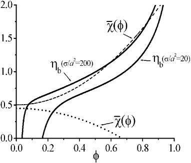
FIG. 2.: Graphical solution of the equilibrium condition of a brush ($N=300$) depicting the crossing of $\eta_{b}(N,\phi,\sigma)$, as given by (27) with $\overline{\chi}(\phi)$. The two curves cross once when $\overline{\chi}(\phi)$ decreases with $\phi$ (dots) but three intersections, indicating a first order phase transition, may occur when $\overline{\chi}(\phi)$ increases with $\phi$ (dashes).

As in the case of a collapsed globule, the thickness of the fully collapsed brush is essentially unaffected by the $\phi$ dependence of $\chi_{eff}$. The thickness is determined by $\pi_{\infty}=0$ but with $\phi\approx Na^{3}/\sigma R$ rather than $\phi\approx Na^{3}/R^{3}$ leading to

$$\frac{R}{a}\approx\left(\frac{\frac{1}{3}-\overline{\chi}_{1}}{\overline{\chi}_{0}-\frac{1}{2}}\right)N\frac{a^{2}}{\sigma}.$$ (25)

that is, the $R\sim N(a^{2}/\sigma)$ scaling is retained with a modified prefactor and an additional $T$ dependence due to $\chi_{1}$.

Again, an analytical solution of $\partial F_{el}/\partial R=\pi_{\infty}\sigma$ for arbitrary $\overline{\chi}(\phi)$ is not practical but it is of interest to consider the graphical solution of the equilibrium condition $\partial F_{el}/\partial R=\pi_{\infty}\sigma$ expressed as

$$\overline{\chi}(\phi) \approx -\frac{\ln(1-\phi)+\phi}{\phi^{2}}-$$ (27)

$$\frac{1}{\phi^{3}}\left(\frac{a^{2}}{\sigma}\right)^{2}+\frac{\phi}{N^{2}}\left(\frac{\sigma}{a^{2}}\right)^{2}\equiv\eta_{b}(\phi,N,\sigma)$$

The equilibrium state is specified by the intersections of $\overline{\chi}(\phi)$ and $\eta_{b}(\phi,N,\sigma)$ (Figure 2). When $\chi_{eff}(\phi)=\overline{\chi}(\phi)=\chi$ the two curves intersect at one point. Similar behavior is found when $\overline{\chi}(\phi)$ is a decreasing function of $\phi$. In comparison to the intersection between $\eta_{b}(\phi,\sigma)$ and $\overline{\chi}(\phi)=\overline{\chi}_{0}$ the intersection occurs at lower $\phi$ thus signaling stronger swelling. As in the case of the coil, it is possible to distinguish between two important scenarios when $\overline{\chi}(\phi)$ increases with $\phi$: (i) $\overline{\chi}(\phi)$ and $\eta_{b}(\phi,N,\sigma)$ intersect at a single point. This occurs at higher $\phi$ in comparison to the intersection of $\eta_{b}(\phi,N)$ and $\overline{\chi}(\phi)=\overline{\chi}_{0}$ and corresponds to weaker swelling. (ii) $\overline{\chi}(\phi)$ and $\eta_{b}(\phi,N,\sigma)$ intersect at three points. In this case $F_{chain}$ exhibits two minima separated by a maximum and the collapse takes place as a first-order phase transition. As we shall discuss shortly, a first order “collapse transition” is indeed possible when $\overline{\chi}(\phi)$ increases with $\phi$. However, this transition involves a vertical phase separation within the brush. To properly analyze this case it is necessary to allow for the spatial variation of $\phi$ thus requiring a more refined description of the brush. This topic is addressed in the next section.

V Brushes – Swelling and Collapse within the Pincus Approximation with $\chi_{eff}(\phi)$

The discussion of the two preceding sections concerned the “global” solvent quality in systems of assumed uniform density. To explore the coupling of the “local” solvent quality with a spatially varying $\phi$ we reanalyze the swelling behavior of a brush using the Pincus approximation instead of the Alexander model. The Alexander model invokes two assumptions: (i) uniform density that is, $\phi$ behaves as a step function thus endowing the brush with a sharp boundary. (ii) The chains are uniformly stretched with their ends straddling the sharp boundary of the brush. While this approximation allows to recover the correct scaling behavior of the brush, the two underlying assumption are in fact wrong. Both $\phi$ and the local extension of the chains vary with the distance from the grafting surface, $z$, and the chain ends are distributed throughout the layer. The Self Consistent Field (SCF) theory of brushes furnishes a rigorous description of these features.[29, 30] The SCF theory provides a basis for the analysis of the coupling of $\chi_{eff}(\phi)$ and $\phi(z)$. Indeed, such analysis was already carried out for the special case of brushes described by the $n$-cluster model. In the following we will use a simpler scheme proposed by Pincus.[17, 21] The level of this approximation is roughly midway between the Alexander model and the SCF theory. It retains the uniform stretching assumption but allows for spatial variation in $\phi$ and in the distribution of the ends. Within this approach the free energy per unit area of the brush is $\gamma=a^{-3}\int_{0}^{R}f_{brush}dz$, where $f_{brush}$ is the corresponding free energy density

$$\frac{f_{brush}}{kT}=\frac{f_{\infty}}{kT}+\frac{z^{2}}{Na^{2}}\Psi(z)-\lambda\phi(z)$$ (28)

The second term allows for the elastic free energy of the chains. A chain having an end at altitude $z$ is assumed to be uniformly stretched and is thus allocated an elastic penalty of $F_{el}/kT\approx z^{2}/Na^{2}$. The chains’ ends are assumed to be distributed throughout the layer with a volume fraction $\Psi(z)$.

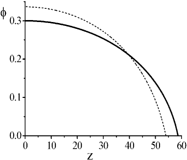
FIG. 3.: The concentration profile, $\phi$ vs. $z$ plots, for a brush of polystyrene in toluene with $N=300$, $\sigma/a^{2}=22.5$ ($\sigma/R_{F}^{2}=0.024$) $T=25^{0}C$ calculated using $\overline{\chi}(\phi)=0.431-0.311\phi-0.036\phi^{2}$.[5] The dashed line depicts the case $\overline{\chi}(\phi)=\overline{\chi}_{0}$ while the continuous line describes $\phi(z)$ for the full $\overline{\chi}(\phi)$.

The core of the Pincus approximation is the assumption that local concentration of ends scales as the fraction of ends within the chain, $1/N$, that is

$$\Psi(z)=\frac{\phi(z)}{N}$$ (29)

As opposed to the SCF theory, $\Psi(z)$ is assumed and not derived. While $\Psi(z)$ is wrong for small altitudes the approximation yield the correct $\phi(z)$ because $F_{el}\approx z^{2}$ and the large $z$ contribution, where the assumed $\Psi(z)$ is reasonable, dominates. Finally, $\lambda$ is a Lagrange parameter fixing the number of monomers per chain, $N$.

The equilibrium concentration profile $\phi(z)$ is specified by the condition $\delta\gamma/\delta\phi=0$. Since $f_{brush}$ does not depend on $d\phi/dz$ the equilibrium condition is $\delta\gamma/\delta\phi=\partial f_{brush}/\partial\phi=0$ or

$$\mu_{\infty}(\phi)/kT=\lambda-Bz^{2},$$ (30)

Here $\mu_{\infty}=\partial f_{\infty}/\partial\phi$ is the exchange chemical potential as obtained from (8)[31]

$$\mu_{\infty}(\phi)/kT=-\ln(1-\phi)-1+\chi_{eff}(\phi)\left(1-\phi\right)-\phi\overline{\chi}(\phi).$$ (31)

In the following we utilize $B=3\pi^{2}/8N^{2}a^{2}$, as obtained from the SCF theory, rather than the value obtained from the Pincus model. Upon making this substitution, equation (30) is identical to the one obtained from the rigorous SCF theory. In the following we impose the condition $\phi_{R}\equiv\phi(R)=0$. This condition is sufficient for our discussion since we are interested in the case of a vertical phase separation within a brush due to a “second type” of phase separation involving coexistence of two phases of finite concentration.

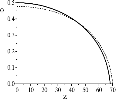
FIG. 4.: The concentration profile, $\phi$ vs. $z$ plots, for a brush of PEO in water with $N=300$, $\sigma/a^{2}=11$ ($\sigma/R_{F}^{2}=0.012$), $T=68^{0}C$ calculated using $\overline{\chi}(\phi)=0.469+$ $0.060\phi-0.241\phi^{2}+0.370\phi^{3}+0.579\phi^{4}$ obtained by polynomial fit of the $\overline{\chi}(\phi)$ data in Ref [6]. The dashed line depicts the case $\overline{\chi}(\phi)=\chi_{0}$ while the continuous line describes $\phi(z)$ for the full $\overline{\chi}(\phi)$.

In the general case, the condition $\phi_{R}=0$ is replaced by $\pi_{\infty}(\phi_{R})=0$, thus allowing for a fully collapsed brush where $\phi_{R}>0$. Since in our case $\phi_{R}=0$, equation (30) specifies $\lambda$

$$\lambda=BR^{2}+\mu_{\infty}(0)/kT.$$ (32)

thus enabling us to rewrite (30) as

$$\Delta\mu_{\infty}(\phi)/kT=B(R^{2}-z^{2})$$ (33)

where $\Delta\mu_{\infty}(\phi)\equiv\mu_{\infty}(\phi)-\mu_{\infty}(0)$ or $\Delta\mu_{\infty}(\phi)/kT=\mu_{\infty}(\phi)/kT+1-\chi_{eff}(0)$. Equation (33) determines the height $R$ of the brush for a given $\phi(z=0)\equiv\phi_{0}$

$$R=\sqrt{\Delta\mu_{\infty}(\phi_{0})/BkT}$$ (34)

and the concentration profile in the form

$$z(\phi)=\sqrt{\left[\Delta\mu_{\infty}(\phi_{0})-\Delta\mu_{\infty}(\phi)\right]/BkT.}$$ (35)

The grafting density corresponding to $\phi_{0}$ is then specified by the constraint

$$\frac{Na^{3}}{\sigma}=\int_{0}^{R}\phi(z)dz$$ (36)

When $\chi(T)$ and $f_{\infty}$ is approximated by $f_{\infty}\approx v(T)\phi^{2}$ the concentration profile of the brush is parabolic. Upon replacing $\chi(T)$ by $\chi_{eff}(T,\phi)$ the concentration profile of the brush $\phi(z)$ is modified because the solvent quality varies, in effect, with the altitude $z$.

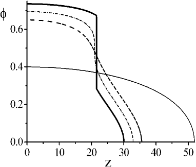
FIG. 5.: $\phi$ vs. $z$ plots, for brushes with $N=300$, $\sigma/a^{2}=18$ ($\sigma/R_{F}^{2}=0.019$) subject to interactions described by $\overline{\chi}(\phi)=0.5$ (thin line), $\overline{\chi}(\phi)=0.5+$ $0.95\phi^{2}$ (dashes), $\overline{\chi}(\phi)=0.5+$ $1.00\phi^{2}$(dash-dots), $\overline{\chi}(\phi)=0.5+$ $1.05\phi^{2}$ (thick line).

As a result, $\phi(z)$ is no longer parabolic. Three principle scenarios are possible. When $\overline{\chi}(\phi)$ is a decreasing function of $\phi$ the brush height, $R$, increases while the concentration at the grafting surface, $\phi_{0}$, decreases. Such behavior is expected, for example, for brushes of polystyrene in toluene (Figure 3). When $\overline{\chi}(\phi)$ is an increasing function of $\phi$ two scenarios are of interest. When there is no phase separation of the second type, the qualitative features of $\phi(z)$ are not modified. However, the brush height, $R$ decreases while the concentration at the grafting surface, $\phi_{0}$ increases. Such is the case for polyetheleneoxide (PEO) brushes in water (Figure 4). A qualitatively different scenario occurs when a second type of phase separation occurs within the brush leading to a discontinuity in $\phi(z)$. This case was first discussed by Wagner et al in the context of the n-cluster model.[20, 21] When $\overline{\chi}(\phi)$ increases with $\phi$ to the extent that a bulk phase separation of the second type occurs it is possible to distinguish between two regimes. For grafting densities lower than $\sigma_{c}$, to be specified below, $\phi_{0}<\phi_{-}$. In this range $\phi(z)<\phi_{-}$ at all altitudes and there is no phase separation. On the other hand, when $\sigma>\sigma_{c}$ phase separation occurs within the brush leading to a discontinuous $\phi(z)$.

The onset of phase separation within the brush for $\sigma>\sigma_{c}$ is signalled by the appearance of multiple roots to equation (35). These are due to the van der Waals loop traced by $\mu_{\infty}(\phi)$ in the range $\phi_{-}<\phi<\phi_{+}$. The corresponding concave region in $f_{\infty}$ gives rise to an unstable domain in $f_{brush}$. The coexistence within the brush is specified by two conditions: (i) $\mu_{brush}(\phi_{+})=\mu_{brush}(\phi_{-})$ where $\mu_{brush}(\phi(z))=\partial f_{brush}/\partial\phi$ is the total exchange chemical potential at $z$, allowing for both the interaction free energy and the elastic one. This leads to $\mu_{\infty}(\phi_{+})/kT-Bz_{+}^{2}=\mu_{\infty}(\phi_{-})/kT-Bz_{-}^{2}$.

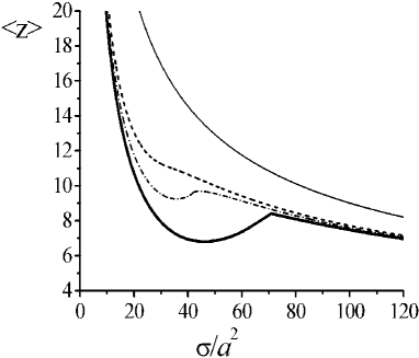
FIG. 6.: $\langle z\rangle$ vs. $\sigma$ plots for brushes with $N=300$ subject to interactions described by $\overline{\chi}(\phi)=0.5$ (thin line), $\overline{\chi}(\phi)=0.5+0.95\phi^{2}$(dashes), $\overline{\chi}(\phi)=0.5+1.00\phi^{2}$(dash-dots), $\overline{\chi}(\phi)=0.5+1.05\phi^{2}$(thick line).

At the phase boundary $z_{+}=z_{-}=R_{i}$ and thus $\mu_{\infty}(\phi_{+})=\mu_{\infty}(\phi_{-})$; (ii) $\pi_{brush}(\phi_{+})=\pi_{brush}(\phi_{-})$ where $\pi_{brush}=\phi^{2}\left[\partial(f_{brush}/\phi)/\partial\phi\right]$ is the local osmotic pressure. Within the Pincus model, this condition clearly reduces to $\pi_{\infty}(\phi_{+})=\pi_{\infty}(\phi_{-})$. Thus, the two coexisting phases are characterized by the monomer volume fractions, $\phi_{+}$ and $\phi_{-}$, of the bulk phases in the $N\rightarrow\infty$ limit. However, because of (33) the coexistence occurs at a single altitude $z=R_{i}$ specified by

$$\Delta\mu_{\infty}(\phi_{\pm})/kT=B(R^{2}-z_{i}^{2})$$ (37)

thus leading to a discontinuity in $\phi(z)$. Clearly, the critical point for this transition, as determined by $\partial^{2}\gamma/\partial\phi^{2}=\partial^{3}\gamma/\partial\phi^{3}=0$, is identical to that of the bulk transition as given by $\partial^{2}f_{\infty}(\phi)/\partial\phi^{2}=0$ and $\partial^{3}f_{\infty}(\phi)/\partial\phi^{3}=0$.

Two approaches allow to explicitly calculate $\phi(z)$ when $\sigma>\sigma_{c}$. In one, the concentration profile is obtained from (35) for the intervals $\phi_{0}\geq\phi\geq\phi_{+}$ and $\phi_{-}\geq\phi\geq 0$. To follow this route it is necessary to first obtain the bulk binodal by utilizing, for example, the Maxwell equal-area construction on the van der Waals loop traced by $\mu_{\infty}(\phi)$.[32] The second approach utilizes a Maxwell construction on the van der Waals loops occurring in the plots of $\phi(z)$ vs. $z^{2}$.[20] It is equivalent to the first route because $z^{2}$ is related to $\mu_{\infty}(\phi)$ via (33).

A vertical phase separation as discussed above becomes possible once $\phi_{0}$ exceeds $\phi_{-}$. To estimate the threshold grafting density necessary, $\sigma_{c}$ we assume that for $\sigma<\sigma_{c}$ the brush thickness retains the scaling behavior of a single phase brush as obtained from the Alexander model and the SCF theory. For a Gaussian brush $R/a\approx N\left(a^{2}/\sigma\right)^{1/2}$ while a brush exhibiting self avoidance obeys $R/a\approx N\left(a^{2}/\sigma\right)^{1/3}$. Since $\Delta\mu_{\infty}(\phi_{0})/kT=BR^{2}$ this leads to $\sigma_{c}\approx\left[\Delta\mu_{\infty}(\phi_{-})/kT\right]^{-3/2}$ in the self-avoidance case and to $\sigma_{c}\approx\left[\Delta\mu_{\infty}(\phi_{-})/kT\right]^{-1}$ for the Gaussian one. This estimates can serve as guidelines when $\Delta\mu_{\infty}(\phi_{0})$ is known, that is when $\overline{\chi}(\phi)$ is available. When this is not the case one may roughly estimate $\sigma_{c}$ by further assuming that the brush is sufficiently dilute to ensure $\Delta\mu_{\infty}(\phi)\sim\phi$ thus leading to

$$\sigma_{c}\approx\left\{\begin{array}[]{l}\phi_{-}^{-3/2}\qquad\text{ self-avoidance}\\ \phi_{-}^{-1}\qquad\text{ Gaussian}\end{array}\right.$$ (38)

This last form is of interest because it permits a crude estimate of $\sigma_{c}$ on the basis of the phase diagram even when $\overline{\chi}(\phi)$ is unknown.

The predicted discontinuity in $\phi(z)$ may prove difficult to resolve experimentally. A more robust signature of the vertical phase separation concerns the dependence of the brush thickness on the grafting density. The vertical phase separation results in non-monotonous dependence of the moments of the profile on $\sigma$. For brevity we consider only the first moment of $\phi(z)$

$$\langle z\rangle=\frac{\int_{0}^{R}z\phi(z)dz}{\int_{0}^{R}\phi(z)dz}=\frac{\sigma}{Na^{3}}\int_{0}^{R}z\phi(z)dz$$ (39)

and illustrate its $\sigma$ dependence for the hypothetical case considered in section II, that is of $\overline{\chi}(\phi)=1/2+\overline{\chi}_{2}\phi^{2}$. In this case the critical point is specified by $\overline{\chi}_{2c}=1$ and $\phi_{c}=1/2$ so that phase separation occurs when $\overline{\chi}_{2}\geqslant\overline{\chi}_{2c}$ and $\phi>\phi_{c}$.

Representative $\phi(z)$ curves for $\overline{\chi}(\phi)$: $\overline{\chi}(\phi)=1/2$, $\overline{\chi}(\phi)=1/2+0.95\phi^{2}$, $\overline{\chi}(\phi)=1/2+\phi^{2}$ and $\overline{\chi}(\phi)=1/2+1.05\phi^{2}$ are depicted in Figure 5. The corresponding $\langle z\rangle$ vs. $\sigma$ plots are shown in Figure 6. The $\langle z\rangle$ vs. $\sigma$ curves exhibit a pronounced minimum when the brush undergoes a vertical phase separation while in the single phase state $\langle z\rangle$ increases monotonically with $\sigma$. The behavior of $\langle z\rangle$ vs. $\sigma$ plot reflects the repartition of the monomers between the two phases.

When $\sigma>\sigma_{c}$ an inner dense phase, with the associated discontinuity in $\phi(z)$, appears. As a result, the corresponding increase in the average density within the brush is mostly spent on the formation of this inner phase. The contribution of this denser phase to $\langle z\rangle$ is however weighted by $z$ thus causing the initial decrease in $\langle z\rangle$.

VI An Illustrative Example-The case of PNIPAM

As we have seen, qualitatively novel scenarios for the collapse of isolated coils and for the structure of polymer brushes occur when $\overline{\chi}(\phi)$ increases with $\phi$. This behavior is apparently realized by Poly(N-isopropylacrylamide) (PNIPAM) in water, a system exhibiting a lower critical solution temperature (LCST) around $30^{0}C$. Three items concerning this system are of interest for our discussion.

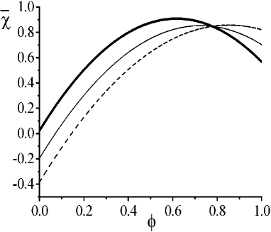
FIG. 7.: A plot of $\overline{\chi}(\phi)$ vs. $\phi$ for PNIPAM as described by the $\chi_{eff}(\phi)$ of Afroze et al.[36, 37] for $T=26^{0}C$ (dash), $T=28^{0}C$ (thin line) and $T=30^{0}C$ (thick line).

First, is an early study by Zhu and Napper[33] of the collapse of PNIPAM brushes grafted to latex particles immersed in water. This revealed a collapse involving two stages. An “early collapse”, took place below $30^{0}C$, at better than “$\theta$-conditions”, and did not result in flocculation of the neutral particles. Upon raising the temperature to worse than “$\theta$-conditions” the collapse induced flocculation. This indicates that the colloidal stabilization imparted by the PNIPAM brushes survives the early collapse. It lead to the interpretation of the effect in terms of a vertical phase separation within the brush due to a second type of phase separation as predicted by the $n$-cluster model. The second item is the experimental study, by Wu and his group, of the collapse behavior of isolated PNIPAM chains.[34] This study concerned dilute aqueous solutions of high molecular weight PNIPAM heated to above the “$\theta$-temperature”. It provided detailed $R$ vs. $T$ plots characterizing the collapse of individual chains. This study was made possible by the apparent decoupling of the collapse and bulk phase separation in the case of PNIPAM. For the present discussion, the conclusion of interest is that the collapse was steeper than expected on the basis of a driving force due to simple binary attractions as modeled by $-v\phi^{2}$ with $v=1-2\chi(T)$. The last item concerns $\chi_{eff}(T,\phi)$ and the phase diagram of PNIPAM. An early study of the phase behavior of PNIPAM in water, by Heskins and Guillet,[35] identified an LCST at $\phi_{c}\simeq 0.16$ and $T_{c}\simeq 31.0^{0}C$. A recent investigation, by Afroze et al.[36] led to different results: (i) While the LCST of PNIPAM depends on $N$ the LCST occurs around $T_{c}\simeq 27-28^{0}C$ and $\phi_{c}\simeq 0.43$ (ii) In the limit of $\phi\rightarrow 0$, the phase separation occurs, depending on $N$, between $30^{0}C$ and $34^{0}C$. Afroze et al than proceeded to obtain $\chi_{eff}(T,\phi)$ assuming that it is well described by $\chi_{eff}(T,\phi)=\sum_{i=0}^{2}\widehat{\chi}_{i}(T)\phi^{i}$ with $\widehat{\chi}_{i}(T)$ of the form $\widehat{\chi}_{i}(T)=A_{i}+B_{i}T$.

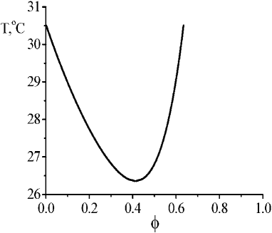
FIG. 8.: The phase diagram of PNIPAM in the limit of $N\rightarrow\infty$ as obtained from the $\chi_{eff}(\phi)$ of Afroze et al.[36, 37]

The six phenomenological parameters were fixed by comparing the theoretical and experimental phase diagrams.[37] In the following we utilize the results of Afroze et al because they are consistent with the results of Zhu and Napper in that they enable a vertical phase separation within a PNIPAM brush below $30^{0}C$.

The items listed above suggest that PNIPAM indeed exhibits the collapse behavior expected when $\overline{\chi}(\phi)$ increases with $\phi$, thus: (i) Zhu and Napper provided evidence for the occurrence of a vertical phase separation within a PNIPAM brush; (ii) Wu and collaborators demonstrated that the collapse of single PNIPAM is observable and that it is steeper than expected thus suggesting $\overline{\chi}(\phi)$ involvement; (iii) The phase diagram measured by Afroze et al permits the interpretation of Zhu and Napper concerning PNIPAM brushes. Furthermore, as we shall see, their $\chi_{eff}(T,\phi)$ yields a $\overline{\chi}(\phi)$ increasing with $\phi$, thus lending further support to (i) and (ii).

The $\overline{\chi}(\phi)$ vs. $\phi$ plots at $T=26^{0}C$, $T=28^{0}C$ and at $T=30^{0}C$, as obtained on the basis of $\chi_{eff}(T,\phi)$ proposed by Afroze et al.[37] (Figure 7) show that $\overline{\chi}(\phi)$ increases with $\phi$. The phase diagram for $N\rightarrow\infty$, (Figure 8) as calculated using this $\chi_{eff}(T,\phi)$, exhibits a second type of phase separation, as stated by Afroze et al. The concentration profiles of a PNIPAM brush, $\phi(z)$ vs. $z$, thus obtained confirm that a vertical phase separation is indeed expected within the brush (Figure 9). The above plots suggest that PNIPAM in water is indeed a system which exhibits the novel signatures associated with $\overline{\chi}(\phi)$ that increases with $\phi$ and with a second type of phase separation. At the same time, it is important to stress that the performance of $\chi_{eff}(T,\phi)$ proposed by Afroze et al. is not faultless. Using this $\chi_{eff}(T,\phi)$ enabled Afroze et al to reproduce satisfactorily only one of the four phase diagrams they studied. With this in mind, the plots in Figures 7–9 should be considered as preliminary.

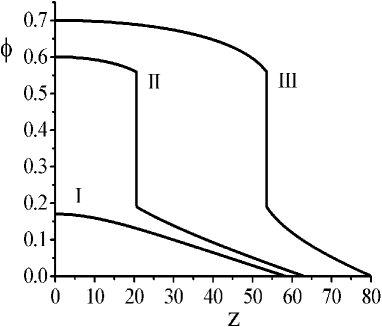
FIG. 9.: $\phi$ vs. $z$ plots for PNIPAM brushes for $N=300$ and $T=28^{0}C$ as obtained from the $\chi_{eff}(\phi)$ of Afroze et al.[36, 37] Curves I, II and III correspond respectively to $\sigma/a^{2}=53$ ($\sigma/R_{F}^{2}=0.056$), $\sigma/a^{2}=19$ ($\sigma/R_{F}^{2}=0.020$), $\sigma/a^{2}=8$ ($\sigma/R_{F}^{2}=0.009$).

Hopefully, better results can be obtained when direct measurements of $\overline{\chi}(T,\phi)$ for PNIPAM in water will become available.

VII Discussion

The necessity of introducing $\chi_{eff}(T,\phi)$ to replace $\chi=\chi(T)$ signals a failure of the Flory free energy. This failure is traceable to deficiencies in the Flory-Huggins lattice model and shortcomings of the approximations invoked in obtaining the Flory free energy. Thus, the Flory-Huggins lattice model assumes that all monomers are identical in size and shape to the solvent molecules. Furthermore, it supposed that all monomers exist in a single state. In turn, the Flory approximation fails to distinguish between monomer-monomer contacts due to intrachain contacts and those due to interchain ones. The resulting free energy is insensitive to the monomer sequence of heteropolymers. It only allows for pairwise attractive interactions and not for higher order attractions involving micelle like clusters of monomers. These deficiencies motivated a number of theoretical refinements of the Flory-Huggins lattice model[9, 22, 23, 38, 39, 40] and of its solution. These refinements are achieved at the price of introducing additional parameters. In certain cases, it is conceivable that a full description of a system may require a combination of a number of these refined treatments. For example, in modelling neutral water soluble polymers it may be necessary to allow for monomer size and shape, the existence of interconverting monomeric states and for the interplay of intrachain and interchain contacts. The number of parameters involved with such a complete description is even higher. With this in mind, it is of interest to utilize a complementary approach involving the Flory free energy and the measured $\overline{\chi}(T,\phi)$, as obtained from the colligative properties of the polymer solutions. In this paper we focused on the relationship between $\overline{\chi}(T,\phi)$, a macroscopic property, and the microscopic swelling and collapse behavior of coils and brushes. As we have seen, this approach yields specific predictions concerning: (i) the cross-over between ideal chain and self avoidance statistics, $g_{B}$; (ii) the concentration profile, $\phi(z)$, of a polymer brush. It also suggests the possibility of a first order collapse transition for flexile chains when $\overline{\chi}(T,\phi)$ increases with $\phi$. This route has the merit of relating independent measurements and helps clarify the significance of $\overline{\chi}(T,\phi)$ and $\chi_{eff}(T,\phi)$ as measures of solvent quality. Clearly, this phenomenological approach does not yield insights concerning the molecular origins of $\overline{\chi}(T,\phi)$ and $\chi_{eff}(T,\phi)$. Consequently, it does not identify molecular design parameters allowing to tune $\overline{\chi}(T,\phi)$ and $\chi_{eff}(T,\phi)$. The applicability of this method is also limited by the paucity of systematic tabulations of $\overline{\chi}(T,\phi)$. To clarify the advantages and disadvantages of this method it is helpful to consider the vertical phase separation within a brush as considered in sections V and VI. In order to design an experiment yielding direct evidence for this transition, it is necessary to identify a polymeric system exhibiting such effect. Another prerequisite is a clear idea of the range of grafting densities, molecular weights and temperatures involved. The effect was originally predicted within the framework of the $n$-cluster model proposed for PEO. This model was subsequently invoked in the interpretation of the indirect evidence for this transition in brushes of PNIPAM. However, utilizing the $n$-cluster model as a guide for further studies is hampered by two problems: (i) the applicability of the $n$-cluster model to this system vis-à-vis the alternative model of Matsuyama and Tanaka[41] is not clear; (ii) the $n$-cluster model, like the competing approach of Matsuyama and Tanaka, invokes parameters that are currently unknown. On the other hand, as we have seen, the necessary information can be obtained directly from experimentally determined $\chi_{eff}(T,\phi)$ (or equivalently, $\overline{\chi}(T,\phi)$). The implementation of this last approach is clearly limited by the accuracy of the reported $\overline{\chi}(T,\phi)$ and $\chi_{eff}(T,\phi)$. This last difficulty, concerning the uncertainties $\overline{\chi}(T,\phi)$ and the phase diagram of PNIPAM, hampers however also the microscopic models that require such data in order to determine the parameters of the theory.

REFERENCES

- [1] Flory, P. J. Principles of Polymer Chemistry Cornell University Press, Ithaca, N.Y. 1953.
- [2] de Gennes, P. -G. Scaling Concepts in Polymer Physics, Cornell University Press, Ithaca, N.Y. 1979.
- [3] Grosberg, A. Yu. ; Khokhlov, A. R. Statistical Physics of Macromolecules, AIP Press, New York, 1994.
- [4] Doi, M. Introduction to Polymer Physics Clarendon Press, Oxford, 1996.
- [5] Schuld, N; Wolf, B. A. Polymer Handbook, 4th ed.; Wiley, NY, 1999.
- [6] Molyneux, P. Water, Franks, F. Ed. Plenum, NY, 1975. Vol 4.
- [7] Huggins, M.L. J.Am. Chem. Soc. 1964, 86,3535.
- [8] In the literature,[5] is sometimes denoted by while denotes . Our notation aims to avoid confusion with the customary usage of .
- [9] (a) de Gennes P.-G. CR Acad. Sci, Paris II 1991, 117, 313 (b) de Gennes P.-G. Simple Views on Condensed Matter, World Scientific, Singapore, 1992.
- [10] Qian, C.; Mumby, S. J.; Eichinger, B.E. Macromolecules 1991, 24, 1655.
- [11] Šolc, K.; Koningsveld, R. J. Phys. Chem. 1992, 96, 4056.
- [12] Schäfer-Soenen, H.; Moerkerke, R.; Berghmans, H.; Koningsveld, R.; Dušek, K.; Šolc, K. Macromolecules 1997, 30, 410.
- [13] Bekiranov, S.; Bruinsma, R.; Pincus, P. Europhys. Lett 1993, 24, 183.
- [14] Jeppesen, C.; Kremer, K. Europhys. Lett. 1996, 34, 563.
- [15] Alexander, S. J. Phys (France) 1977 38, 977.
- [16] Halperin, A.; Tirrell, M.; Lodge, T.P., Adv. Polym. Sci. 1992, 100, 31.
- [17] Pincus, P. Macromolecules, 1991, 24, 2912.
- [18] Safran, S. Statistical Thermodynamics of Surfaces and Interfaces, Addison-Wesley, New-York, 1994
- [19] For brevity we will often replace and by and .
- [20] Wagner, M.; Brochard-Wyart, F.; Hervet, H.; de Gennes, P.-G. Colloid Polym. Sci. 1993, 271, 621.
- [21] Halperin, A. Eur. Phys. J. B 1998, 3, 359.
- [22] (a) Foreman, K.W.; Freed, K. F. Adv. Chem. Phys. 1998, 103, 335. (b) Li, W.; Freed, K. F.; Nemirovsky, A. M. J. Chem. Phys. 1993, 98, 8469.
- [23] Painter, P. C.; Berg, L. P.; Veytsman, B.; Coleman, M. M. Macrmolecules 1997, 30, 7529.
- [24] Borisov, O.V.; Halperin, A. Macromolecules 1999, 32, 5097.
- [25] Baulin, V.; Halperin, A. Macromolecules (in press)
- [26] is obtained by integrating .
- [27] The choice of is motivated by two considerations: (i) the experimentally reported is often close to (ii) this is the simplest form yielding a second type of phase separation with . It is useful to compare this form of to that obtained in the -cluster model considered by deGennes, where , and thus leading to and to . Within the -cluster model our choice of is closest to and thus leading to and to . The differences between the two are due to the choice of , in our case vs. as chosen by de Gennes.[9]
- [28] (a) Lifshitz, I.M.; Grosberg, A. Yu. Sov. Phys. JETP 1974, 38, 1198. (b) Lifshitz, I.M.; Grosberg, A. Yu.; Khokhlov, A. R. Rev. Mod. Phys. 1978, 50, 683.
- [29] S.T. Milner, Science, 1991, 251, 905.
- [30] Zhulina E.B.; Borisov O.V.; Pryamitsyn V.A.; Birshtein T.M., Macromolecules,1991, 24,140.
- [31] Upon expressing in terms of we obtain .
- [32] The equality leads to and thus to . Since the binodal is determined by and the equal area construction is specified by .
- [33] (a) Zhu, P.W.; Napper, D. H. J. Colloid Interface Sci. 1994, 164, 489. (b) Zhu, P.W.; Napper, D. H.Colloids Surfaces A 1996, 113, 145.
- [34] (a) Wu, C.; Zhou, S. Macromolecules, 1995, 28, 8381(b) Wu, C.; Wang, X. Phys. Rev. Lett. 1998, 80, 4092.
- [35] Heskins, M.; Gillet, J.E. J. Macromol. Sci. Chem. 1968, A2, 1441.
- [36] Afroze, F.; Nies, E.; Berghmans, H. J. Molecular Structure 2000, 554, 55.
- [37] as obtained by Afroze et al.[36] is specified by , , , , , .
- [38] Matsuyama, A.; Tanaka, F. Phys. Rev. Lett. 1990 , 65, 341.
- [39] Bekiranov, S.; Bruinsma, R.; Pincus, P. Phys. Rev. E 1997, 55, 577.
- [40] Karlstrom, G. J. Phys. Chem. 1985, 89, 4962.
- [41] Matsuyama, A.; Tanaka, F. J. Chem. Phys. 1991, 94, 781.