Exact Hurst exponent and crossover behavior in a limit order market model

Abstract

An exclusion particle model is considered as a highly simplified model of a limit order market. Its price behavior reproduces the well known crossover from over-diffusion (Hurst exponent $H>1/2$) to diffusion ($H=1/2$) when the time horizon is increased, provided that orders are allowed to be canceled. For early times a mapping to the totally asymmetric exclusion process yields the exact result $H=2/3$ which is in good agreement with empirical data. The underlying universality class of the exclusion process suggests some robustness of the exponent with respect to changes in the trading rules. In the crossover regime the Hurst plot has a scaling property where the bulk deposition/cancellation rate is the critical parameter. Analytical results are fully supported by numerical simulations.

PACS numbers: 05.40; 89.90 +n
Keywords: Limit order market, Hurst exponent, KPZ equation, asymmetric exclusion process.

1 Introduction

Financial markets have in recent years been at the focus of physicists attempts to apply existing knowledge from statistical mechanics to economic problems [1, 2, 3, 4]. These markets, though largely varying in details of trading rules and traded goods, are characterized by some generic features of their financial time series, called ‘stylized facts’ [1, 2, 4]. Agent based models of financial markets are successful to reproduce some stylized facts [5, 6, 7, 8, 9, 10], such as volatility clustering, fat-tailed probability distribution of price increments and over-diffusive price behavior at short time scales and diffusive behavior at later times. But all of them need an explicit price formation rule that links excess demand to price changes [11, 5, 12, 13], that can be itself problematic. An other approach consists in modeling the price formation, for instance in limit order markets [14, 15, 16, 17, 18]. So far, all these models of limit order markets have under-diffusive prices at short times, with a crossover to diffusive prices at longer times for some of them. Underdiffusive behavior at short times is realistic in limit order markets, but all these models lack the over-diffusive price behavior observed in real markets at medium time scales. Here, we introduce a crude non-equilibrium model with overdiffusive price that is able to reproduce the crossover from a Hurst exponent $H=2/3$ to $H=1/2$ at larger times, when correlations in the price dynamics are washed out by cancellations of existing orders and independent placements of new orders. In the early time regime our model belongs to the $1d$-KPZ universality class [19], hence, its mechanism for over-diffusive price spreading is robust and analytically tractable.

In section II we define our model in terms of the limit order market dynamics. Our simulation results are presented in section III. In section IV the equivalence of the early-time regime of our model to the totally asymmetric exclusion process (TASEP) [20] with a second class particle is established and its relation to the KPZ [21] and noisy Burgers [22] equation are discussed.

2 Model definition

We consider two types of orders: limit orders that are wishes to buy or sell a given quantity of stock at a given price, and market orders that are orders to immediately sell or buy an asset at the best instantaneous price. Limit orders are stored in an order book until they are either canceled, or fulfilled, provided that the current market price has moved towards their prices. The model is constructed as a one dimensional lattice model, in a similar spirit as in [14, 23]. Let the lattice of length $L$ represent the price axis, with the lowest price on the left end at site 1 and the highest one on the right at site $L$. Limit orders of the two different kinds, i.e., asks ($A$) and bids ($B$) are placed on the lattice according to the price that the order is based on. As bids name lower prices than asks, they will be found on the left side of the lattice. The current market price ($x$) separates the two regions. Sites representing prices at which currently no order is placed are indicated as $0$.

In the model we made the following simplifying assumptions:

• Only one kind of asset is traded and its price dynamics is not directly influenced by outside sources but just by the state of its limit order book.

• Each site can only carry one order (exclusion model).

• Limit orders of either kind come in a unit size.

• Only a finite price interval of width $L$ is considered.

The last assumption is justified as trade only takes place in a narrow interval around the market price. In our model $L$ can be chosen arbitrarily. For a discussion on differences between models and real limit order markets see e.g. [24].

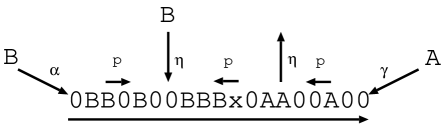
Figure 1: Example of a configuration and possible moves with their assigned rates.

The dynamics of the lattice is as follows (see Figure 1):

• At site $1$ bids enter the system at rate $\alpha$: $0\rightarrow B$.

• At site $L$ asks enter the system at rate $\gamma$. $0\rightarrow A$.

• Asks and bids can diffuse one site towards the market price at rate $p$ provided no other order is already placed at the target site: $B0\rightarrow 0B,\enspace 0A\rightarrow A0$.

• Bids can be placed at unoccupied sites left of the market price at rate $\eta$. The same holds for asks being placed right of the market price: $0\rightarrow A,\enspace 0\rightarrow B$.

• Bids and asks can be evaporated at rate $\eta$: $A\rightarrow 0,\enspace B\rightarrow 0$. This reflects both orders being canceled as well as being timed out. We have made the simplifying assumption of a constant removal rate at each site instead of considering the lifetimes of individual orders.

• An ask can be fulfilled at rate $p$ by an incoming market order, provided it is adjacent to the current market price. Thus the order is removed: $xA\rightarrow 0x$.

• A bid can be fulfilled at the same condition and rate, leading to a decrease of the market price and removal of the order: $Bx\rightarrow x0$.

The role of order injection and diffusion is to ensure a fluctuating order density on both sides of the price. On the other hand, the dynamics of the special particle which represents the price, is such that the sign of price increments is constant as long as the bid-ask spread is not minimal, i.e., as long as the price is not surrounded by two orders. This is a crude but efficient way of implementing trends in limit order market models. Notice that this dynamics implies that the price is always between the best bid and best ask orders, which is true 95% of the time in ISLAND ECN (www.island.com). Even if it is likely that orders do not diffuse [16], we use this ingredient as a way of obtaining exact results for the Hurst exponent.

3 Simulation results

Throughout our simulations we chose initial configurations where each site of the lattice is randomly occupied by an order with probability $1/2$. Furthermore we chose $\alpha=\gamma=1/4$, $p=1/2$. The lattice size $L$ was chosen such that the market price $M$ could not fluctuate out of the represented price interval during the simulation time. The choice of rates guarantees that the price has no drift but on average remains on its initial position, i.e., $L/2$. Averaging over initial conditions is implied in all our simulations.

In the case $\eta=0$ we remain with a model where price dynamics is solely caused by diffusion of limit orders. We are mainly interested in the Hurst exponent $H$ defined by the relationship $\left<(\delta x)^{2}\right>^{1/2}\propto\Delta t^{H}$.

Figure 2: Fluctuations of the price signal $\sqrt{\langle x^{2}(t)\rangle}\propto t^{H}$ at $\eta=0$ and fit with $H=2/3$.

In Fig. 2 we show the fluctuation of the price position $x$ relative to the initial price versus time, in a double-logarithmic plot. As can be seen the Hurst exponent of the model is $H=2/3$ for all times without a crossover. This behavior is in contrast to the corresponding result from the basic Bak, Paczuski, Shubik (BPS) model [14, 23]. In the BPS models offers to buy and sell diffuse on a lattice representing prices just as in our model. The difference is that upon meeting offers to sell and buy mutually annihilate in the BPS model, thus carrying the model to the universality class of the $A+B\rightarrow 0$ reaction diffusion model. For that model it is known analytically that $H=1/4$ at long times plus logarithmic corrections at shorter times [25]. In our model no mutual annihilation (of ask and bid), takes place, but just one type of order vanishes (ask or bid, fulfilled together with a market order), thus causing a price change. This carries our model into the realm of the KPZ universality class as we will illustrate in the next section and yields $H=2/3$.

Figure 3: Correlations of the increments at $\eta=0$ and fit by the eye with a function decaying algebraically as $t^{-1/2}$.

Price increments $\delta x(t)=x(t^{\prime}+t)-x(t^{\prime})$ show algebraically decaying correlations (Figure 3), with $\langle\delta x(t^{\prime})\enspace\delta x(t^{\prime}+t)\rangle\propto t^{-1/2}$ whereas these correlations should be essentially zero; this is due to the absence of evaporation (see below); the correlation of absolute increments has algebraically decreasing autocorrelation with an exponent of approximately 1. These long ranged correlations cause the over-diffusive behavior.

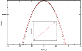
Figure 4: Distribution of the increments (logarithmic scale) for $t=50$ at $\eta=0$ and Gaussian fit. The inset shows the variance of the distribution as a function of time and a fit proportional to $t^{4/3}$.

Due to the price process itself ($|\delta x(1)|\in{0,1}$), the histogram of $\delta x(t)$ is almost Gaussian in shape, the tails appear even less pronounced than a Gaussian pdf (Figure 4). The variance of the distribution of increments $\delta x(t)$ increases as $\sigma\propto t^{4/3}$ (see inset of Figure 4). The dynamical exponent of the price process extracted from this property is $z=3/2$. Clearly the stochastic process causing the price movements is not Gaussian, not even a rescaled Gaussian.

Figure 5: Fluctuations of the price signal $\sqrt{\langle x^{2}(t)\rangle}\propto t^{H}$ at $\eta=1/512$ and fit with $H=2/3$ in the early time regime and $H=1/2$ at late times.

In what follows we consider the case $\eta\neq 0$. Clearly this is more realistic than $\eta=0$ as it is possible to place orders of either kind at any unoccupied site on the price axis without having to perform diffusion steps all the way from the boundaries. Also the withdrawal of orders due to cancellation and timeout becomes thus possible. As seen in Figure 5 the fluctuations of the price signal show a crossover from super-diffusive behavior at short times, characterized by the Hurst exponent $H=2/3$ to diffusive behavior at later times, implying $H=1/2$.

Figure 6: Decay of the correlations of the increments for $\eta=0$ (upper curve) and $\eta=1/8$ (lower curve).

The local random events controlled by the parameter $\eta$ destroy the long ranged time correlations of the price increments. This can be seen in Figure 6, showing the correlation of increments $\langle\delta x(t)\enspace\delta x(0)\rangle$ as a function of $t$ for $\eta=0$ and $\eta=1/8$. At $t=200$ the correlation function for the $\eta=0$ case is still different from zero, while a decay to zero for the other case occurred long since. Note that the autocorrelation of price increments should be negative for short time whereas it is positive in our model; this is due to the fact that we do not allow the coexistence of the two types of markets orders (see [30]).

Figure 7: Fluctuations $\sqrt{\langle x^{2}(t)\rangle}$ for $\eta=1/8$, $\eta=1/32$, $\eta=1/128$ and $\eta=1/512$ (from below). The parameter $\eta$ controls the range over which $H=2/3$ (dashed line).

Adjusting the rate $\eta$ serves as a parameter to control the crossover point. Figure 7 shows the price fluctuations for values of $\eta$ between 1/8 and 1/512. The larger the rate $\eta$ for local events, the shorter is the time span for over-diffusive fluctuations. In fact, in our simulations over-diffusive behavior over a longer time interval appears only to be possible at seemingly meaningless low rates $\eta$, namely $\eta\approx 1/L$, compared to $\alpha=\gamma=1/4$ and $p=1/2$. From the study of empirical data of the Island ECN limit order market conducted in [16] it is known that about 80 per cent of limit orders in the respective market vanished due to timeouts. Only 20 per cent of the offers were (at least partially) fulfilled. We measured these quantities as a function of $\eta$ in our simulations, where fulfillment of an order means either the process $Bx\rightarrow x0$ or $xA\rightarrow 0x$ and timeouts are reflected by the rate $\eta$. It turns out that for a lattice of $L=1000$ at $\eta=1/512$ about 8 per cent of orders were fulfilled and at $\eta=1/1024$ about 16 per cent. Thus the choice of small $\eta$ matching the observed fulfillment rate is realistic and could in fact be used as a means to gauge the simulation time by comparing the known empirical crossover time and the simulation crossover.

In the spirit of dynamical scaling it is tempting to assume that the price fluctuations with sufficiently low $\eta$ can be described in terms of a scaling function $F$ with

$$<x^{2}(t)>=\eta^{-\mu_{1}}F(\eta^{\mu_{2}}t)$$

Since $\eta$ is a rate with inverse dimension of time one expects $\mu_{2}=1$ for covariance of $<x^{2}(t)>$ under rescaling of time. For small times, i.e., small arguments of the scaling function, this ansatz should reproduce the behavior $<x^{2}(t)>\propto t^{4/3}$ which implies $F(y)\propto y^{4/3}$ for $y\to 0$. Independence of $\eta$ thus yields the scaling relation

$$4/3\mu_{2}=\mu_{1}$$ (1)

Hence one expects $\mu_{1}=4/3$. For large times crossover to diffusion implies $F(y)\propto y$ for $y\to\infty$. For large $\eta$ (of order 1 and larger) we obtain ordinary random walk behavior even at early times and the scaling relations are not expected to be valid.

Figure 8: Data collapse for the data for $\eta=1/32$, to $\eta=1/1024$ using the scaling function given in the text and lines to guide the eye corresponding to $H=2/3$ and $H=1/2$.

These arguments are well born out by Monte Carlo simulations. The best fit for the data could be achieved for the choice $\mu_{1}=1.31$ and $\mu_{2}=1.04$. These exponents are used in the plot (Fig. 8). The scaling property suggests that the relevant time scale of the model is $\tau=1/\eta$, which is the average time between successive placements or evaporations of an order at a given site.

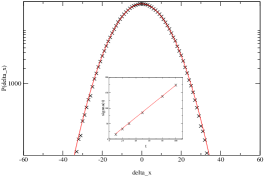
Figure 9: Distribution of the increments for t=50 at $\eta=1/8$ and Gaussian fit. The inset shows the variance of the distribution as a function of time and the linear asymptote.

The increments of the price signal $\delta x(t)$ for $\eta\neq 0$ (Fig. 9) differ from $\eta=0$ in two important respects. Firstly, the tails of the distribution are closer to a Gaussian. A second and more pronounced difference is the behavior of the variance $\sigma$ of the distribution as a function of time, which shows a crossover from $\sigma\propto t^{4/3}$ to $\sigma\propto t$ just as the price signal itself. This means that the price performs an ordinary random walk at long times. A snapshot of the price movement is shown in Figure 10.

Figure 10: Snapshot of price movement at $\eta=1/8$.

4 Connection to the TASEP

The virtue of our model is the equivalence at $\eta=0$ to the totally asymmetric exclusion process (TASEP) for which a wealth of exact results exists [20]. In the TASEP excluding particles enter a lattice at rate $\alpha$ from the left and hop with rate $p$ to the right, provided the target site is empty. At the right end they can leave the system with rate $\beta$. In connection with the TASEP a ’second class’ particle [26] has been defined to have the following dynamics: A first class particle meeting upon a second class particle to its right will exchange places. A second class particle with a vacant right neighboring site hops to that site. The second class particles motion is designed such that it does not interfere with the motion of the first class particles. In fact, the motion of a single second class particle in the system is on average that of a density fluctuation in the system.

Upon coarse graining the dynamics of the TASEP can be described by the noisy Burgers equation, which is closely related to the KPZ equation known to have a universal dynamical exponent $z=3/2$ [19]. This implies a Hurst exponent $H=2/3$ as discussed above. For the noisy Burgers equation the over-diffusive spreading of a density fluctuation (i.e., the spreading of the second class particle, representing the price signal in our model) with $H=2/3$ has been shown analytically [22] in the case of statistically averaging over initial positions as well as realizations, which is always implied in our simulations.

The mapping between our model and the TASEP is as follows: The market price $x$ represents the second class particle. Left of its position, bids are first class particles in the sense of the TASEP and vacancies remain what they are. To the right of the market price vacancies take the role of first class particles in the TASEP sense and asks that of vacancies. The price dynamics in our model is precisely that of a second class particle or density fluctuation in the TASEP.

The TASEP may be seen as a discretized version of the noisy Burgers equation. It is an exactly solvable model for which $z=3/2$ has been obtained through the Bethe ansatz [27]. More recently, also the distribution of the second class particle for averaged random initial conditions has been calculated exactly through a correspondence with statistical properties of random matrices [28]. This confirms the results of our simulations for a finite lattice with open boundaries, but system large enough to be equivalent to an infinite system. We have also performed simulations for a fixed random initial state. We found that the super-diffusive spreading of the second class particle prevails, but the amplitude $<x^{2}>/t^{4/3}$ depends on the initial condition. This is in accordance with expectations [29].

5 Conclusions

In this work we have presented a model exhibiting the empirically observed crossover of the Hurst exponent from $H>1/2$ to $H=1/2$. By a mapping to the totally asymmetric exclusion process we obtain the exact value $H=2/3$ which is close to what is often observed in real markets. The existence of an exact analytic solution puts our model in contrast to the model by Bak [14] exhibiting over-diffusive spreading by volatility feedback into the system and a copying strategy of the traders, but for which no analytical solution is known. The over-diffusive behavior results from time correlations build up in the biased internal motion of asks and bids respectively which together with market orders drive the price process. We identify the average time between evaporation events of orders (due to time-out or cancellation respectively) at a given site as the relevant time scale of the model before crossover to diffusive Gaussian behavior.

References

- [1] R. Mantegna, H. E. Stanley, An Introduction to Econophysics, Cambridge University Press, Cambridge, 2000.
- [2] J.-P. Bouchaud, M.Potters, Theory of Financial Risks, Cambridge University Press, Cambridge, 2000.
- [3] J. D. Farmer, Computing in Science and Engineering, November-December, pp. 26-39 (1999).
- [4] M. M. Dacorogna, R. Gençay, U. Müller, R. B. Olsen, O. V. Pictet, An Introduction to High-Frequency Finance, Academic Press, London, 2001.
- [5] R. Cont, J.-P. Bouchaud, Macroecon. Dyn. 4 (2000), 170.
- [6] T. Lux, M. Marchesi, Nature 397 (1999), 498.
- [7] P. Jefferies, M.L. Hart, P.M. Hui, N.F. Johnson, preprint cond-mat/9910072.
- [8] D. Challet et al., Quant. Fin. 1 (2001), 168. CMZ01.
- [9] D. Challet, M. Marsili, Y.-C. Zhang, Physica A 294 (2001), 514.
- [10] I. Giardina, J.-P. Bouchaud, M. M zard, Physica A 299 (2001), 28.
- [11] J. D. Farmer, Santa Fe Institute working paper 98-12-117.
- [12] P. Jefferies, M.L. Hart, P.M. Hui, N.F. Johnson, Eur. Phys. J. B 20 (2001), 493.
- [13] D. Helbing, D. Kern, Physica A 287 (2000), 259.
- [14] P. Bak, M. Paczuski, M. Shubik, Physica A 246 (1997), 430.
- [15] S. Maslov, Physica A 278 (2000), 571.
- [16] D. Challet, R. Stinchcombe, Physica A 300 (2001), 285.
- [17] M. G. Daniels, J. D. Farmer, G. Iori, E. Smith, cond-mat/0112422.
- [18] J.-P. Bouchaud, M. Mézard, M. Potters, cond-mat/0203511.
- [19] For a review see J. Krug, in: C. Godrèche (Eds.), Solids far from equilibrium, Cambridge University Press, New York, 1991.
- [20] For a review see G. M. Schütz, in: C. Domb, J. Lebowitz (Eds.), Phase Transitions and Critical Phenomena, Vol. 19, Academic, London, 2000.
- [21] M. Kardar, G. Parisi, Y.-C. Zhang, Phys. Rev. Lett. 56 (1986), 889.
- [22] H. van Beijeren, R. Kutner, H. Spohn, Phys. Rev. Lett. 54 (1985), 2026.
- [23] L.-H. Tang, G.-S. Tian, Physica A 264 (1999), 543.
- [24] S. Maslov, M. Mills, Physica A 299 (2001), 234.
- [25] G. T. Barkema, M. J. Howard, J. L. Cardy, Phys. Rev. E 92 (1996), 2017.
- [26] P. A. Ferrari, C. Kipnis, E. Saada, Ann. Prob. 19 (1991), 226.
- [27] L. H. Gwa, H. Spohn, Phys. Rev. Lett. 68 (1992), 725.
- [28] M. Prähofer, H. Spohn, in: V. Sidoravicius (Eds.), In and out of equilibrium, Progress in Probability, Birkhauser, 2002.
- [29] H. Spohn, private communication (2001).
- [30] D. Challet and R. Stinchcombe, in preparation