Relation between Effective Conductivity and Susceptibility of Two – Component Rhombic Checkerboard

Abstract

The heterogeneity of composite leads to the extra charge concentration at the boundaries of different phases that results essentially nonzero effective electric susceptibility. The relation between tensors of effective electric susceptibility $\widehat{\chi}_{ef}$ and effective conductivity $\widehat{\sigma}_{ef}$ of the infinite two–dimensional two–component regular composite with rhombic cells structure has been established. The degrees of electric field singularity at corner points of cells are found by constructing the integral equation for the effective conductivity problem. The limits of weak and strong contrast of partial conductivities $\sigma_{1},\sigma_{2}$ are considered. The results are valid for thin films and cylindrical samples.

I Introduction

The evaluation of effective properties for two–dimensional (2D) two–component composites, which determine the behavior of the medium at large scales, given rise by Keller keller64 and Dykhne dykhne70 , remains a topic of high activity. Among different approaches (variational bounds ber78 ; mil81 ; asymptotic kell87 ; kozlov89 ; numerical hels91 ; network analogue luck91 ; khfel01 ) used to consider this problem, the analytical approach, being classical problem of mathematical physics, is surprisingly very difficult. Exact values of effective parameters are of great interest even though these values are established in idealized models. It seems that explicit formulae are available only as exceptions. Such formulae which solve the field equations were obtained for two–component regular checkerboard with square berd85 , rectangular obnos96 ; milt2001 and triangular obnos99 unit cell using complex–variables analysis. Another technique (integral equations) was used in the recent papers dealt with square ovch00 and triangular ovch02 regular checkerboard.

Almost all these studies were directed towards effective conductivity $\sigma_{ef}$ evaluation despite of important fact that the heterogeneity contributed to the conducting composite some dielectric properties. The homogeneous metal does not possess static dielectric properties (such as electric susceptibility) because only core electrons can contribute there, but their influence is obviously small. However, heterogeneity leads to the extra charge concentration at the boundaries of different phases, which results essentially nonzero effective electric susceptibility $\chi_{ef}$. The implication follows that the relation between the conductivity $\widehat{\sigma}_{ef}$ and susceptibility $\widehat{\chi}_{ef}$ effective tensors must exist.

In the present paper we will consider the regular 2D two–component rhombic checkerboard and derive such relation. This middle–symmetric structure belongs to $p^{\prime}_{c}mm\;$–plane group belov56 and gives rise to anisotropy of $\widehat{\sigma}_{ef}$. In some sense this anisotropic model is more universal than the regular 2D two–component rectangular checkerboard ($c^{\prime}mm\;$–plane group). Really, the effective electric properties are mostly determined by the corner points of the cell, where the electric field is singular kell87 ; kozlov89 . The structure of composite near these points in rhombic checkerboard is governed by arbitrary angular variable.

II Integral Equation

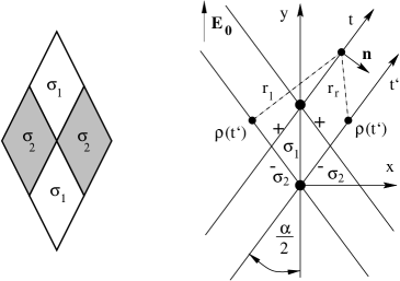
Figure 1: Regular rhombic two – component checkerboard under electric field $E_{0}$: unit cell (left) and basic variables for integral equation (right). The distribution of the charges is drawn in accordance with chosen inequality $\sigma_{1}\geq\sigma_{2}$.

The regular checkerboard structure is composed of rhombic conducting cells with isotropic homogeneous conductivities $\sigma_{1}$ and $\sigma_{2}$, hereafter $\sigma_{1}\geq\sigma_{2}$. The backbone of such structure can be represented as the set of images of the letter ”X” with infinitely long legs, which are shifted up and down to distance $2N\cos{\alpha\over 2}$, $N=0,\pm 1,\pm 2,\ldots$; $\alpha$ is the smallest angle between legs (see Figure 1). The side of the cell is scaled by unit length. Such arrangement of the checkerboard allows to generate the kernel for the integral equation by single series summation rather than by double summation ovch00 ; ovch02 .

We will consider the external unit field $E_{0}$ be applied in vertical direction $Y$. It is one of the principal axes of the effective material tensors. Another axis $X$ may be considered just changing $\alpha\to\pi-\alpha$.

Let us proceed with solution of Laplace equation for a scalar potential $\phi(r)$ at the infinite plane $S$

$$\phi({\bf r})=-E_{0}y-4\pi\int_{S}G({\bf r},{\bf r_{1}})\rho({\bf r_{1}})\;d^{2}r_{1}\;,\;\;\;G({\bf r},{\bf r_{1}})=\frac{1}{2\pi}\ln|{\bf r}-{\bf r_{1}}|\;,$$ (1)

where $G({\bf r},{\bf r_{1}})$ is the two-dimensional Green function and $\rho({\bf r})$ is a charge distribution at the plane. The boundary conditions at the edge relate normal components of the field $E_{n}$ and of the current density $j_{n}$

$$E_{n}^{(1)}-E_{n}^{(2)}=4\pi\rho(t)\;,\;\;\;j_{n}(t)=\sigma_{1}E_{n}^{(1)}=\sigma_{2}E_{n}^{(2)}\;,$$ (2)

where a new variable $t$ is introduced to measure the distance along the edge of a unit cell counted from the cell corner and $\rho(t)$ hereafter is the charge distribution at the edge. The boundary conditions (2) allow to write master equation

$$E_{n}^{(1)}+E_{n}^{(2)}=\frac{4\;\pi}{Z}\rho(r)\;,\;\;\;Z=\frac{\sigma_{1}-\sigma_{2}}{\sigma_{1}+\sigma_{2}}\;,\;\;\;0\leq Z\leq 1\;.$$ (3)

Finding the corresponding derivatives $E_{n}^{(i)}$ (see Appendix A) we come to the integral equation

$$\frac{2\;\pi\;g(t)}{Z}\rho(t)=\sin\frac{\alpha}{2}-4\int_{-\infty}^{+\infty}\rho(t^{\prime})K_{1}(t,t^{\prime})\;dt^{\prime}\;,$$ (4)

where a new function $g(t)$ reflects a periodic interchange of the constituents ($\sigma_{1}$ and $\sigma_{2}$) with variation of argument $t$

$$g(t)=\mbox{sgn[mod}(t,2)-1]\;,\;\;g(-t)=-g(t)\;;\;\;g(t)=-1\;\;\;\mbox{for}\;\;\;0<t\leq 1\;,$$ (5)

the function ${\rm mod}(t,2)$ gives the remainder on division of $t$ by 2 and ${\rm sgn}[x]$ gives -1, 0 or 1 depending on whether $x$ is negative, zero, or positive. The kernel $K_{1}(t,t^{\prime})$ is given by formula

$$K_{1}(t,t^{\prime})=\sum_{k=-\infty}^{+\infty}\left[\frac{k}{(t-t^{\prime})^{2}\tan\frac{\alpha}{2}+(t-t^{\prime}-2k)^{2}\cot\frac{\alpha}{2}}+\frac{k+t^{\prime}}{(t+t^{\prime})^{2}\tan\frac{\alpha}{2}+(t-t^{\prime}-2k)^{2}\cot\frac{\alpha}{2}}\right]$$ (6)

It is worth to represent the kernel for further summation as

$$K_{1}(t,t^{\prime})=\frac{1}{4}\tan\frac{\alpha}{2}\sum_{k=-\infty}^{+\infty}\left[\frac{k}{(k-k_{1})(k-k_{1}^{*})}+\frac{k+t^{\prime}}{(k-k_{2})(k-k_{2}^{*})}\right]\;,$$ (7)

where the zeros $k_{1},k_{1}^{*}$ and $k_{2},k_{2}^{*}$ of both denominators in (6) read

$$k_{1},\;k_{1}^{*}=\frac{t-t^{\prime}}{2}\pm i\;\frac{|t-t^{\prime}|}{2}\tan\frac{\alpha}{2}\;,\;\;\;\;k_{2},\;k_{2}^{*}=\frac{t-t^{\prime}}{2}\pm i\;\frac{|t+t^{\prime}|}{2}\tan\frac{\alpha}{2}\;.$$ (8)

Making use of identity

$$\frac{k+t^{\prime}}{(k-k_{i})(k-k_{i}^{*})}={\rm Im}\left(\frac{k_{i}+t^{\prime}}{k-k_{i}}\right)\frac{1}{{\rm Im}\;k_{i}}\;,$$

we can evaluate (7) in the sense of principal value and reduce essentially the kernel of integral equation (4)

$$K_{1}(t,t^{\prime})=-\frac{\pi}{2}{\rm Im}\left\{\frac{k_{1}\cdot\cot\pi k_{1}}{|t-t^{\prime}|}+\frac{(k_{2}+t^{\prime})\cdot\cot\pi k_{2}}{|t+t^{\prime}|}\right\}\;.$$ (9)

The further simplification of the kernel $K_{1}(t,t^{\prime})$ can be continued by usage of trigonometry. Introducing $\widetilde{\rho}(t)=\rho(t)g(t)$ we obtain finally the integral equation

$$-\frac{2}{Z}\widetilde{\rho}(t)=-\frac{1}{\pi}\sin\frac{\alpha}{2}+\int_{-\infty}^{+\infty}\widetilde{\rho}(t^{\prime})K_{2}(t,t^{\prime})g(t^{\prime})\;dt^{\prime}\;,$$ (10)

where

$$K_{2}(t,t^{\prime})=\frac{\tan\frac{\alpha}{2}\sin\pi(t-t^{\prime})-\sinh\left(\pi(t-t^{\prime})\tan\frac{\alpha}{2}\right)}{\cos\pi(t-t^{\prime})-\cosh\left(\pi(t-t^{\prime})\tan\frac{\alpha}{2}\right)}+\frac{\tan\frac{\alpha}{2}\sin\pi(t-t^{\prime})-\sinh\left(\pi(t+t^{\prime})\tan\frac{\alpha}{2}\right)}{\cos\pi(t-t^{\prime})-\cosh\left(\pi(t+t^{\prime})\tan\frac{\alpha}{2}\right)}$$

The function $\rho(t)$ being a solution of integral equation (10) makes it possible to find an exact expression of the effective conductivity tensor $\widehat{\sigma}_{ef}$ (see Section IV).

III Asymptotic behavior of $\rho(t)$ near the corners

We start this Section with two algebraic properties of the function $\rho(t)$, which will be used in order to simplify further calculation. These are the parity and periodicity of the functions $\widetilde{\rho}(t)$, $\rho(t)$, which are following from (10)

$$\widetilde{\rho}(-t)=\widetilde{\rho}(t)\;,\;\;\;\widetilde{\rho}(t+2)=\widetilde{\rho}(t)\;\;\longrightarrow\;\;\rho(-t)=-\rho(t)\;,\;\;\;\rho(t+2)=\rho(t)\;.$$ (11)

They are in full agreement with physics of the charge distribution $\rho(t)$ along the edges of the cells. A proof follows from an accurate evaluation of integral in (10). Indeed, the parity property follows due to (5) and identity $K_{2}(-t,-t^{\prime})=-K_{2}(t,t^{\prime})$

$$\frac{2}{Z}\widetilde{\rho}(-t)+\frac{1}{\pi}\sin\frac{\alpha}{2}=-\int_{+\infty}^{-\infty}\widetilde{\rho}(-t^{\prime})K_{2}(-t,-t^{\prime})g(-t^{\prime})\;dt^{\prime}=\int_{-\infty}^{+\infty}\widetilde{\rho}(-t^{\prime})K_{2}(t,t^{\prime})g(t^{\prime})\;dt^{\prime}\;.$$ (12)

The periodicity could be proven in the similar way.

A similar integral equation was appeared in Ref. ovch00, for the two – component checkerboard with square unit cell. Its solution is presented by the means of Weierstrass elliptic function $\rho_{sq}(t)\propto{\bf\wp}^{\kappa}(t)$, where $\sin\pi\kappa=Z$, and is found by inspection its behavior near the branch points $t=0$ and $t=1$

$$E_{n}^{(i)}(t)\sim\rho_{sq}(t)\stackrel{{\scriptstyle t\rightarrow 0}}{{\sim}}\frac{1}{t^{2\lambda_{0}}}\;\;,\;\;\;E_{n}^{(i)}(t)\sim\rho_{sq}(t)\stackrel{{\scriptstyle t\rightarrow 1}}{{\sim}}(1-t)^{2\lambda_{1}}\;\;,\;\;\;\lambda_{0}=\lambda_{1}=\kappa\;.$$ (13)

The equality of the exponents $\lambda_{0}=\lambda_{1}$ is here essential. Already the two–component checkerboard with triangle unit cell ovch02 breaks the validity of (13), that made unattainable an explicit solution, but only an efficient approximate method was proposed.

The rhombic structure, discussed in the present paper, also gives rise to distinct exponents. Asymptotic behavior of $\rho(t)$ near the branch points $t=0$ and $t=1$ can be found from the equation (10) (see Appendix A)

$$E_{n}^{(i)}(t)\sim\rho(t)\stackrel{{\scriptstyle t\rightarrow 0}}{{\sim}}\frac{1}{t^{2\mu_{0}}}\; \;\sin\pi\mu_{0}=Z\sin\left[\alpha+\mu_{0}\left(\pi-2\alpha\right)\right]\;,$$ , (14)

$$E_{n}^{(i)}(t)\sim\rho(t)\stackrel{{\scriptstyle t\rightarrow 1}}{{\sim}}(1-t)^{2\mu_{1}}\; \;\sin\pi\mu_{1}=Z\sin\left[\alpha+\mu_{1}\left(2\alpha-\pi\right)\right]\;.$$ , (15)

Then

$$\mu_{0}(Z)=\mu_{1}(Z)=\kappa=\frac{1}{\pi}\arcsin Z\;\;\;\mbox{if}\;\;\;\alpha=\frac{\pi}{2}\;;\;\;\;\;\mu_{0}(Z)=-\mu_{1}(-Z)\;\;\;\mbox{if}\;\;\;\alpha\neq\frac{\pi}{2}\;$$ (16)

and for a large contrast in conductivities $\sigma_{2}\ll\sigma_{1},\;Z\sim 1$: $2\mu_{0}=1,\;2\mu_{1}=\alpha/(\pi-\alpha)$.

This shows that the generic rhombic cell ($\alpha\neq\frac{\pi}{2}$) does not lead to the solution of (10), which can be built out by simple rescaling of Weierstrass elliptic functions. An explicit solution of integral equation remains to be performed.

It turns out that the integral equation (10), obtained in the present Section, is sufficient to establish an exact relation between effective electric conductivity $\widehat{\sigma}_{ef}$ and effective electric susceptibility $\widehat{\chi}_{ef}$, which was not to our knowledge discussed earlier.

IV Effective Susceptibility of Rhombic Checkerboard

Let us consider the polarization of the rhombic checkerboard at the scales large, compared to the size of the cells. The effective electric susceptibility is the tensor which defined by ${\bf P}=\widehat{\chi}_{ef}{\bf E}$ where ${\bf P}$ is polarization and ${\bf E}$ is external electric field. In the reference frame (Figure 1), when $\widehat{\chi}_{ef}$ is diagonalized, its $y$–component is determined by induced dipole moment $d_{y}$ per unit square: $\chi_{ef}^{y}=d_{y}/S$, where

$$d_{y}=\sum_{{\rm over\ all\atop charges\ q_{j}}}y_{j}q_{j}=2\cos{\alpha\over 2}\sum_{k=-\infty}^{\infty}\int_{-\infty}^{\infty}(t+2k)\rho(t)dt$$ (17)

is dipole moment of area $S=L_{x}L_{y}$ and $L_{x},L_{y}$ are the sizes of a sample. The summation covers all induced edge–charges $q_{j}$ which are placed within the area $S$. The sample which is composed of $2N_{x}\times 2N_{y}$ unit cells has the area $S=2N_{x}\;2\sin\frac{\alpha}{2}\times 2N_{y}\;2\cos\frac{\alpha}{2}=8N_{x}N_{y}\sin\alpha$. The formula (17) can be reduced making use of parity and periodicity properties (11) of $\rho(t)$. Its accurate evaluation reads

$$d_{y} = 4N_{y}\cos\frac{\alpha}{2}\int_{-\infty}^{\infty}t\rho(t)dt=4N_{y}\cos\frac{\alpha}{2}\sum_{n=-N_{x}}^{n=N_{x}}\int_{2n-1}^{2n+1}t\rho(t)dt=8N_{x}N_{y}\cos\frac{\alpha}{2}\int_{-1}^{1}t\rho(t)dt\;.$$

Taking into account the inparity (5) of the function $g(t)$ we obtain finally

$$d_{y}=16N_{x}N_{y}\cos\frac{\alpha}{2}\int_{0}^{1}t\widetilde{\rho}(t)dt\;,\;\;\;\;\mbox{and}\;\;\;\;\;\;\chi_{ef}^{y}={1\over\sin{\alpha\over 2}}\int_{0}^{1}t\widetilde{\rho}(t)\;dt\;.$$ (18)

We define also the effective conductivity $\sigma_{ef}$ as a ratio of the current $J=\int j_{n}(t)\;dt$ through the $x$–cross-section of the checkerboard per the unit length to the applied field $E_{0}=1$

$$\sigma_{ef}^{y}=\frac{4\pi}{\sin\frac{\alpha}{2}}\frac{\sigma_{1}\sigma_{2}}{\sigma_{1}-\sigma_{2}}\int_{0}^{1}\widetilde{\rho}(t)\;dt\;,\;\;\;\;\;\sigma_{ef}^{x}(\alpha)=\sigma_{ef}^{y}(\pi-\alpha)\;.$$ (19)

Due to Keller keller64 the principal values of the tensor $\widehat{\sigma}_{ef}$ satisfy the duality relations

$$\sigma_{ef}^{x}(\alpha)\cdot\sigma_{ef}^{y}(\alpha)=\sigma_{1}\sigma_{2}\;.$$ (20)

Relating now two physical quantities (18), (19), we make use of auxiliary integral equation, obtained by integrating the equation (10) (see Appendix B)

$$\frac{\sigma_{2}}{\sigma_{1}-\sigma_{2}}\int_{0}^{1}\widetilde{\rho}(t)\;dt=\frac{1}{4\pi}\sin\frac{\alpha}{2}-\int_{0}^{1}t\;\widetilde{\rho}(t)\;dt\;.$$ (21)

The last relation could be rewritten in new notations (18), (19)

$$4\pi\chi_{ef}^{y}=1-\frac{\sigma_{ef}^{y}}{\sigma_{1}}\;,\;\;\mbox{and similarly}\;\;\;\;4\pi\chi_{ef}^{x}=1-\frac{\sigma_{ef}^{x}}{\sigma_{1}}\;.$$ (22)

One can think that $\sigma_{1}$, which appeared in (22), breaks the universality of the formulae. Actually, the denominator contains the maximal value of partial conductivities $\sigma_{\sf max}=\max(\sigma_{1},\sigma_{2})$.

In fact, we have established the tensorial relation in any reference frame

$$4\pi\widehat{\chi}_{ef}=\widehat{I}-\frac{1}{\sigma_{\sf max}}\;\widehat{\sigma}_{ef}\;,$$ (23)

where $\widehat{I}$ is an identity matrix. Formula (23) results in the particular square–checkerboard case: $4\pi\chi_{ef}^{x}=4\pi\chi_{ef}^{y}=1-\sqrt{\sigma_{2}/\sigma_{1}}$.

Let us consider now two different cases of the weak and large contrast in partial conductivities.

1. $(\sigma_{1}-\sigma_{2})/\sigma_{1}\ll 1$, or $Z\ll 1$:

In the first order on $Z$ the integral equation (10) gives according to definition (19)

$$\rho(t)=-\frac{Z}{2\pi}\sin\frac{\alpha}{2}\;\;\;\longrightarrow\;\;\sigma_{ef}^{x}=\sigma_{ef}^{y}=\sigma_{1}(1-Z)$$ (24)

and therefore

$$4\pi\chi_{ef}^{x}=4\pi\chi_{ef}^{y}=Z\;.$$ (25)

2. $\sigma_{2}\ll\sigma_{1}$:

In this limit the corner points $t\rightarrow 0$ of the cell become important. Making use of the distribution (14) for the fields and charge $E_{n}^{(i)}\sim\widetilde{\rho}(t)\sim t^{-2\mu_{0}}$ one can find approximately in leading terms

$$\mu_{0}=\frac{1}{2}-\frac{1}{\sqrt{\alpha(\pi-\alpha)}}\sqrt{\frac{\sigma_{2}}{\sigma_{1}}}\;\;\;\;\longrightarrow\;\;\sigma_{ef}^{y}=A\;\sqrt{\sigma_{1}\sigma_{2}}\;.$$ (26)

Actually, the coefficient was found in kozlov89 : $A=\sqrt{\alpha/(\pi-\alpha)}\;\cot(\alpha/2)$. Formula (26) implies as well

$$4\pi\chi_{ef}^{x}=1-A\;\sqrt{\frac{\sigma_{2}}{\sigma_{1}}}\;,\;\;\;4\pi\chi_{ef}^{y}=1-\frac{1}{A}\;\sqrt{\frac{\sigma_{2}}{\sigma_{1}}}\;.$$ (27)

V Conclusion

1. We have derived the integral equation for the effective conductivity problem for the regular 2D two–component rhombic checkerboard. An asymptotic behavior of the electric field was investigated near the singular points $t=0$ and $t=1$.

2. The heterogeneity of composite leads to the extra charge concentration at the boundaries of different phases that results essentially nonzero effective electric susceptibility. The exact relation (23) between the two most important electrical properties, namely, effective conductivity $\widehat{\sigma}_{ef}$ and effective susceptibility $\widehat{\chi}_{ef}$, of rhombic composite was established. An absence of specific angular parameter $\alpha$ in this formula make us possible to conjecture its validity for any anisotropic two–component structure. It is shown that the tensor of electrical susceptibility has surprisingly simple structure in both cases of large and small contrast in partial conductivities $\sigma_{1},\sigma_{2}$.

3. The relation derived in present paper is definitely valid for cylindrical samples. It is also valid for thin films due to the conducting nature of the constituents, which confine the electric field inside the conductor.

Appendix A Derivation of integral equation (4). Behavior of its solution near the branch points.

We define the variables

$$x=t\sin\frac{\alpha}{2}\;,\;y=t\cos\frac{\alpha}{2}\;,\;x^{\prime}=\pm t^{\prime}\sin\frac{\alpha}{2}\;,\;\;\;y^{\prime}=t^{\prime}\cos\frac{\alpha}{2}+2k\cos\frac{\alpha}{2}$$ (A1)

and normal vector to the edge

$${\bf n}=\left(\cos\frac{\alpha}{2},-\sin\frac{\alpha}{2}\right)\;.$$ (A2)

Here $k$ is an ordinal number of the ”X” image. Taking in mind the contributions from the both left (l) and right (r) edges of the rhombic tile we will find the derivative $\partial\phi/\partial n=({\bf n}\;\nabla)\;\phi$

$$-\frac{\partial\phi}{\partial n}=E_{0}\sin\frac{\alpha}{2}+\sum_{k=-\infty}^{\infty}\int_{-\infty}^{\infty}dt^{\prime}\rho(t^{\prime})\frac{1}{r_{r}^{2}(t,t^{\prime})}\left(\frac{\partial r_{r}^{2}(t,t^{\prime})}{\partial n}\right)+\sum_{k=-\infty}^{\infty}\int_{-\infty}^{\infty}dt^{\prime}\rho(t^{\prime})\frac{1}{r_{l}^{2}(t,t^{\prime})}\left(\frac{\partial r_{l}^{2}(t,t^{\prime})}{\partial n}\right),$$

which lead after simple algebra to equation

$$\frac{1}{2}\left(E^{(1)}_{n}+E^{(2)}_{n}\right)=-E_{0}\sin\frac{\alpha}{2}+4\int_{-\infty}^{\infty}\rho(t^{\prime})K_{1}(t,t^{\prime})\;dt^{\prime}\;,$$ (A3)

where the kernel $K_{1}(t,t^{\prime})$ reads

$$K_{1}(t,t^{\prime})=\sum_{k=-\infty}^{\infty}\left[\frac{k}{(t-t^{\prime})^{2}\tan\frac{\alpha}{2}+(t-t^{\prime}-2k)^{2}\cot\frac{\alpha}{2}}+\frac{t^{\prime}+k}{(t+t^{\prime})^{2}\tan\frac{\alpha}{2}+(t-t^{\prime}-2k)^{2}\cot\frac{\alpha}{2}}\right]\;.$$ (A4)

Taking now $E_{0}=1$ we arrive at (4).

Below we consider the asymptotic behavior of $\rho(t)$ near the branch points $t=0$ and $t=1$.

• $t\longrightarrow 0$.

Let us assume the power behavior $\rho(t)\propto|t|^{-2\mu_{0}}\cdot\mbox{sgn}\;(t)$ and look for the exponent $\mu_{0}$. The main singularity comes from integral in (10) in the vicinity $t^{\prime}\longrightarrow 0$. The kernel $K_{2}$ behaves as

$$K_{2}(t,t^{\prime})\;\stackrel{{\scriptstyle t,t^{\prime}\rightarrow 0}}{{\longrightarrow}}\;\frac{4}{\pi}\frac{t^{\prime}\tan\frac{\alpha}{2}}{(t-t^{\prime})^{2}+(t+t^{\prime})^{2}\tan^{2}\frac{\alpha}{2}}\;,$$ (A5)

that gives the asymptotic behavior

$$\frac{\rho(t)}{Z}=\frac{1}{\pi}\sin\alpha\int_{-\infty}^{+\infty}\frac{dt^{\prime}\;t^{\prime}\;\rho(t^{\prime})}{t^{2}+(t^{\prime})^{2}-2t\;t^{\prime}\cos\alpha}\;.$$

Defining a new variable $z=t^{\prime}/t$ we obtain

$$\frac{\pi}{Z\sin\alpha}=\int_{0}^{+\infty}\frac{dz\;z^{1-2\mu_{0}}}{1+z^{2}-2z\cos\alpha}+\int_{0}^{+\infty}\frac{dz\;z^{1-2\mu_{0}}}{1+z^{2}+2z\cos\alpha}\;.$$ (A6)

The evaluation of the last expression is based on the primitive fraction expansion with further usage of standard integrals and gives finally (14).

• $t\longrightarrow 1$.

Let us assume the power behavior $\rho(t)\propto|1-t|^{2\mu_{1}}\cdot\mbox{sgn}\;(1-t)$ and look for the exponent $\mu_{1}$. It is convenient to define new variables $\tau=1-t,\;\tau^{\prime}=1+t^{\prime}$ and consider the vicinity of branch point $\tau\rightarrow 0$, so $\rho(t)\propto|\tau|^{2\mu_{1}}\cdot\mbox{sgn}\;(\tau)$. In order to deal with a singular part of the integral equation (10) let us differentiate the last over $t$

$$\frac{2}{Z}\frac{d\;\rho(t)}{dt}=\int_{-\infty}^{+\infty}\rho(t^{\prime})\frac{d\;K_{2}(t,t^{\prime})}{dt}\;dt^{\prime}\;,\;\;\mbox{where}\;\;\;\frac{d\;\rho(t)}{dt}\propto-2\mu_{1}(1-t)^{2\mu_{1}-1}\;.$$ (A7)

The main singularity comes from integral in (A7) in the vicinity $t^{\prime}\rightarrow 1$, or $\tau^{\prime}\rightarrow 0$, where the kernel behaves as

$$\frac{dK_{2}(t,t^{\prime})}{dt}\;\stackrel{{\scriptstyle\tau,\tau^{\prime}\rightarrow 0}}{{\longrightarrow}}\;-\frac{4\sin\alpha}{\pi}\;\frac{\tau^{\prime}(\tau+\tau^{\prime}\cos\alpha)}{(\tau^{2}+(\tau^{\prime})^{2}+2\tau\tau^{\prime}\cos\alpha)^{2}}\;.$$ (A8)

Defining a new variable $v=\tau^{\prime}/\tau$ we obtain

$$\frac{\pi\mu_{1}}{Z\sin\alpha}=\int_{0}^{+\infty}\frac{dv\;v^{2\mu_{1}+1}(1+v\cos\alpha)}{(1+v^{2}+2v\cos\alpha)^{2}}+\int_{0}^{+\infty}\frac{dv\;v^{2\mu_{1}+1}(1-v\cos\alpha)}{(1+v^{2}-2v\cos\alpha)^{2}}\;.$$ (A9)

Evaluating the last integrals we arrive at (15).

Appendix B Derivation of Integral Equation (21)

Reminding that the equation (10) is written in the sense of principal integral value therein, we average this equation at the large interval $[-M,M]$, taking afterward its limit $M\rightarrow\infty$

$$\frac{1}{2M}\int_{-M}^{M}\left[-\frac{2}{Z}\widetilde{\rho}(t)+\frac{1}{\pi}\sin\frac{\alpha}{2}\right]\;dt=\frac{1}{2M}\int_{-M}^{M}dt\int_{-M}^{+M}\widetilde{\rho}(t^{\prime})K_{2}(t,t^{\prime})g(t^{\prime})\;dt^{\prime}\;,$$ (B1)

where due to (11) the left h. s. reads

$$-\frac{2}{Z}\int_{0}^{1}\widetilde{\rho}(t)\;dt+\frac{1}{\pi}\sin\frac{\alpha}{2}$$ (B2)

while the right h. s. could be simplified. Indeed, let us represent the kernel $K_{2}(t,t^{\prime})$ as follows

$$K_{2}(t,t^{\prime}) = \frac{\left(\tan\frac{\alpha}{2}+\cot\frac{\alpha}{2}\right)\sin\pi(t-t^{\prime})}{\cos\pi(t-t^{\prime})-\cosh\left[\pi(t+t^{\prime})\tan\frac{\alpha}{2}\right]}+\frac{\left(\tan\frac{\alpha}{2}+\cot\frac{\alpha}{2}\right)\sin\pi(t-t^{\prime})}{\cos\pi(t-t^{\prime})-\cosh\left[\pi(t-t^{\prime})\tan\frac{\alpha}{2}\right]}+$$ (B3)

$$\frac{1}{\pi}\cot\frac{\alpha}{2}\frac{d}{dt}\ln\left\{\cos\pi(t-t^{\prime})-\cosh\left[\pi(t-t^{\prime})\tan\frac{\alpha}{2}\right]\right\}+$$

$$\frac{1}{\pi}\cot\frac{\alpha}{2}\frac{d}{dt}\ln\left\{\cos\pi(t-t^{\prime})-\cosh\left[\pi(t+t^{\prime})\tan\frac{\alpha}{2}\right]\right\}\;.$$

The last three terms do not contribute to integration of the kernel over $t$, while the first term implies

$$-\frac{2}{Z}\int_{0}^{1}\widetilde{\rho}(t)\;dt+\frac{1}{\pi}\sin\frac{\alpha}{2}=\frac{1}{2M}\int_{-M}^{M}\int_{-M}^{M}\widetilde{\rho}(t^{\prime})K_{3}(t,t^{\prime})g(t^{\prime})\;dt^{\prime}dt\;,$$ (B4)

where

$$K_{3}(t,t^{\prime})=\frac{2}{\sin\alpha}\cdot\frac{\sin\pi t}{\cos\pi t-\cosh\left(\pi(2t^{\prime}+t)\tan\frac{\alpha}{2}\right)}=-\frac{2}{\sin\alpha}\cdot{\rm Re}\left\{\cot\frac{\pi}{2}\left[t+i(2t^{\prime}+t)\tan\frac{\alpha}{2}\right]\right\}\;.$$ (B5)

Continuing the integration of the kernel $K_{3}(t,t^{\prime})$ we notice that the function

$$F(t^{\prime})=\lim_{M\to\infty}\int_{-M}^{+M}K_{3}(t,t^{\prime})\;dt$$ (B6)

is 1–periodic function: $F(t^{\prime}+1)=F(t^{\prime})$, that follows from the structure of the kernel $K_{3}(t,t^{\prime})$. Evaluating the integral in (B6) we arrive at the following

$$F(t^{\prime})=2(1-2t^{\prime})\;\;\mbox{for}\;\;\;0\leq t^{\prime}\leq 1\;.$$ (B7)

The final integral equation

$$2\left(1-\frac{1}{Z}\right)\int_{0}^{1}\widetilde{\rho}(t)\;dt+\frac{1}{\pi}\sin\frac{\alpha}{2}=4\int_{0}^{1}t\;\widetilde{\rho}(t)dt\;$$ (B8)

leads already to (21).

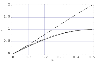
Figure 2: The branch points exponents $\mu_{0}(Z)$ (dashed line) and $\mu_{1}(Z)$ (dot-dashed line) for rhombic unit cell with $\alpha=\pi/3$. The exponent $\kappa(Z)$ (plain line) for square unit cell is also presented.

References

- (1) J. B. Keller, J. Math. Phys., 5, 548 (1964).
- (2) A. M. Dykhne, Sov. Phys. JETP, 32, 63 (1970).
- (3) D. J. Bergman, Phys. Rep. C, 43, 377 (1978).
- (4) G. W. Milton, J. Appl. Phys., 52, 5294 (1981).
- (5) J. B. Keller, J. Math. Phys., 28, 2516 (1987).
- (6) S. M. Kozlov, Russian Math. Survey, 44, 79 (1989).
- (7) J. Helsing, Phys. Rev. B, 44, 11677 (1991); J. Stat. Phys., 90, 1461 (1998).
- (8) J. M. Luck, Phys. Rev. B, 43, 3933 (1991).
- (9) L. G. Fel and K. M. Khanin, J. Stat. Phys., 108, 1015 (2002).
- (10) V. L. Berdichevskii, Vestnik MGU, Math., 40, 15 (1985).
- (11) Y. V. Obnosov, Proc. Roy. Soc. London, Ser. A, 452, 2423 (1996).
- (12) G. W. Milton, J. Math. Phys., 42, 4873 (2001).
- (13) Y. V. Obnosov, SIAM J. Appl. Math., 59, 1267 (1999).
- (14) Y. N. Ovchinnikov and A. M. Dyugaev, Sov. Phys. JETP, 90, 881 (2000).
- (15) Y. N. Ovchinnikov and I. A. Luk’yanchuk, Sov. Phys. JETP, 94 203 (2002).
- (16) N. V. Belov, Kristallografia, 1, 621 (1956).