Measurements of strongly-anisotropic $g$-factors for spins in single quantum states

Abstract

We have measured the full angular dependence, as a function of the direction of magnetic field, for the Zeeman splitting of individual energy states in copper nanoparticles. The $g$-factors for spin splitting are highly anisotropic, with angular variations as large as a factor of five. The angular dependence fits well to ellipsoids. Both the principal-axis directions and $g$-factor magnitudes vary between different energy levels within one nanoparticle. The variations agree quantitatively with random-matrix theory predictions which incorporate spin-orbit coupling.

Strategies for manipulating electron spins are being pursued in many fields[1], from spin-dependent tunneling[2], to magnetic semiconductors[3], to quantum computation[4]. An issue central to all of these fields is that a spin is often not an independent variable. Interactions with the environment, for instance coupling to orbital degrees of freedom, can limit spin coherence times and alter responses to magnetic fields. Here we study the effects of spin-orbit coupling on spins in quantum dots by exploring in detail how the spin properties depend on the direction of an applied magnetic field. Specifically, we measure the $g$-factor for spin Zeeman splitting, the sensitivity with which an energy level shifts with magnetic field. The angular dependence of the $g$-factor has not previously been measured for quantum dots formed from semiconductor 2-dimensional electron gases, because out-of-plane magnetic-field components produce strong orbital effects that make spin energies difficult to observe; we avoid this problem by studying energy levels in copper nanoparticles. We find that the $g$-factors for each quantum state can have striking anisotropies, varying by up to a factor of five depending on field direction. The full dependence on field angle is ellipsoidal, as expected from the tensor properties of the $g$-factor[5, 6]. In addition, the $g$-tensors exhibit large variations between different energy eigenstates in the same nanoparticle, with differences both in the direction of maximum field sensitivity and in magnitude. The variations between levels suggest that the strong anisotropies originate from the intrinsic quantum-mechanical fluctuations of mesoscopic wavefunctions, an effect predicted by random-matrix theories [7, 8].

In bulk systems and for impurities in solids, it is well understood that spin-orbit coupling may cause $g$-factors to exhibit anisotropies associated with directions of the crystal lattice [5, 6]. However, the results of the recent random-matrix-theory work [7, 8] suggest that a different phenomenon may enhance the effects of spin-orbit coupling in nanoscale grains. The idea can be understood by thinking about the wavefunction for an electron in a metal nanoparticle, modeled as an electron in a box with an irregular boundary. The standing wave corresponding to the orbital amplitude of the wavefunction will oscillate strongly and effectively randomly as a function of position, and this complicated wave pattern will vary from quantum state to quantum state. In the presence of spin-orbit coupling, the variations present in the orbital wavefunction are reflected also in the spin properties of an electronic state; in particular, they can cause the $g$-factor to depend on the orientation of an applied magnetic field (${\bf B}$) [7]. The most general dependence on the field direction permitted by symmetry for a spin-$1/2$ particle allows the $g$-factor $g_{\mu}$ for an energy level $\mu$ to be written in the form

$$g_{\mu}(\hat{\bf{B}})=(g_{1}^{2}B_{1}^{2}+g_{2}^{2}B_{2}^{2}+g_{3}^{2}B_{3}^{2})^{1/2}/|\bf{B}|.$$ (1)

where $g_{1}$, $g_{2}$, and $g_{3}$ are the $g$-factors along mutually-orthogonal principal-axis directions (with the convention $g_{1}$ $\geq$ $g_{2}$ $\geq$ $g_{3}$), and $B_{1}$, $B_{2}$, and $B_{3}$ are the magnetic field components in these directions[6, 7]. Pictorially, this means that magnitude of the $g$-factor can be drawn as an ellipsoid. In the absence of spin-orbit coupling, the g-factor for spin splitting should be isotropic. However, in the presence of spin-orbit coupling, random-matrix theory predicts that the three principal-axis g-factors for each level can differ strongly, and the principal-axis directions can vary randomly from energy level to energy level within the same nanoparticle.

We have probed the spin properties of individual quantum states by using electron tunneling to measure energy levels in single copper nanoparticles. We studied in detail two devices containing a nanoparticle with approximately hemispherical shape and a diameter of $\sim$15 nm, based on measured mean level spacings of 0.10 meV (Cu#1) and 0.12 meV (Cu$\#2$). The nanoparticle is connected to two aluminum electrodes by aluminum oxide tunnel junctions, as shown schematically in the inset of Fig. 1. The procedures for fabricating and characterizing the devices have been described in detail previously[9, 10]. We use electron-beam lithography and reactive ion etching to create a 5-10 nm diameter hole in a silicon nitride membrane. A thick Al layer is evaporated on one side of the sample (the bottom side in the inset to Fig. 1) to fill the hole, and then this is oxidized in 50 mT O₂ for three minutes to form an Al₂O₃ tunnel barrier. We form the Cu nanoparticles on top of the membrane by self-assembly during the evaporation of 10 $\AA$ of Cu. The

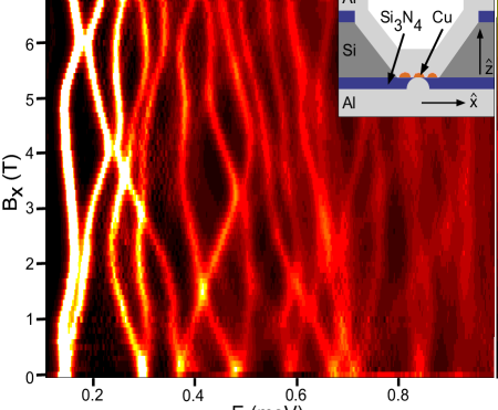
FIG. 1.: Magnetic field dependence of quantum states in copper nanoparticle Cu#1. Main panel: A color-scale plot of the differential conductance ($dI$/$dV$) versus energy ($E$) as a function of magnetic field ($B_{x}$). Yellow corresponds to 2 mS, and black to zero. Values between 2 mS and the maximum conductance of 3 mS are set to white. The energy is equal to the value of source-drain voltage multiplied by the capacitance factor¹² $eC_{1}/(C_{1}+C_{2})=0.66e$. The complex evolution of the levels with $B_{x}$ is due to spin-orbit coupling between spin-up and spin-down quantum states. The inset shows a sample schematic. A small hole in a $Si_{3}$$N_{4}$ membrane is used to make electrical contact to a single copper nanoparticle. $Al_{2}$$O_{3}$ tunnel junctions (not shown) lie between the nanoparticle and aluminum electrodes.

tunnel barrier on top of the nanoparticle is then made by depositing 11 $\AA$ of Al₂O₃ by electron-beam evaporation. Finally, we deposit a thick layer of Al to form the top electrode. We measure current-voltage ($I$-$V$) curves for electrons tunneling from one electrode to the other via the nanoparticle. The measurements are conducted using a dilution refrigerator with an electron base temperature of approximately 40 mK. Once $V$ exceeds a threshold associated with the Coulomb-blockade effect[11], tunneling via the discrete quantum states in the nanoparticle causes the $I$-$V$ curve to take the form of a sequence of small steps, allowing a direct measurement of the spectrum of “electron-in-a-box” states[12].

In Fig. 1 we plot, using a color-scale, differential conductance ($dI/dV$) versus energy ($E$) curves for different values of magnetic field in the x-direction (defined in the Fig. 1 inset), showing how the energy levels in Cu#1 evolve with $B_{x}$. In this figure, $dI/dV$ is obtained by numerical differentiating the $I$-$V$ curves, and the energy is determined by scaling the source-drain voltage to correct for the capacitive division of voltage across the two tunnel junctions in the device[12]. As has been observed previously[10, 12], the energy levels exhibit two-fold Kramers’ degeneracy at $B$=$0$ associated with the electron spin, and they undergo Zeeman splitting as a function of increasing $B$. We determine the $g$-factor from the magnitude of the energy splitting between Zeeman-split states, in the small-$B$ linear regime: $g$=$\Delta$$E(\bf{B})$/($\mu_{B}$$|\bf{B}|$). The data in Fig. 1 exhibit different values of the $g$-factor for different quantum states and a rich variety of avoided level crossings as a function of increasing $B$. The role of spin-orbit coupling in producing these two effects has been discussed previously[10, 13, 14].

Our focus in this letter is the unexplored question of how the $g$-factors for the individual quantum-dot states depend on the direction of the applied magnetic field. We control the field magnitude and direction using a 3-coil magnet which can produce 1 T in any direction, or up to 7 T along one axis[15]. We first verified that the tunneling spectra were identical for $\bf{B}$ and $\bf{-B}$, as expected due to time-reversal symmetry. Thereafter, we took detailed measurements only for $B_{x}$$>$0. For each sample, we measured the Zeeman splitting as a function of $|\bf{B}|$ along 62 different directions selected to span this hemisphere[16]. The values of the $g$-factors showed strong anisotropies, described well by an ellipsoid for each energy level, as demonstrated below. After fitting for the directions of the three principal axes of the $g$-tensor ($\hat{h}_{1}$, $\hat{h}_{2}$, $\hat{h}_{3}$) for each state, we took detailed field scans along these directions to determine precisely the principal-axis $g$-factors, and along arcs of constant field to carefully measure the variation of $g$ with field direction. The long measurement time (1-2 weeks for each sample) requires exceedingly good sample stability.

The directional dependence of $g$ for the first quantum state in sample Cu#1 is shown in Fig. 2. In Fig. 2(a), $dI/dV$ vs. $E$ is plotted as a function of the angle of the magnetic field (with magnitude 700 mT), rotating the field vector around the $\hat{h}_{3}$ principal axis for the first quantum state from an initial orientation along $\hat{h}_{2}$, where $g$ = 0.51$\pm$0.05, to a final orientation along $\hat{h}_{1}$, where $g$ = 0.86$\pm$0.08. The fitted $g$-factors are in good agreement with the form $g(\alpha)=\sqrt{g_{1}^{2}{\rm sin}^{2}(\alpha)+g_{2}^{2}{\rm cos}^{2}(\alpha)}$ expected for an ellipsoid. The data corresponding to a rotation from $\hat{h}_{3}$ (where $g$ = 0.38$\pm$0.05) to $\hat{h}_{1}$ about the $\hat{h}_{2}$ axis are shown in plots (c-d), and for rotation from $\hat{h}_{3}$ to $\hat{h}_{2}$ in (e-f). The $g$-factors along the $\hat{h}_{1}$ and $\hat{h}_{3}$ axes for this quantum state differ by a factor of 2.3. Fig. 2(a) also displays the existence of energy-level to energy-level variations in spin properties. As $\alpha$ increases from 0 to $\pi$/2, the splitting of the first quantum state grows while the splitting of the fourth Zeeman-pair decreases. The other electronic states in Fig. 2 show more complicated behavior due to the alignment of their principal axes in other directions in space. We obtain good fits to ellipsoids for all of the measured states, with the exception of those that undergo an avoided crossing with a neighboring state at a very low value of field, so that the $g$-factor cannot be determined accurately (states 6 and 7 of Cu#1 and states 1, 6, and 7 of Cu#2). The fitted parameters of the measured $g$-factor ellipsoids are listed in Table 1. There are large variations between different

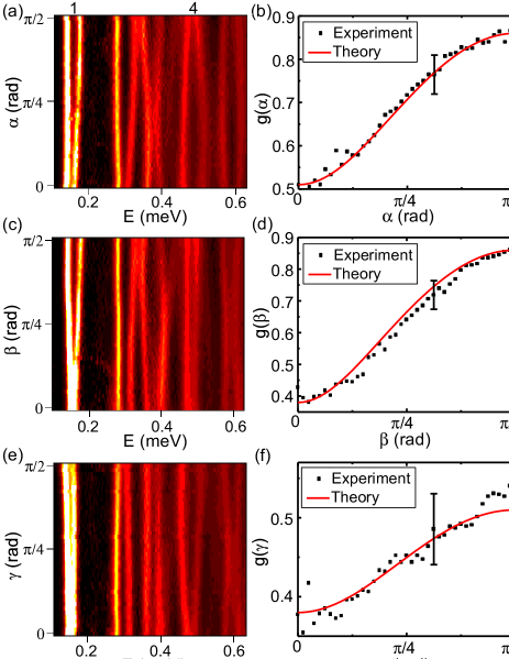
FIG. 2.: Dependence of Zeeman splitting on magnetic-field direction in sample Cu#1. (a), (c), (e) Differential conductance ($dI$/$dV$) as a function of energy ($E$) and the angle of the magnetic field ($\alpha$, $\beta$, or $\gamma$, respectively) for a fixed field magnitude of 700 mT. The data in (a) correspond to a rotation of the field around the $\hat{h}_{3}$ axis for the lowest-energy Zeeman-split energy-level doublet from an initial direction along $\hat{h}_{2}$ to a final direction along $\hat{h}_{1}$, while plots (c) and (e) correspond to rotations from $\hat{h}_{3}$ to $\hat{h}_{1}$ and $\hat{h}_{3}$ to $\hat{h}_{2}$, respectively. The color scale is identical to that used in Fig. 1. The g-factor of the first Zeeman-split doublet is shown in (b), (d), and (f) as a function of the rotation angles and is compared with the ellipsoidal dependence expected from theory.

quantum states in the same sample, both in the magnitude of the principal-axis $g$-factors and in the direction of maximum field sensitivity.

Random matrix theory makes quantitative predictions about the statistical distributions of the $g$-factors along each of the principal axes, and how these distributions should depend on the strength of the spin-orbit coupling parameter ($\lambda^{2}$$\propto$1$/$$\tau_{so}^{2}$). Within the theory of [7], the distributions of $g_{1}$, $g_{2}$, and $g_{3}$ may be generated for any $\lambda$, and the value of $\lambda$ corresponding to a particular nanoparticle is determined by matching to the measured quantity $\langle{g_{1}^{2}}\rangle$+$\langle{g_{2}^{2}}\rangle$+$\langle{g_{3}^{2}}\rangle$. Here $\langle$$\rangle$ represents an average over energy eigenstates in a particle. We find $\lambda$=1.8$\pm$0.1 for

TABLE I.: Principal-axis g-factors and principal-axis directions for individual energy levels in samples Cu#1 and Cu#2. $g_{1}$, $g_{2}$, and $g_{3}$ are the principal-axis g-factors. $\theta_{1}$ and $\phi_{1}$ are the spherical polar coordinates for the $\hat{h}_{1}$ principal-axis direction while $\theta_{3}$ and $\phi_{3}$ give the $\hat{h}_{3}$ direction. $\theta$ is measured with respect to the $\hat{z}$ direction (perpendicular to the nitride membrane), while $\phi$ is measured with respect to the x-axis. All angles are in radians. $\hat{h}_{2}$ can be determined as $\hat{h}_{1}$ $\times$ $\hat{h}_{3}$. The g-factors of states 6 and 7 in Cu#1 and 1, 6, and 7 in Cu#2 could not be measured accurately due to nonlinearities associated with avoided crossings between closely-spaced states.

level	$g_{1}$	$g_{2}$	$g_{3}$	$\theta_{1}$	$\phi_{1}$	$\theta_{3}$	$\phi_{3}$
Cu#1/1	0.86$\pm$0.08	0.51$\pm$0.05	0.38$\pm$0.05	0.71	4.64	0.99	2.22
Cu#1/2	1.51$\pm$0.05	1.06$\pm$0.04	0.45$\pm$0.03	0.94	4.30	0.77	0.43
Cu#1/3	1.65$\pm$0.09	0.79$\pm$0.08	0.30$\pm$0.06	0.13	3.13	1.54	4.76
Cu#1/4	1.5$\pm$0.1	1.0$\pm$0.1	0.3$\pm$0.1	1.56	0.39	0.51	1.98
Cu#1/5	1.34$\pm$0.06	0.78$\pm$0.07	0.71$\pm$0.07	1.56	1.31	1.54	6.06
Cu#1/8	1.1$\pm$0.2	0.6$\pm$0.2	0.3$\pm$0.2	0.20	3.20	1.44	0.97
Cu#2/2	1.3$\pm$0.2	1.2$\pm$0.2	0.9$\pm$0.1	0.46	5.72	1.24	3.37
Cu#2/3	1.8$\pm$0.2	1.4$\pm$0.2	1.2$\pm$0.2	1.49	5.85	0.08	2.33
Cu#2/4	1.6$\pm$0.3	0.9$\pm$0.2	0.6$\pm$0.1	1.51	1.89	0.98	0.28
Cu#2/5	1.9$\pm$0.1	1.0$\pm$0.2	0.5$\pm$0.1	1.39	5.02	0.20	2.42
Cu#2/8	1.3$\pm$0.2	1.2$\pm$0.1	0.9$\pm$0.1	0.74	1.21	0.83	4.52
Cu#2/9	1.9$\pm$0.1	1.4$\pm$0.1	1.2$\pm$0.2	0.65	3.96	0.92	0.78

Cu#1 and $\lambda$=1.1$\pm$0.1 for Cu#2. Because spin-orbit coupling is thought to be dominated by scattering from defects and surfaces, it is not surprising that we find slightly different values of $\lambda$ for two particles made from the same material [10]. Given these $\lambda$, the average values for the $g$-factors along the principal axes, calculated assuming that the contributions to Zeeman splitting from orbital moments can be neglected relative to spin moments [7, 10] are predicted to be $\langle{g_{1}}\rangle$=1.25, $\langle{g_{2}}\rangle$=0.76, and $\langle{g_{3}}\rangle$= 0.52 for Cu#1, and for Cu#2 $\langle{g_{1}}\rangle$= 1.59, $\langle{g_{2}}\rangle$= 1.12, and $\langle{g_{3}}\rangle$= 0.96. The experimental averages calculated from Table 1 are $\langle{g_{1}}\rangle$= 1.3$\pm$0.3, $\langle{g_{2}}\rangle$= 0.8$\pm$0.2, and $\langle{g_{3}}\rangle$= 0.4$\pm$0.2 for Cu#1 and $\langle{g_{1}}\rangle$= 1.6$\pm$0.3, $\langle{g_{2}}\rangle$= 1.2$\pm$0.2, and $\langle{g_{3}}\rangle$= 0.9$\pm$0.3 for Cu#2. Therefore, using one fitting parameter ($\lambda$) per sample, our results are in excellent agreement with the predictions.
The distribution of principal-axis directions can provide insight as to whether the axes are preferentially aligned due to crystalline axes or sample shape, or randomly oriented, as would be expected for spins coupling to highly-oscillatory electron-in-a-box orbital wavefunctions [7]. We tested whether the principal axes that we measure show a tendency toward any preferred direction by plotting the axes on polar plots (Fig. 3). The angles $\theta$ and $\phi$ are spherical polar coordinates, with $\theta$ measured relative to $\hat{z}$, the unit vector perpendicular to the plane of the sample’s silicon nitride membrane. The circles of constant $\theta$ are spaced so that equal areas

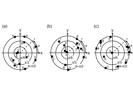
FIG. 3.: Distributions of principal-axis directions. (a), (b), (c). Data points represent the $\hat{h}_{1}$, $\hat{h}_{2}$, and $\hat{h}_{3}$ principal-axis directions, respectively, with circles for sample Cu#1 and squares for Cu#2. The numbers identify the energy levels (see Table I), in order of increasing excitation energy. $\theta$ and $\phi$ are spherical polar coordinates, with $\theta$ measured relative to $\hat{z}$, the direction perpendicular to the plane of the silicon nitride membrane. The radii of the circles of constant $\theta$ are scaled so that the areas inside the circles are proportional to the solid angle of the sphere with polar angle less than $\theta$.

of solid angle on the hemisphere are mapped to equal areas in Fig. 3. The principal axes for different quantum states clearly do vary widely, and there does not appear to be any clustering in particular directions.

In summary, we have made the first measurements of the angular dependence of the $g$-factors for spin Zeeman splitting for individual quantum states in quantum dots. The results verify the predictions that spin-orbit coupling can cause the spin properties of quantum states to depend sensitively on the direction of an applied magnetic field. When we compare the $g$-factors between different quantum states in the same nanoparticle, there are large variations both in angular dependence as well as magnitude, supporting the picture that the strong anisotropies arise from the intrinsic random variations of quantum-mechanical wavefunctions.

We thank Edgar Bonet, Mandar Deshmukh, and Eric Smith for help with the experimental setup, and Xavier Waintal, Shaffique Adam, and Piet Brouwer for discussions. This work was supported by the NSF, through DMR-0071631 and the use of the National Nanofabrication Users Network. Support was also provided by the Packard Foundation, ARO (DAAD19-01-1-0541), and a DoEd GAANN fellowship.

REFERENCES

- [1] S. A. Wolf et al., Science 294, 1488 (2001).
- [2] J. S. Moodera, J. Nassar, and G. Mathon, Ann. Rev. Mat. Sci. 29, 381 (1999).
- [3] H. Ohno et al., Appl. Phys. Lett. 69, 363 (1996).
- [4] D. Loss and D. P. DiVincenzo, Phys. Rev. A 57, 120 (1998).
- [5] C. P. Slichter, Principles of magnetic resonance (Springer-Verlag, New York, 1990).
- [6] J. E. Harriman, Theoretical foundations of electron spin resonance (Academic Press, New York, 1978).
- [7] P. W. Brouwer, X. Waintal, and B. I. Halperin, Phys. Rev. Lett. 85, 369 (2000).
- [8] K. A. Matveev, L. I. Glazman, and A. I. Larkin, Phys. Rev. Lett. 85, 2789 (2000).
- [9] K. S. Ralls, R. A. Buhrman, and R. C. Tiberio, Appl. Phys. Lett. 55, 2459 (1989).
- [10] J. R. Petta and D. C. Ralph, Phys. Rev. Lett. 87, 266801 (2001).
- [11] D. V. Averin and K. K. Likharev, Mesoscopic phenomena in solids (Elsevier, Amsterdam, 1999).
- [12] D. C. Ralph, C. T. Black, and M. Tinkham, Phys. Rev. Lett. 74, 3241 (1995). As described in this paper, the capacitance ratio can be determined by comparing the voltages at which a resonance peak is observed at positive and negative bias, or from the voltage shift that occurs when superconducting electrodes are driven normal.
- [13] D. G. Salinas, S. Guéron, D. C. Ralph, C. T. Black, and M. Tinkham, Phys. Rev. B. 60, 6137 (1999).
- [14] D. Davidović and M. Tinkham, Phys. Rev. Lett. 83, 1644 (1999).
- [15] American Magnetics, Inc. Oak Ridge, TN, 37831.
- [16] R. H. Hardin, N. J. A. Sloane, and W. D. Smith, http://www.research.att.com/njas/icosahedral.codes/index.html