Stripes and holes in a two-dimensional model of spinless fermions and hardcore bosons

Abstract

We consider a Hubbard-like model of strongly-interacting spinless fermions and hardcore bosons on a square lattice, such that nearest neighbor occupation is forbidden. Stripes (lines of holes across the lattice forming antiphase walls between ordered domains) are a favorable way to dope this system below half-filling. The problem of a single stripe can be mapped to a spin-1/2 chain, which allows understanding of its elementary excitations and calculation of the stripe’s effective mass for transverse vibrations. Using Lanczos exact diagonalization, we investigate the excitation gap and dispersion of a hole on a stripe, and the interaction of two holes. We also study the interaction of two, three, and four stripes, finding that they repel, and the interaction energy decays with stripe separation as if they are hardcore particles moving in one (transverse) direction. To determine the stability of an array of stripes against phase separation into particle-rich phase and hole-rich liquid, we evaluate the liquid’s equation of state, finding the stripe-array is not stable for bosons but is possibly stable for fermions.

I introduction

Stripes have been an area of active study in the high-temperature superconductivity research. They are modulations of charge and spin densities, and can be static or dynamic. In 1995, Tranquada and coworkersExp observed the coexistence of superconducting and stripe domain order for the material La_1.6-xNd_0,4Sr_xCuO₄ at around doping $x=0.125$. The stripes are one-dimensional objects on a two-dimensional plane, and they have been called “self-organized one dimensionality.”ZaanenScience Search for stripes in the Hubbard and $t-J$ models has been intense and is still going strong (see Ref. EmKi, for a review of some experimental results and theoretical considerations).

¿From the theory side, there are basically two roads. One approach is using microscopic models such as the Hubbard and $t-J$ models to study numerically stripe formation and phase separation. DMRG appears to be the best tool in such studies and has been applied to the $t-J$ model in Refs. dmrg1, ; dmrg2, . Another approach to stripes is to use effective field theories, treating stripes as macroscopic objects (macrosopic in the sense of many-particle collective motion). For example in Ref. Zaanenstrings, , Zaanen considered stripes as “a gas of elastic quantum strings in $2+1$ dimensions.” The microscopic, numerical approach can be used to understand the mechanism for stripe formation and to derive macroscopic parameters such as stripe-stripe interaction energy and stripe stiffness, but it is limited by computational power. The macroscopic approach on the other hand takes these macroscopic parameters as an input and can obtain results relevant to experiments, but it can explain less about mechanism. We will follow the microscopic route which enables us to obtain macroscopic parameters from diagonalization data.

I.1 The model

In this paper, we study stripes in a strongly-interacting model of spinless fermions and hardcore bosons on the square latttice. The Hamiltonian is

$$H=-t\sum_{\langle i,j\rangle}\left(c^{\dagger}_{i}c_{j}+c^{\dagger}_{j}c_{i}\right)+V\sum_{\langle i,j\rangle}\hat{n}_{i}\hat{n}_{j},$$ (1)

with periodic boundary conditions. We study both the spinless fermion and the hardcore boson versions of the model. $c^{\dagger}_{i}$ and $c_{i}$ are the spinless fermion or hardcore boson creation and annihilation operators at site $i$, $\hat{n}_{i}=c^{\dagger}_{i}c_{i}$ the number operator, $t$ the nearest-neighbor hopping amplitude, and $V$ the nearest-neighbor interaction. At the each site there can be at the most one particle. Furthermore, we study the strong-correlation limit of the model and take $V=+\infty$, i.e., infinite nearest-neighbor repulsion.

The spinless fermion and hardcore boson model with infinite nearest-neighbor repulsion involves a significant reduction of the Hilbert space as compared to the Hubbard model. The Hubbard model on the $4\times 4$ lattice at half-filling, with 8 spin-up and 8 spin-down electrons has $1,310,242$ states in the largest matrix block, after reduction by particle conservation, translation, and the symmetries of the square.Lin In our model with infinite $V$, after using particle conservation and translation symmetry (but not point group symmetry), the largest matrix for the $7\times 7$ system has $1,906,532$ states (for 11 particles). We can therefore compute for all fillings the $7\times 7$ system whereas for the Hubbard model $4\times 4$ is basically the limit. This also means that at certain limits we can obtain results that are difficult to obtain in the Hubbard model, for example, we can exactly diagonalize a system of two length-8 stripes on the $8\times 28$ lattice.

This is one of the two papers that we are publishing to systematically study the phase diagram of the spinless fermion and hardcore boson model on the square lattice with infinite nearest-neighbor repulsion. In the other paper, dilutepaper we study the dilute limit of this model Eq. (1), focusing on the problem of a few particles, and that limit is dominated by two-body interactions. In the present paper, we study the near-half-filled limit of our model, where stripes are natural objects.

With infinite nearest-neighbor repulsion, the maximum filling fraction (particle per site) for our model is 1/2, for both spinless fermions and hardcore bosons. At exactly half-filling, the particles form a checkerboard configuration that cannot move. Adding a single hole to it cannot produce motion either because the hole is confined by neighboring particles. A natural way to add holes to this system is to align them in a row going across the system, as indicated in Fig. 1. We call this row of holes a stripe and it is the subject of study in this paper.

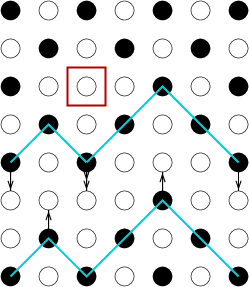
Figure 1: An isolated hole (shown in the box) in a half-filled region cannot move. A row of holes (a stripe) can slide along in the vertical direction, with the arrows showing the possible moves.

For many systems with certain aspect ratios (e.g., the $6\times 7$ lattice depicted in Fig. 1), the stripe state is the one with the smallest number of holes and nonzero energy. Here we have an interesting kind of physics of extended, fluctuating, quantum mechanical objects, that are results of collective motions of many particles.

Spinless models related to the present one have been invoked occasionally in the literature Ko67 but usually in the context of a specific question about spinfull models: it was recognized that a spinless model would capture the same physics with fewer complications. The only systematic work on phase diagram of spinless fermions is by Uhrig. uhrig However, the method is expansion around infinite dimensionality; this will have special difficulty with arrays of domain walls, since wall fluctuations and the attendant kinetic energy are strongly suppressed in high dimensions.

The Falicov-Kimball model is an alternate way to simplify the Hubbard model, which is also commonly presented in a spinless form, free93 and develops stripe-like incommensurate patterns. free02 However, this model includes a second immobile (classical) species of electron, so its stripes cannot have quantum fluctuations. Ba-KBiO3

No known electron system realizes our model, even approximately. A “half-metallic” ferromagnet halfmetal ; Cu71 – meaning that for one spin state, the conduction band is all filled or all empty – realizes a spinless model for the other spin state. However in the best-known half-metals, the manganites, Pa98 the formation of inhomogeneities is dominated by lattice distortions and orbital degeneracies (not to mention static pinning disorder), so that quantum-fluctuating defects find no role in current theories of manganites. (The same may be true for the Verwey transition in magnetite, seo which was modeled previously with spinless electrons Cu71 .) Conceivably the spinless model could be realized in an array of semiconductor quantum dots in a magnetic field. manousakis

The most plausible realization of the boson version of our model would be an adsorbed gas of ⁴He on a substrate with square symmetry. (The same model – but on a triangular lattice – has been introduced independently to model ⁴He on nanotube green00 ; green02 ). The fermion case could similarly be realized, in principle, by spin-polarized ³He, however it would be difficult to achieve a degree of polarization sufficient to neglect the minority spin state.

This paper appears to be the first using exact diagonalization (as opposed to DMRG) to investigate the properties of interacting stripes with a microscopic Hamiltonian. FN-EDstripe

I.2 Stripes in spinfull models

In real fermion systems, stripes (antiphase domain walls containing holes) have been a prominent object of experimental study in the high-$T_{c}$ cuprates. Exp ; EmKi ; Zaanenrev ; Whiterev ; Baskaran Stripe-based mechanisms have been proposed for high-temperature superconductivity, EmKi-SC ; EmKi but the prevalent current opinion is that stripes compete with superconductivity. Zaanenrev ; Whiterev ; Baskaran

Nevertheless, stripes are obviously clues to how the charge and spin degrees of freedom interact with each other, which is important in a majority of the high-$T_{c}$ theories. Stripes are modeled theoretically and numerically using the same Hubbard model (or its variations) which were already accepted as models of homogeneous phases. It is still unsettled whether stripes are stabilized in this model, which omits long-range and even nearest-neighbor Coulomb repulsion. The most explicit calculations are by Density-Matrix Renormalization Group (DMRG), adapted to two-dimensional systems formed into strips. dmrg1 ; dmrg2 The results favor stripes with 1/2 holes per unit length, as found in experiments; however, those simulations are strongly influenced by the (necessary) open boundary conditions on two sides.

What relation can our spinless model have to these spinfull models? Firstly, at the intermediate scales appropriate to a stripe array, the spinfull and spinless systems are modeled in very similar ways: stripes are mutually repelling, quantum-fluctuating strings. This level is appropriate to studies of the anisotropic transport expected in a (non-superconducting) stripe array, as well as the stripe interactions, as has been emphasized by Zaanen. zaanen ; Eskes ; Zaanenstrings In the spinfull models, only a little has been done to explicitly relate the macroscopic parameters to the underlying microscopic model. smith In our model – and unlike any spinfull model – exact diagonalization can address phenomena such as the effective mass and interactions of carriers on a stripe, long-wavelength stripe fluctuations, stripe-stripe repulsion, or the transfer of carriers from one stripe to the next. Thus, not only analytically but numerically, one can go quite far in extracting such parameters for our model.

Secondly, if spinfull stripes are stabilized at all (in the absence of long-range repulsion), it is by kinetic energy in the same fashion that our stripes are stabilized. In either case, a fermion belonging to one domain hops transverse to the stripe, and (since the stripe is also an antiphase domain wall) still finds itself correctly placed in the order of the new domain. In our model, that order is the “checkerboard” pattern, which is enforced by the nearest-neighbor repulsion $V$. From this viewpoint, $V$ is analogous to the antiferromagnetic coupling $J$ in the $t$-$J$ model. (Our $V\to\infty$ limit then corresponds to the case $J\gg t$, which is the unphysical regime of the $t$-$J$ model.)

An even more precise correspondence would be to stripes in the $t$-$J_{z}$ model: Tch ; CherNeto00 in that system (as in ours) the undoped, ordered state breaks a discrete (Ising-type) symmetry, and hence is practically inert, supporting no gapless Goldstone (spinwave) excitations: only the stripe itself has low-energy excitations. If the ordered state had a continuous symmetry, as in the Hubbard or $t$-$J$ models, spin-wave modes can mediate a $1/d^{2}$ attraction Pryadko98 between stripes (where $d$ is the stripe separation). If short-distance kinetic energy were to favor a stripe array, the long-range force mediated by continuous spins implies phase separation in the limit of very small doping. FN-Casimir

Our stripes with an occupation of 0.5 hole per unit length are insulating and correspond to insulating stripes of 1 hole per unit length in the $t$-$J$ model (the factor of two reflects the density of the ordered background state), as implied in the original ideas Pre93 ; Pre94 ; Zaanenrev about stripe stabilization from a strong-coupling viewpoint.

I.3 Paper organization

This paper is organized as follows. First (in Sec. II) we describe briefly our exact diagonalization code for studying the near-half-filled limit of our model. We use translation symmetry to block diagonalize the Hamiltonian matrix. A graph viewpoint motivates a method of building the basis states from a starting configuration and explains the relation between boson and fermion energy spectra.

Next (Sec. III) we study the problem of a single stripe. Here particles can only move in one direction, effectively reducing the 2D problem to a 1D one. This one-stripe problem maps exactly to a spin-1/2 chain, which is exactly solvable using Bethe ansatz. Using the single-stripe energy dispersion relation along the direction perpendicular to the stripe, we obtain stripe effective mass for motion in that direction.

In the next two sections, we study the problem of one or two holes on a stripe. (For the one-hole case, the bosons and fermions have the same energy spectrum.) We determine the dispersion relationship (energy gap and effective mass) for one hole moving on a stripe, and study the binding of two holes. It is informative to study the finite-size dependence of the energy on the lattice dimensions in both directions: in particular, it decays exponentially as a function of the lattice size perpendicular to the stripe, which we explain quantitatively in terms of the stripe tunneling through a barrier between two potential wells.

One of the motivations for studying our model is our interest in a simple model of interacting stripes. In Sec. VI we have exactly diagonalized systems with two, three, and four stripes, and find that the stripes repel. The interaction energies scale as the inverse square of the stripe spacing, which (like the above-mentioned tunneling) follows from the one-dimensional nature of the stripe’s transverse motion in our systems.

Finally (Sec. VII) we discuss the stability of an array of stripes by fitting the diagonalization results in the intermediate filling limit and using a Maxwell construction. Our interest is whether at the intermediate-filling limit we have the stripe-array case or a phase-separated case with hole-rich regions and particle rich-regions. The conclusion is, interestingly, that the boson stripe-array is not stable and the fermion stripe-array is very close to the stability limit and is possibly stable.

Our earlier publication, Ref. HenleyZhang, , contains some of the results of this paper in a condensed form, with a focus on the stability of the stripe-array. The present paper contains more systematic and more updated results and a substantial number of important new results on, for example, boson and fermion statistics, stripe effective mass and stripe-stripe interaction.

II Basis States and Diagonalization Program

In this section, we describe our exact diagonalization code. We begin by describing the conventions for labeling basis states, which are crucial to keep track of sign factors in the fermion case. Then we introduce a geometrical way to view the basis states as nodes on a graph, and apply this to classify the conditions under which the boson and fermion problems have the same.

Figure 2: Square lattices with periodic boundaries: $(4,0)\times(0,5)$ on the left and $(4,1)\times(1,5)$ on the right. Site numbers are shown, following the numbering convention, upward and rightward.

II.1 Basis states

Each basis state with $M$ particles corresponds 1-to-1 to a configuration, which is array of the $M$ occupied site numbers $(i_{1},i_{2},...,i_{M})$. Any configuration with two nearest neighbors occupied is excluded because of the infinite $V$ in the Hamiltonian Eq. (1). Periodic boundary conditions are specified by two lattice vectors ${\bf R}_{1}$ and ${\bf R}_{2}$ (which will be called boundary vectors in the following), such that for any lattice vector ${\bf r}$ we have ${\bf r}+n_{1}{\bf R}_{1}+n_{2}{\bf R}_{2}\equiv{\bf r}$, where $n_{1}$ and $n_{2}$ are two integers.

The configuration by itself is insufficient to define the basis ket, since we need to specify its sign or phase factor. To fix the fermion sign, we must establish an arbitrary ordering of sites and always configurations in this order. Then we denote the basis state $|n\rangle=c^{\dagger}_{i_{1}}c^{\dagger}_{i_{2}}...c^{\dagger}_{i_{M}}|0\rangle$,

The site ordering convention used in this paper is to start with site 0 at the lower left corner and move upward along a lattice column until we encounter the cell boundaries defined by the boundary vectors ${\bf R}_{1}$ and ${\bf R}_{2}$, then shift rightward and repeating in the next column, progressing until all sites have been numbered. Fig. 2 shows two example systems: $(4,0)\times(0,5)$ and $(4,1)\times(1,5)$.

In this basis the Hamiltonian Eq. (1) acts as

$$H|n\rangle=(-t)\sum_{m\in{\cal M}}s(n,m)|m\rangle,$$ (2)

where ${\cal M}$ denotes the set of states created by hopping one particle in $|n\rangle$ to an allowed nearest-neighbor site. For bosons $s(n,m)=1$ always and for fermions $s(n,m)=\pm 1$. And the matrix element is $\langle m|H|n\rangle=-s(n,m)t$ if $m\in{\cal M}$ and 0, otherwise.

We use lattice translation symmetry to block diagonalize the Hamiltonian matrix $\langle m|H|n\rangle$. The eigenstates that we use are the Bloch statesLeung

$$|n,{\bf k}\rangle=\frac{1}{N_{n{\bf k}}}\sum_{l=0}^{N-1}e^{-i{\bf k}\cdot{\bf R}_{l}}T_{l}|n\rangle.$$ (3)

In this expression ${\bf k}$ is a reciprocal lattice vector (one of $N$, where $N$ is the number of sites), ${\bf R}_{l}$ is a lattice vector (the order of $l$ in the sum is not important), $T_{l}$ is translation by ${\bf R}_{l}$, and $N_{n{\bf k}}$ is a normalization factor. The original basis states $|n\rangle$ are divided by translation into classes and any two states in the same class give the same Bloch state with an overall phase factor. A representative is chosen from each class and is used consistently to build the Bloch states. For a state $|n\rangle$ we denote its representative $|\bar{n}\rangle$, and the Hamiltonian matrix is block diagonal in the sense that $\langle\bar{m},{\bf k}^{\prime}|H|\bar{n},{\bf k}\rangle=0$ when ${\bf k}^{\prime}\neq{\bf k}$. The matrix $\langle\bar{m},{\bf k}|H|\bar{n},{\bf k}\rangle$ is diagonalized for each ${\bf k}$ vector using the well-known Lanczos method.

II.2 State graph

It is helpful conceptually to represent specific cases of our Hamiltonian by the state graph, in an abstract (or high-dimensional) space, such that each node corresponds to a basis state, and two nodes are joined by an edge of the graph if and only if the two states differ by one particle hop. (As used in Sec. III.1, our many-body Hamiltonian is almost equivalent to a single particle hopping on the state graph.) The best-known precedent of this approach s Trugman’s study of one-hole and two-hole hopping in the $t$–$J_{z}$ model Trugman .

Two states are connected if one state can be changed to another by a succession of hops. For states near half filling, our $V=\infty$ constraint forbids many hop moves, so the graph is sparse and can possess interesting topological properties relevant to our spectrum.

II.2.1 Droplets and accessibility of states

We remarked (Fig. 1) that an isolated hole is unable to hop; larger finite “droplets” of holes are still immobile, though they may gain kinetic energy from internal fluctuations. Specifically, Mila if one draws a rectangle with edges at $45^{\circ}$ to the lattice around the droplet, so as to enclose every site which deviates from the checkerboard order, then (with the $V=\infty$ constraint) sites outside this rectangle can never be affected by fluctuations of the droplet.

Due to the droplets, the state graph (representing all states with $M$ particles) may be broken up into many disconnected components, states which cannot access each other by allowed hops. This happens if both boundary vectors are even vectors, so that the system cell would support half filling with a perfect checkerboard order. For slightly less than half filling, the typical basis state consists of scattered immobile droplets of the kind just described. Each component corresponds to a different way to assign the holes to droplets, or merely a shifted way of placing the same droplets. Each sort of droplet has its characteristic energy levels FN-smalldroplets and the system energies are the sum, just like a system of noninteracting atoms, each having its independent excited levels.

When the state graph is disconnected, the Hilbert space is correspondingly blocked into components which are not connected by matrix elements. This is beyond the blocking according to translational symmetry, which remains true.

II.2.2 Building basis set from a starting configuration

In systems with even-even boundary conditions, we are not mainly interested in the configurations with droplets, but in those with two stripes. FN-stripevsdroplet Since these are disconnected from the rest of the Hilbert space, it speeds up the the diagonalization by a large factor if it is limited to the stripe-configuration subblock of the Hamiltonian matrix. The only way to separate out this subblock is to generate basis states iteratively from a starting configuration which has two stripes.

What of the case of even-odd or (equivalently) odd-odd boundary conditions? These force one stripe (possibly with additional holes, or possibly more stripes). In every such case (excluding $L\times L$ with odd $L$), the stripe can fluctuate and absorb any droplets, so we believe the Hilbert space is fully connected, and the diagonalization is not speeded up. Nevertheless, for every case near half-filling, we enumerated the basis from a starting configuration, as (we believe) this is the fastest way to do so. Systematically enumerating all possible fillings by brute force would take more time than the diagonalization itself, since almost every brute-force trial configuration gets ruled out by the $V=\infty$ constraint.

However, at low fillings (which we study in Ref. dilutepaper, ) the brute-force enumeration is used. In that case, if we generated from a starting configuration, there would be too many alternate routes to reach a given state. Hence much time would be wasted in searches to check whether each newly reached state was already on the basis state list.

Below we outline the algorithm for building the basis states and the Hamiltonian matrix.

Figure 3: Building basis states from a given state $n$. Applying all allowed hoppings to $n$ (the level 0 state) gives the states $n_{1}$, $n_{2}$, $n_{3}$, … Applying hoppings to $n_{1}$ (a level 1 state) gives level 2 states $n_{11}$, $n_{12}$, $n_{13}$, … The basis state list is then $n$, $n_{1}$, $n_{2}$, $n_{3}$, …, $n_{11}$, $n_{12}$, $n_{13}$, …, $n_{21}$, $n_{22}$, …, $n_{111}$, $n_{112}$, … Note that when applying hoppings to a state, only add states not already on the list. We call this graph of states connected by hopping the state graph.

To build basis states without using translation symmetry from a starting state $n$, we follow the following steps.

1. Apply hopping to $n$ and obtain states $n_{1}$, $n_{2}$, $n_{3}$,… See Fig 3. Form the basis state list $n$, $n_{1}$, $n_{2}$, $n_{3}$,… that are numbered 0, 1, 2, 3,… And record the Hamiltonian matrix elements $H_{0,1}$, $H_{0,2}$, $H_{0,3}$,…

2. Apply hoppings to the next state on the basis state list that has not been applied hopping to. Here from $n_{1}$ we get $n_{11}$, $n_{12}$, $n_{13}$… Add these to the basis state list to form $n$, $n_{1}$, $n_{2}$, $n_{3}$, …, $n_{11}$, $n_{12}$, $n_{13}$, … (Note we should not add states that are already on the list. For example, applying hoppings to $n_{1}$ will certainly give $n$ back again. Do not include this state in level 2 states. When computing Hermitian matrix elements we only need $H_{p,q}$ for $p<q$.) If $n_{11}$ is the $m$-th element on the list, record the matrix elements $H_{1,m}$, $H_{1,m+1}$, $H_{1,m+2}$,…

3. Repeat the previous step until all the states on the list have been applied hopping to and no new states are created.

We finish with a basis state list $n$, $n_{1}$, $n_{2}$, $n_{3}$, …, $n_{11}$, $n_{12}$, $n_{13}$, …, $n_{21}$, $n_{22}$, …, $n_{111}$, $n_{112}$, … And we have stored the Hamiltonian matrix elements.

When building basis states with translation symmetry, as in Eq. (3), the procedure is like the above, except we apply hopping to representative states of each class of translation related states and also store the representatives of the resulting states.

II.3 Boson and fermion statistics

In this paper we study both the boson and the fermion versions of our model Eq. (1), and one question that we often ask is when bosons and fermions have the same spectrum. In this section, we introduce a graph-based way to study the relationship between the boson and fermion spectra.

Using Eq. (2), we know that if $\beta$ is a state that can be obtained from the state $\alpha$ by one nearest-neighbor hop, then we have

$$\langle\beta|H|\alpha\rangle_{f}=s(\beta,\alpha)\langle\beta|H|\alpha\rangle_{b},$$ (4)

where the subscripts $f$ and $b$ denote the fermion and boson matrix elements respectively and we have used the fact that $s(\beta,\alpha)=1$ for bosons. If we can write

$$s(\beta,\alpha)=\sigma(\beta)\sigma(\alpha),$$ (5)

i.e., $s(\beta,\alpha)$ as a product of a function $\sigma$ that depends on one state only, then Eq. (4) can be written as a matrix equation,

$${\bf H}_{f}={\bf\Sigma}{\bf H}_{b}{\bf\Sigma},$$ (6)

where $\Sigma_{\alpha,\beta}=\delta_{\alpha,\beta}\sigma(\alpha)$. Because ${\bf\Sigma}={\bf\Sigma}^{-1}$, it is a similarity transformation, and then the eigenvalues of ${\bf H}_{f}$ are identical to that of ${\bf H}_{b}$. Indeed, this is a much stronger condition than having identical eigenenergy spectra: the eigenstates are also identical (modulo a sign), so e.g. an operator which depends on the basis state has the same expectation in the boson and fermion cases. On the other hand, if the function $\sigma$ cannot be defined, the boson and fermion Hamiltonians are not equivalent.

We can relate Eq. (5) to the loops which occur in virtually every state graph with the help of Fig. 4. Here $s(\beta,\alpha)$ is defined on the arrow pointing from $\alpha$ to $\beta$, whereas the function $\sigma(\alpha)$ is defined on the node $\alpha$ of the graph.

Figure 4: Obtaining $\sigma(\alpha)$, that is defined for each state, from a reference state 0 and the step wise hopping sign function $s(\beta,\alpha)$, that is defined on the arrow pointing from $\alpha$ to $\beta$. Define $\sigma(\beta)=s(\beta,\alpha)\sigma(\alpha)$. If the function $\sigma(\beta)$ is well-defined, i.e., all paths leading from 0 to $\beta$ give the same sign, then the boson and fermion spectra are identical.

Fig. 4 suggests a natural way to construct $\sigma(\alpha)$. First we choose a reference point. This should not matter and the one we choose is the starting state of the exact diagonalization program, say $0$. We set $\sigma(0)=1$. Then if one hop takes $\alpha$ to $\beta$, define $\sigma(\beta)=s(\beta,\alpha)\sigma(\alpha)$. This is certainly correct if Eq. (5) is true; but if the state graph has a loop, two different paths lead to the same state $\beta$ from 0, and $\sigma(\beta)$ can be well defined only if they produce the same sign. The answer is different for different state graphs (or disconnected subgraphs of the state graph), so it depends on the system dimensions and filling.

We can check numerically whether the function $\sigma(\alpha)$ is well defined at the same time as we are building the basis set by applying hopping, i.e. constructing the state graph in the form of a tree (Fig. 3). We store a sign for each state, starting with $\sigma(n)=1$ for state $n$ in Fig. 3. As we expand the tree, we compute the sign for the next level of states. Whenever we come to a state that is already on the list, we test whether the sign we produce following the current path equals that already stored for that state. Depending whether the sign always agrees or sometimes disagrees, we know the fermion and boson problems are or are not equivalent. This method is the basis for statements later in the paper on boson and fermion spectra (Sec. III.1 and Sec. VI.1, and briefly in Secs. IV and V); it is not necessary to compute all the eigenvalues.

The boson-fermion equivalence condition can be re-stated in a way that is independent of the site ordering convention at the start of Sec. II. Say each particle is originally numbered $1,\ldots,M$ and retains its number when it hops. Then $\sigma(\alpha,\beta)$ is simply the sign of the permutation which changes the string of particles (when they are listed according to the site order). The function $\sigma(\alpha)$ is well-defined if and only if the product of $\sigma(\alpha,\beta)$ around any closed loop of the state graph is unity; in other words, if and only if any sequence of hops that restores the original configuration induces an even permutation of the particles. When just two particles can be exchanged (an odd permutation), as is obviously possible at low fillings, the fermion and boson spectra are obviously different.

III A Single Stripe

It was first observed by Mila, in a model very similar to ours, that the creation of stripes is more favorable than of isolated holes, as a way to dope the system below half filling. Mila ; HenleyZhang We shall finally address more rigorously the phase stability of the stripe (Sec. VII), but in this section we will study the eigenstates of a single stripe in the system. In Fig. 5 we show a $L_{x}=4$ and $L_{y}=7$ system with 12 particles. A stripe of length four is formed along the $x$ direction. The only four possible nearest-neighbor hops of the leftmost state are indicated with arrows and the resulting four states are shown on the right. Note that with a single stripe, the particles can only hop in the $y$ direction. It is not possible for them to move in any fashion in the $x$ direction.

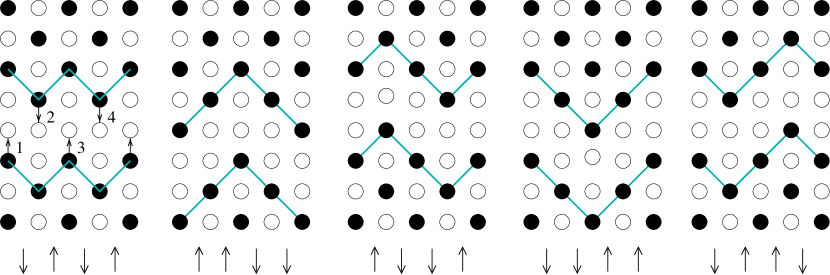
Figure 5: A single stripe in the $4\times 7$ system. For the leftmost state, the four possible hops are labeled and the resulting configurations are shown on the right. The corresponding spin chain configurations are shown below (see Sec. III.2).

We also consider tilted boundaries $(L_{x},b)\times(0,L_{y})$, which force a tilt of $b$ steps to the stripe because the site $(0,y)$ is identified with $(L_{x},y+b)$. In Fig. 6, the $(5,1)\times(0,7)$ and $(6,2)\times(0,7)$ systems are shown. Note because each stripe step is at 45 degree angle, an even (odd) horizontal length of the stripe $L_{x}$ must produce an even (odd) number of total vertical steps $b$. Thus $L_{x}+b$ is always even. For a general $(L_{x},b)\times(0,L_{y})$ system with $L_{y}$ odd, the single-stripe states have $M=L_{x}(L_{y}-1)/2$ particles. Note also that for the tilted stripes, vertical hopping is again the only allowed motion of the particles.

Diagonal stripes are observed in La₂NiO₄,Exp and they are an interesting topic in the $t-J$ model.smith However, in our model with $V=\infty$, no hopping is possible away from a $45^{\circ}$ edge of any domain. Thus a diagonal stripe has no kinetic energy (unless there are additional holes, as discussed in Sec. IV.4) and is disfavored.

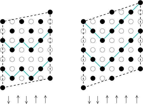
Figure 6: A single stripe in the $(5,1)\times(0,7)$ and the $(6,2)\times(0,7)$ systems. The boundary conditions force a tilt of the stripe. The corresponding spin-chains have total $S_{z}$ equal to $1/2$ and $1$ respectively (see Sec III.2).

III.1 Boson and fermion statistics for one stripe

We find from diagonalization that for one-stripe systems with rectangular boundaries, the boson and fermion spectra are identical and are symmetric about zero. For a stripe in systems with tilted boundaries, there are complications. For the $(2m+1,1)\times(0,2l+1)$ system, with $m$ and $l$ integers, the spectrum is not symmetric about zero. In this case, with $l$ odd, the fermion spectrum is still identical to the boson spectrum, but for $l$ even, the fermion energies are the boson ones with a minus sign (and because the spectrum is no longer symmetric about zero, the fermion energies are not the same as the boson energies). For the $(2m,2)\times(0,2l+1)$ system, the boson and fermion spectra are identical and symmetric about zero.

All these numerical findings can be explained in terms of the state graph, extending Sec. II.3. We must characterize the permutations induced by a sequence of particle hops which return to the same basis configuration. This is quite easy in the single stripe state, since (as already commented on Fig. 5 and Fig. 6), particles move in the $y$ direction only. Our discussion includes all $(L_{x},b)\times(0,L_{y})$ systems (which are tilted boundaries if $b\neq 0$). In these cases, particles are confined to the same column, and the net permutation is a product of permutations in each column.

Consider the total particle permutation induced when the system returns to the starting state by a loop on the state graph. FN-signrule If in this process the stripe as a whole makes no net movement across the $y$ boundaries, then in each column the particles undo their hops and the net permutation is the identity. Thus, the only nontrivial loops are those in which the stripe crosses the $y$ boundary. Indeed, since each hop moves the stripe locally by $\Delta y=\pm 2$, the stripe must cross it must cross the boundary twice. The particles in each column have returned to the original positions with a cyclic permutation in each column, which has the sign

$$\sigma_{\rm col}\equiv(-1)^{(L_{y}+1)/2}$$ (7)

Therefore the sign of the system’s permutation is ${\sigma_{\rm col}}^{L_{x}}$ which (since $L_{x}+b$ is even) reduces to $(-1)^{b(L_{y}+1)/2}$: the fermion and boson spectra differ if and only if this phase is $-1$, i.e. only when $b$ is odd and $L_{y}\equiv 1\pmod{4}$.

The $\pm E$ symmetry of the single-stripe spectrum also falls out from visualizing the Hamiltonian as a single particle hopping on the state graph (with amplitude $-t=-1$ for every graph edge), and recalling the spectrum depends only on the attributes of closed loops. We can always change our convention for the phase factors of the basis states, which is equivalent to a “gauge transformation” on the nodes of the state graph. Whenever a state graph is bipartite, meaning every closed loop on it has an even number of edges, it is well-defined to divide the basis states into “even” and “odd” classes. If we change the phase factor by $-1$ for every “odd” basis state, every edge (every $s(n,m)$ factor) picks up a factor $-1$. By gauge equivalence, the new Hamiltonian matrix has the same spectrum. Yet on the other hand, it is manifestly the same as the old matrix with $t\to-t$, so it has the sign-reversed spectrum; this proves the $\pm E$ symmetry. Now, the nontrivial loops in the state-graph are those that pass the stripe twice across the $y$ boundary; this motion requires $L_{x}L_{y}\equiv N$ hops. Thus, the state-graph is bipartite and the spectrum has $\pm E$ symmetry, if and only if $N$ is even.

If $N$ is odd, the gauge-invariant effect of reversing $t\to-t$ is to change the net product of $s(n,m)$ around every nontrivial loop by a factor $-1$. But we showed that switching Fermi and Bose statistics creates the same sign: hence the fermion spectrum is the inverse of the boson spectrum, as observed.

III.2 Mapping to spin chain

In Figs. 5 and 6, we have indicated a natural map from any configuration $y(x)$ of the stripe to a state of a spin chain of length $L_{x}$. (Recall that “configuration” was defined in Sec. II.1 as a pattern of occupied sites; the map from the quantum states of the stripe is more subtle on account of phase factors, which are confronted later in this subsection.) Here it is obvious the spin length is one-half, for each stripe step, $y(x+1)-y(x)$, can take only two values.FN-Tch The up step of the stripe is mapped to an up spin and the down step to a down spin. For example, the leftmost configuration in Fig. 5 maps to a spin state $|\downarrow\uparrow\downarrow\uparrow\rangle$. This mapping was first noted by Mila Mila , who used it (as we do here) to evaluate the exact ground state energy of a stripe.

Note that when the periodic boundary conditions are rectangular, the stripe satisfies $y(L_{x})=y(0)$. In the corresponding states of the spin chain, the total $z$ spin component is zero. For tilted boundaries, the map to the spin-chain works exactly as before, the only difference being that the resulting spin configurations have $\sum_{i}{S_{i}^{z}}=b/2$.

The stripe-to-spin-chain map is not one-to-one, for translation in the $y$ direction of a single-stripe state gives the same spin-chain state (with a possible fermion sign). A rather analogous situation (but one dimension higher) appears in the two-dimensional quantum dimer model (QDM). rokhsar ; henleydimer In the QDM, every dimer configuration corresponded with a surface $z(x,y)$, uniquely except for an arbitrary shift of $z$, just as our spin (or 1D fermion) chain corresponds to a stripe $y(x)$ here. There were two kinds of low energy excitations of the QDM: ripplon modes of the “surface”, and transverse motion (or tunneling) of the “surface” through a periodic boundary condition. These correspond, respectively, to our ripplon modes labeled by $k_{x}$ (see Sec. III.3.1 and also Sec. IV) and to our $y$-translation modes labeled by $k_{y}$ (see Eq. (29)). The analogy is imperfect in that, in the QDM, the dimer configuration is “real” and the surface is an abstract mapping of it, whereas here the spin chain is the abstract mapping and the stripe is “real.”

III.2.1 Spin Hamiltonian

To determine the Hamiltonian in spin language, consider that each allowed particle hop takes the stripe either from up-step/down-step to down-step/up-step or from down-step/up-step to up-step/down-step. They correspond to the nearest-neighbor spin flips $\uparrow\downarrow$ to $\downarrow\uparrow$ and $\downarrow\uparrow$ to $\uparrow\downarrow$ respectively.

Since the matrix element of $H$ is $-t$ between states differing by a hop, this must also be the matrix element of $H_{\rm spin}$ between states differing by a spin flip. Thus the equivalent spin Hamiltonian is

$$H_{\rm spin} = (-t)\sum_{i}\left(S_{i}^{+}S^{-}_{i+1}+S^{-}_{i}S^{+}_{i+1}\right)$$ (8)

$$= (-2t)\sum_{i}\left(S_{i}^{x}S^{x}_{i+1}+S^{y}_{i}S^{y}_{i+1}\right),$$

which is the so-called spin-1/2 XX chain and is well-studied and exactly solvable. Lieb

III.2.2 Mapping stripe states to spin states

Lifted to act on Hilbert space, the map should take the mathematical form

$${\cal S}|n\rangle=|n_{s}\rangle,$$ (9)

where $|n\rangle$ is a stripe state and $|n_{s}\rangle$ is a spin state.

Correspondingly, the equivalent spin Hamiltonian should satisfy

$${\cal S}H|n\rangle=H_{\rm spin}|{\cal S}n\rangle$$ (10)

where $H$ is the spinless fermion or hardcore boson Hamiltonian, Eq. (1), and $|n\rangle$ is any single-stripe state.

However, in the fermion case these equations are inconsistent with an arbitrary site-ordering scheme, for Eq. (9) did not take the sign factors into account. For many boundary conditions, there is no way to define a unique function, on account of the large loops in the state graph illustrated in Fig. 4. That is, particles can be hopped successively (corresponding to a walk on the state graph) such that $|n\rangle$ returns to the state $-|n\rangle$. This gauge-like phase is familiar from the spinor coherent states (where each spin direction is mapped to a spin-1/2 ket), in which case a $2\pi$ rotation induces a $-1$ phase shift. This is handled most transparently after a further mapping of the spin chain to a fermion chain (Sec. III.3, below). In that representation, the phase factor can be associated with the hopping of a one-dimensional fermion across the periodic boundary, and it will be implemented by adding an artificial flux that pierces the ring formed by the chain with periodic boundary conditions (Sec. III.4).

III.2.3 Special case: zero gauge phase

The many-to-one nature of the map (because $y\to y+2$ translation of the stripe produces the same spin state) is easier to handle. Let us choose a rectangular system, adopt the site-ordering conventions of Sec. II.1, and provisionally assume there is no gauge-like phase ambiguity. We ask that if $T_{R_{y}}$ translates a state in the $y$ direction by $R_{y}$, then ${\cal S}T_{R_{y}}|n\rangle={\cal S}|n\rangle$. One way to recover the notion of a unique map is to form Fourier states like Eq. (3), but only in the $y$ direction:

$$|n,k_{y}\rangle=\frac{1}{\sqrt{L_{y}}}\sum_{R_{y}}e^{-ik_{y}R_{y}}T_{R_{y}}|n\rangle.$$ (11)

The normalization factor here is always $1/\sqrt{L_{y}}$ because the $L_{y}$ translations in the sum cannot produce two identical states. From group theory we know $\langle m,k_{y}^{\prime}|H|n,k_{y}\rangle=0$ if $k_{y}\neq k_{y}^{\prime}$, so states with different $k_{y}$ belong to disconnected blocks. In each block with a given $k_{y}$, there is a one-to-one correspondence $|n,k_{y}\rangle\leftrightarrow{\cal S}|n\rangle$.

Using Eq. (2), because $H$ commutes with translation $T_{R_{y}}$, it is easy to show that

$$H|n,k_{y}\rangle=(-t)\sum_{m\in{\cal M}}s(n,m)|m,k_{y}\rangle.$$ (12)

For $q\in{\cal M}$, we then have

$$\langle p,k_{y}|H|n,k_{y}\rangle=-s(n,p)t.$$ (13)

But if we translate $p$ by $R_{y}$ so we have $T_{R_{y}}|p\rangle=\sigma|p^{\prime}\rangle$, where $\sigma$ is the fermion sign from translating the state $p$ by $R_{y}$, then the translation state $|p^{\prime},k_{y}\rangle=\sigma e^{ik_{y}R_{y}}|p,k_{y}\rangle$. Then we have,

$$\langle p^{\prime},k_{y}|H|n,k_{y}\rangle=-s(n,p)\sigma e^{-ik_{y}R_{y}}t.$$ (14)

Eqs. (14) and (13) tell us that choosing $p^{\prime}$ rather than $p$, the matrix element $\langle p^{\prime},k_{y}|H|n,k_{y}\rangle$ has an extra sign $\sigma$ and an extra phase factor $e^{-ik_{y}R_{y}}$. However, in the spin-chain language, we have, $\langle{\cal S}p|H_{\rm spin}|{\cal S}n\rangle=\langle{\cal S}p^{\prime}|H_{\rm spin}|{\cal S}n\rangle$, because ${\cal S}|p\rangle={\cal S}|p^{\prime}\rangle$. This means that we should have $\sigma e^{-ik_{y}R_{y}}=1$ for all $R_{y}$. Choose $L_{y}=3\pmod{4}$, then, as we have shown in Sec. III.1, every fermion hop in the one-stripe case produces a $+1$ sign,FN-signrule thus we have $s(n,p)=1$, and at the same time, every $y$ translation gives $\sigma=1$. In addition, if we choose $k_{y}=0$, then we have,

$$\langle p,0|H|n,0\rangle=-t,$$ (15)

for any $|p\rangle$ and $|n\rangle$ in their respective translation classes.

In summary, for $k_{y}=0$ and $L_{y}=3\pmod{4}$, we map the Fourier transformed single-stripe state $|n,0\rangle$ to the spin-chain state $|{\cal S}n\rangle$, then we have an identity of matrix elements $\langle p,0|H|n,0\rangle=\langle{\cal S}p|H_{\rm spin}|{\cal S}n\rangle$, and thus Eq. (10) is satisfied.

For general $k_{y}\neq 0$ or $L_{y}\neq 3\pmod{4}$, this map involves additional phase factors which will be discussed in Sec. III.4 using a further map to one-dimensional fermions that we will describe in Sec. III.3.

We have checked that the eigenvalues and eigenvectors of the spin chain system match those of the spinless fermion and hardcore boson problems, using a spin diagonalization program developed for another project. Houle

III.3 Fermion representation of a stripe

It is possible, in turn, to map each configuration of “spins” to that of a one-dimensional (1D) lattice gas of particles: every $\uparrow$ becomes an occupied site, every $\downarrow$ becomes a vacant one. The total number of “up” steps, i.e. fermions, is $N_{+}\equiv(L_{x}+b)/2$ if the boundary vector along the stripe is $(L_{x},b)$. The $+y$ hop of a real particle on the square lattice (implying a $-y$ fluctuation of the stripe), translates to a spin exchange $\uparrow\downarrow\to\downarrow\uparrow$ in the XX chain, and finally to a +$x$ hop of a 1D particle.

As is well-known, LiebMattis in one dimension hardcore particles may always be treated as fermions: if there is no path for them to exchange, then the statistics has no physical meaning. One can describe the system as one-dimensional spinless fermions which are noninteracting, as the Fermi statistics is already sufficient to keep two particles from occupying the same site. The explicit relation of the stripe path $y(i)$ to the 1D spin and fermion representations is

$$y(i+1)-y(i)\equiv 2S_{iz}\equiv 2\hat{n}_{i}-1.$$ (16)

where $\hat{n}_{i}\equiv c^{\dagger}_{i}c_{i}$. The effective one-dimensional Hamiltonian is

$${\cal H}=-t\sum_{i}(c_{i+1}^{\dagger}c_{i}+c_{i}^{\dagger}c_{i+1}),$$ (17)

thus the dispersion is

$$-2t\cos q,$$ (18)

where $q$ is the one-dimensional wavevector. We can construct exactly the ground state by filling the lowest-energy plane-wave states, up to the one-dimensional Fermi vector $\nu\pi$ ($=\pi/2$ for an untilted stripe); here $\nu=N_{+}/L_{x}$ is the density of one-dimensional fermions, corresponding to a stripe slope $2\nu-1$. All excited states correspond exactly to other ways of occupying the 1D fermion states.

III.3.1 Excitations of a stripe

If a stripe is coarse-grained as a quantum-fluctuating string, then it can be approximated using a harmonic Hamiltonian,

$${\cal H} = {1\over 2}\int dx\left[\rho\left(\frac{dy}{dt}\right)^{2}+K\left(\frac{dy}{dx}\right)^{2}\right]$$ (19)

$$= \sum_{q}{1\over 2}\left[\frac{P_{q}^{2}}{{\rho^{*}}}+Kq^{2}{y_{q}^{2}}\right].$$

Here ${\rho^{*}}$ is the effective mass density per unit length of the stripe, and the stiffness $K$ is analogous to a string tension. The long-wave excitations of such a “string” are the quantized capillary waves known as ripplons, which have dispersion

$$\omega=c|q|,\hbox{\qquad with \qquad}c=\sqrt{K/{\rho^{*}}}.$$ (20)

and $q$ is the one-dimensional wavevector.

On the other hand, in the microscopic representation by 1D-fermions, the fundamental excitation is evidently a particle or hole, which corresponds to a mobile kink of the stripe. The ripplon is thus a composite excitation, a kink-antikink bound state. In the equivalent language of the spin-1/2 XX model, the ripplon maps to a magnon (hydrodynamic mode), while the kink maps to a spinon. The fractionalization of the spin-1 magnon into two spin-1/2 spinons is a familiar fact, as this system is a special case of a Luttinger liquid. Haldane

We can use the Fermi sea representation to extract the parameters in Eq. (19). As noted above, the 1D Fermi wavevector is $(1+dy/dx)\pi/2$ and by Eq. (18) the total energy is ${\sum_{q{\ \rm occ}}}(-2t)\cos q$, where this notation means the sum over occupied 1D fermion states. Equating the energy density due to small tilts to $\frac{1}{2}K(dy/dx)^{2}$, we obtain $K=\pi t/2$. Next, the ripplon velocity is the same velocity as the Fermi velocity, $c=v_{F}=2t/\hbar$. (This is a standard fact of one-dimensional Fermi seas.) With Eq. (20), that implies

$${\rho^{*}}=\pi\hbar^{2}/8t.$$ (21)

III.3.2 Stripe roughness

The 1D Fermi sea representation also allows the exact computation of stripe fluctuations as a function of $x$. It is straightforward to show (after rewriting in terms of wave operators) that at half filling,

$$\langle(2\hat{n}_{i}-1)(2\hat{n}_{i+r}-1)\rangle=\cases{1,&if $r=0$;\cr 0,&for even $r\neq 0$;\cr-\frac{4}{\pi^{2}r^{2}},&for odd $r$.\cr}$$ (22)

We also know from Eq. (16) that

$$y(i+R)-y(i)=\sum_{j=i}^{R-1}(2\hat{n}_{j}-1).$$ (23)

This and Eq. (22) give that

$$\langle[y(i+R)-y(i)]^{2}\rangle = R+\frac{8}{\pi^{2}}{\sum_{r{\ \rm odd}=1}^{R-1}}\left(\frac{1}{r}-\frac{R}{r^{2}}\right)$$ (24)

$$\approx {\rm const}+\frac{4}{\pi^{2}}\ln R$$

Not surprisingly, the same result can be derived via the zero-point intensities of the harmonic ripplon modes, of Eqs. (19) and (20).

Eq. (24) means that, due to the anticorrelations evident in Eq. (22), the transverse deviations of the stripe grow slowly with length. Thus, if it moves transversely over larger distances, the stripe can often be approximated as a single rigid object. This approximation will be invoked in several sections to explain how energy splittings depend on the system size $L_{y}$ in the transverse direction.

III.4 Phase factors and stripe effective mass

The mappings described in Sec. III.3 are less trivial than they appeared, due to two related facts. The first fact is that the mapping of stripe to spins (or to 1D particles) is many-to-one, as already noted in Sec. III.2.

The second fact is that the statistics of 1D hardcore particles is not quite as irrelevant as suggested in Sec. III.3: they can be permuted by moving them in the $x$ direction through the periodic boundary conditions. As is well known, this induces additional phase factors in a finite system. Consider, for example, a sequence of $-y$ hops along a stripe, such that exactly one particle hops in each column. The net effect on the real particle configuration is to translate the stripe by (0,2); in the fermion case, a sign factor $\sigma_{\rm col}^{h}$ is also picked up, where $h$ is the number of columns in which the real particle hop crossed the cell boundary, and Eq. (7) is the fermion sign picked up from the resulting rearrangement of creation operators among sites in a column. (Note that, here and for the rest of this discussion, we limit consideration to lattices in which the second boundary vector is $(0,L_{y})$.) Meanwhile, the same sequence of real particle hops maps to a cyclic permutation of the 1D particles in the $+x$ direction – exactly one $+x$ hop occurs on every bond along the chain.

If the wavevector of our eigenstate is taken as $(k_{x},k_{y})$, the stripe configuration shifted by $(0,2)$ ought to have an amplitude in the wavefunction $e^{i2k_{y}}$ times the amplitude of the original configuration. In a 1D fermion system, however, the actual phase factor is $(-1)^{N_{+}-1}$, i.e. the number of fermions that are cyclically permuted. We can account for all the phase factors by modifying the one-dimensional chain so that a particle hopping around its periodic boundary condition picks up a phase $e^{i\phi}$ in other words by inserting a flux $\phi$ into the ring, FN-1Dring where $\phi=2k_{y}+(N_{+}-1)\pi$ is sufficient to account for the two phases mentioned above, in the boson case; in the fermion case, the an additional term $\frac{1}{2}L_{x}(L_{y}+1)\pi$ is needed. FN-Lygauge Finally it is equivalent, modulo $2\pi$, to replace $L_{x}$ by $b$ in the last term:

$$\phi=2k_{y}+(N_{+}-1)\pi+[\frac{1}{2}b(L_{y}+1)\pi]_{\rm fermions},$$ (25)

where the last term is included only in the fermion case, and even then it is zero in a rectangular system. [Notice that $L_{y}$ is always odd when the boundary vector is $(0,L_{y})$ transverse to the stripe, and the other boundary vector $(L_{x},b)$ must be even.] It follows that the allowed 1D wavevectors are $(2\pi m+\phi)/L_{x}$, where $m$ is any integer.

We get $\phi=0$ when the number $N_{+}$ of 1D fermions is odd and $\phi=\pi$ when $N_{+}$ is even; either way, the 1D fermions occupied in the ground state are placed symmetrically about $q=0$. In any eigenstate, the real wavevector component is $k_{x}={\sum_{q{\ \rm occ}}}q$, thus $k_{x}=0$ for the stripe ground state in any rectangular system. It is not hard to compute ${\sum_{q{\ \rm occ}}}(-2t)\cos q$ to obtain the (exact) total ground state energy

$$E_{\rm stripe}(0,0)=-2t/\sin(\pi/L_{x}),$$ (26)

which implies the stripe energy is $-2t/pi$ per unit length in the thermodynamic limit. Mila All our numerical results for stripe states agree with Eq. (26) (see Table 1).

When, as mentioned in Sec. III.3.1, we model the stripe direction as a free particle moving in one dimension, it is useful to know its effective mass $m^{*}$. The minimum-energy state of a single stripe with $k_{y}\neq 0$ consists of rigid motion in that direction, so for small $k_{y}$ we expect

$$E_{\rm stripe}(0,k_{y})-E_{\rm stripe}(0,0)\cong\frac{\hbar^{2}{k_{y}}^{2}}{2m^{*}}.$$ (27)

In the 1D fermion representation, this state is constructed by shifting the ground state Fermi sea by a wavevector $2k_{y}/L_{x}$, as follows from the first term in the phase shift Eq. (25). From this one obtains $E_{\rm stripe}(0,k_{y})=$ $E_{\rm stripe}(0,0)\cos(2k_{y}/L_{x}).$ Combining that with Eqs. (26) and (27), one obtains

$$m^{*}=\frac{\hbar^{2}L_{x}^{2}}{8t}\sin(\pi/L_{x}).$$ (28)

For a long stripe, Eq. (28) implies an effective mass density ${\rho^{*}}\equiv\lim_{L\to\infty}m^{*}/L_{x}$ in agreement with Eq. (21).

To obtain the effective mass $m^{*}$ from exact diagonalization data, we use the smallest $k_{y}=2\pi/L_{y}$ with a large $L_{y}=101$. Eq. (27) gives the following expression to extract $m^{*}$ numerically,

$$m^{*}\cong\frac{(2\pi/L_{y})^{2}}{2(E_{stripe}(0,2\pi/L_{y})-E_{stripe}(0,0))},$$ (29)

The results are shown in Table 1; they agree perfectly with Eq. (28).

Table 1: Stripe effective mass $m^{*}$ [Eq. (29)] using single-stripe excited state energies with ${\bf k}=(0,k_{y})$, with $L_{y}=101$.

$L_{x}$	$E_{stripe}(0,0)$	$E_{stripe}(0,2\pi/101)$	$m^{*}$
4	-2.8284271	-2.8270590	1.4143276
6	-4.0000000	-3.9991400	2.2500806
8	-5.2262519	-5.2256198	3.0615292
10	-6.4721360	-6.4716350	3.8627623
12	-7.7274066	-7.7269913	4.6587845
14	-8.9879184	-8.9875635	5.4517988

It should be noted that the above calculation of the phases is entirely equivalent to that of Green and Chamon green00 ; green02 (where it is applied to a stripe on a triangular lattice), except that we include the case that the particles are fermions.

IV One Hole on a Stripe

For a system with a single stripe, we have seen that the particle motion is strictly limited to sliding in the direction perpendicular to the stripe, and this enables us to map our two-dimensional system to a one-dimensional spin chain and solve it exactly. With holes added to the stripe state, a number of new motions are allowed. In Fig. 7 we show a $6\times 7$ system with a stripe and a hole. We see that the hole can now move along the stripe and also, the stripe can fluctuate and leave the hole stranded (i.e., immobile). In this section we study the one-hole-with-a-stripe problem.

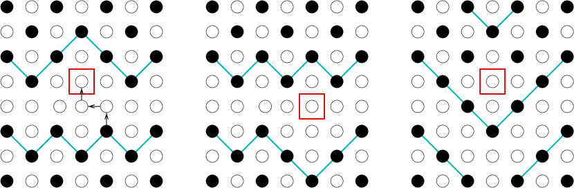
Figure 7: A $6\times 7$ system with a stripe and a hole. The hole is indicated in the box. It is initially lying on the stripe (leftmost state). The arrows indicate the particles hops that result in the hole moving along the stripe to the right (middle state). It is also possible for the stripe to fluctuate and leave the hole immobile (rightmost state).

Motion of holes has been analyzed on domain walls in the anisotropic $t$-$J$ model (the $t$-$J_{z}$ model with some added terms), using essentially analytical techniques. Tch The most interesting observation in Ref. Tch, is that the charge-carrying “holon” is associated with a kink of the wall, and thus carries a transverse “flavor” (reminiscent of our model’s behavior in Sec. IV.4). A hole on our stripe differs in an important way from the holes on a stripe in the $t$-$J_{z}$ model. Tch ; CherNeto00 First, in our case the reference stripe already has 1/2 hole per unit length, whereas in Refs. Tch, and CherNeto00, it is a plain domain wall without holes. Second, $J_{z}/t$ was not too large in those models, so that hopping of the hole several steps away from the stripe has a noticeable contribution in the wavefunction, while it is unimportant in our case.

¿From diagonalization, we observe that for systems with rectangular boundaries, the boson and fermion one-hole-with-a-stripe spectra are identical. The numerical method described in Sec. II.3 is used to check whether the function $\sigma(\alpha)$ is well defined using the state graph Fig. 3. For a $L_{x}\times L_{y}$ system with $L_{x}$ even and $L_{y}$ odd, the one-hole-with-a-stripe state has $M=(L_{x}-1)L_{y}/2-1$ particles. For the one-hole systems we checked, for example, $4\times 9$ with $M=15$, $4\times 11$ with $M=19$, and $6\times 7$ with $M=17$, $\sigma(\alpha)$ is always well defined. Henley-stripehole

IV.1 Energy dependence on $L_{y}$

When a hole is added to a stripe, more hops are allowed and the state gains kinetic energy, so the energy is lower than that of the single stripe of the same length. We define the energy difference,

$$\Delta(L_{x},L_{y})\equiv E_{hole}(L_{x},L_{y})-E_{stripe}(L_{x}),$$ (30)

where $E_{hole}(L_{x},L_{y})$ is the ground state energy of one hole with a stripe on a $L_{x}\times L_{y}$ lattice and $E_{stripe}(L_{x})$ the ground state energy of a single stripe with length $L_{x}$. Here $E_{hole}(L_{x},L_{y})$ is the same for bosons and fermions, as we discussed above, and $E_{stripe}(L_{x})$ does not depend on $L_{y}$ (see Eq. (26)).

A plot of $\Delta(L_{x},L_{y})$ vs $L_{y}$ shows a fast decay in $L_{y}$ so we try the following exponential fitting function,

$$\Delta(L_{x},L_{y})={\tilde{\Delta}}(L_{x})-A(L_{x})e^{-L_{y}/l(L_{x})},$$ (31)

where ${\tilde{\Delta}}(L_{x})=\Delta(L_{x},\infty)$, $A(L_{x})$, and $l(L_{x})$ are fitting parameters that depend on the length of the stripe $L_{x}$. (We will investigate the dependence on $L_{x}$ of ${\tilde{\Delta}}(L_{x})$ later in Sec. IV.3.) We choose a minus sign in front of $A(L_{x})$ because $\Delta(L_{x},L_{y})<{\tilde{\Delta}}(L_{x})$; in Eq. (31), $A(L_{x})$ is positive.

This fitting form Eq. (31), suggests the following linear regression check,

$$\ln(\Delta(L_{x},L_{y}+2)-\Delta(L_{x},L_{y}))=C-\frac{L_{y}}{l(L_{x})},$$ (32)

where $C$ is a constant that depends on $A$, $l$, and $L_{x}$, but not on $L_{y}$. In Fig. 8 we plot $\ln(\Delta(L_{x},L_{y}+2)-\Delta(L_{x},L_{y}))$ vs $L_{y}$ for $L_{x}=4,6,8,10,12,14$ and $L_{y}=5,7,9,...$. The linear fit is excellent for all data sets.

Figure 8: $\ln(\Delta(L_{x},L_{y}+2)-\Delta(L_{x},L_{y}))$ vs $L_{y}$ for $L_{x}=4,6,8,10,12,14$, where $\Delta(L_{x},L_{y})=E_{hole}-E_{stripe}$, Eq. (30). The slope for each $L_{x}$ curve is $-1/l(L_{x})$ in Eq. (32).

IV.2 Stripe potential well and effective mass

How can we account for the exponential fitting form, Eq. (31)? Let us consider the hole fixed at some position and the stripe meandering in $y$ direction. In Fig. 7, we have shown that the hole can be in contact with the stripe or the stripe can fluctuate away, leaving the hole behind and immobile. When the stripe is in contact with the hole, the energy is lower than the energy of a single stripe $E_{stripe}$, which is also the energy when the stripe is separated from the hole. Because we have periodic boundary conditions in the $y$ direction, we can use a periodic array of potential wells to model the $y$ motion of the stripe; the well is at the position of the hole.

Figure 9: Potential-well and barrier potential used to understand the exponential decay of one-hole energy in $L_{y}$ in Eq. (31). $y$ is the stripe position in the direction perpendicular to the stripe, $V_{0}$ is the depth of the well, $E_{0}$ the ground state energy of one isolated well, $E_{2}<E_{0}$ the ground state energy including the tunneling between wells (symmetric state), and $d$ the separation between two wells. $E_{2}-E_{0}$ decays exponentially in $d$ as in Eq. (33).

In Fig. 9 we show potential wells separated by a barrier of thickness $d$. $E_{0}$ is the ground state energy of an isolated well, and $E_{2}$ the ground state energy of the multiple-well system, which corresponds to a symmetric state and is lower than $E_{0}$. From standard quantum mechanics textbooks (see e.g., Ref. Park, ), we know the amplitude to tunnel between adjacent wells difference decays exponentially with their separation,

$$E_{2}-E_{0}=-Ae^{-d/l},\quad\mbox{where,}\quad\frac{1}{l}=\frac{\sqrt{2m(V_{0}-E_{0})}}{\hbar},$$ (33)

where $m$ is the mass of the particle in the well, and the constant $A$ is positive (because the wavefunction of $E_{0}$ is symmetric in one well).

As far as our hole-with-a-stripe problem is concerned, the well separation $d$ is $L_{y}$, the barrier height $V_{0}$ is $E_{stripe}$, the ground state energy of one isolated well $E_{0}$ is $E_{hole}(L_{x},L_{y}=\infty)$, and the ground state $E_{2}$ of the system with tunneling is $E_{hole}(L_{x},L_{y})$. Therefore, Eq. (33) for the wells with tunneling translates into the following equation for our hole-with-a-stripe problem,

$$E_{hole}(L_{x},L_{y})-E_{hole}(L_{x},\infty)=-A(L_{x})e^{-L_{y}/l(L_{x})}.$$ (34)

Using the definition for $\Delta(L_{x},L_{y})$, Eq. (30), we see that Eq. (34) is exactly the fitting form we used before, Eq. (31). In addition, the inter-well tunneling amplitude Eq. (33) gives us a way to calculate the effective mass $m^{*}(L_{x})$ of the stripe of length $L_{x}$,

$$\frac{1}{l(L_{x})}=\sqrt{2m^{*}(L_{x})(E_{stripe}(L_{x})-E_{hole}(L_{x},\infty))},$$ (35)

where we have set $\hbar=1$. We get

$$m^{*}(L_{x})=\frac{1/l^{2}(L_{x})}{2(E_{stripe}(L_{x})-E_{hole}(L_{x},\infty))}.$$ (36)

Using the linear fitting slopes in Fig. 8 (that are $-1/l(L_{x})$), we can compute $m^{*}(L_{x})$ using Eq. (36), and our results are shown in Table 2. The effective mass results are consistent with that obtained from the single-stripe energy dispersion relation in Table 1.

Table 2: Stripe effective mass $m^{*}$ calculated from Eq. (36) using the potential-well model for the one-hole-with-a-stripe problem. $l(L_{x})$ is the decay length in Eq. (31) obtained from linear fitting in Fig. 8; $E_{hole}(L_{x},L_{y})$ is used to approxmate $E_{hole}(L_{x},\infty)$ using the large $L_{y}$ listed in the table (as the exponential decay of $E_{hole}(L_{x},L_{y})$ in $L_{y}$ is fast, see Sec. IV.1); and $m^{*}(L_{x})$ is the effective mass of the length-$L_{x}$ stripe calculated using Eq. (36). $E_{stripe}(L_{x})$ has appeared in Table 1.

$L_{x}$	$L_{y}$	$E_{hole}(L_{x},L_{y})$	$l(L_{x})$	$m^{*}(L_{x})$
4	25	-3.00000009	1.4659	1.3561
6	25	-4.29850460	0.8724	2.2009
8	25	-5.60276427	0.6648	3.0050
10	21	-6.89914985	0.5553	3.7979
12	19	-8.18958713	0.4868	4.5652
14	17	-9.47602246	0.4388	5.3197

The main physical significance of the result in this section is its implications for the anistropic transport of holes in a stripe array. anisotransport ; ZaanenScience The conductivity transverse to the stripes depends completely on mechanisms which transfer holes from one stripe to the next. The high energy of the “stranded” state, in which the hole is immobile and off the stripe, means that holes are mainly transferred when the stripes collide, either directly at contact or else by a delayed transfer, such that the hole spends a short time in a stranded state until the second stripe fluctuates to absorb it.

IV.3 Hole dispersion and $L_{x}$ dependence

In this section we fix $L_{y}$ and study the dependence of $\Delta(L_{x},L_{y})$ on the length of the stripe $L_{x}$. In Fig. 10 we plot the energy difference $\Delta(L_{x},L_{y})$ for $(L_{x},b)\times(0,7)$ systems with $b=0,1,2$.FN-bosonLx

Figure 10: $\Delta(L_{x},L_{y})=E_{hole}-E_{stripe}$ as a function of $1/L_{x}$ for three classes of lattices $(L_{x},b)\times(0,7)$ with $b=0,1,2$.

We see from Fig. 10 the following fitting function (justified in Sec. IV.4) works well for both rectangular and tilted lattices,

$${\tilde{\Delta}}(L_{x})=\Delta+\frac{C(b)}{L_{x}}.$$ (37)

This fitting form enables us to extrapolate the energy gap formed by adding one hole to an infinitely long ($L_{x}$) stripe. The intercepts of the three curves for the three different classes of lattices all approach $\Delta=-0.66$. Later, in Sec. VII.2, we will study the stability of an array of stripes and we will use the value for $\Delta$ because we want to know whether holes added to a stripe stick to the stripe to form a wide stripe or a new stripe. $\Delta$ is energy lowered by adding a hole to a stripe and will be relevant there. It is a binding energy in the sense that one hole off the stripe (immobile) has zero energy.

A hole is mobile along a stripe; one expects its dispersion relation to be

$$E(q)=\Delta+\frac{\hbar^{2}}{2m^{*}_{h}}q^{2}$$ (38)

on a long stripe oriented in the $x$ direction, where $q$ is the hole’s wavevector. We can estimate the effective mass in Eq. (38) from the numerics, if the lowest-energy state with system wavevector ${\bf k}=(q,0)$ is produced by boosting the hole to wavevector $q$. At small $q$, this has a much smaller excitation energy than the ripplons (stripe excitations) which have linear dispersion [Eq. (20)]. Indeed, the numerical spectra for systems with $L_{x}=10$ and $L_{y}=5$ show these contrasting dispersions for a stripe with and without a hole. Fitting the difference $E(q)-E(0)$ to $\hbar^{2}/m^{*}_{h}(1-\cos q)$, as a plausible guess, we estimate $\hbar^{2}/2m^{*}_{h}\approx 0.3t$; the effective mass $m^{*}_{h}$ of a hole bound to a stripe is thus about six times as big as that of a free particle in an empty background (for which $\hbar^{2}/2m^{*}=2t$).

IV.4 Hole and stripe steps

How does the hole interact with the stripe fluctuations? In some models, hole hopping is suppressed if the stripe is tilted away from its favored direction. In that case, the “garden hose effect” is realized: Na97 stripe fluctuations are suppressed when the hole is present, so as to optimize the kinetic energy of the hole on the stripe. FN-Nagaoka

However, in our model, a stripe tilt actually enhances hole hopping. This is clear in the extreme case of a stripe at slope $+1$, as occurs at maximum filling in the $L\times L$ square system with $L$ odd: the bare stripe has zero energy. When the system is doped by placing one hole along an edge of the stripe (see Fig. 11), the accessible configurations are equivalent to a one-dimensional chain of the same model, with length $2L$ and $L-1$ particles on it. The one-dimensional chain has two domain walls, one of which appears as a down-step of the stripe, the other of which appears as an up-step bound to a hole on the stripe. In the limit of large $L$, each domain wall has kinetic energy $-2t$. The total energy is $-4t$, or about seven times larger than the energy difference $-\Delta$ for a stripe with no tilt.

This picture is supported by the trend of the stripe energy with one hole, in the presence of a boundary vector $(L_{x},b)$ that forces a tilt. For $L_{x}=5$ to $8$, the minimum energy, as a function of $b$, occurs around $2.5$. [The measured minimum is at $b=2$ in the case that $L_{x}$ and $b$ are even, at $b=3$ in the odd case, while the second-lowest energies are at $b=4$ and $b=1$, respectively.] This is consistent with the idea that the hole on a stripe binds with some up steps FN-holestep which total $b_{0}$, where $b_{0}\approx 2.5$.

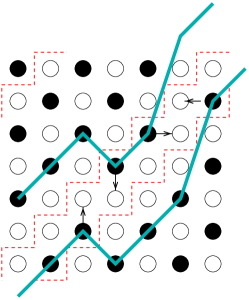
Figure 11: A $7\times 7$ system is shown, at one particle less than maximum filling. All motions in this system occur within the strip bounded by dashed lines, which is equivalent to a $14\times 1$ chain of spinless $V=\infty$ fermions. The stripe edge is indicated by thick solid lines.

This would imply that holes tend to come in “up” and “down” flavors; this is not an actual quantum number, since the “steps” considered here (in contrast to “kinks” mentioned in Sec. III.3.1) are not quantized objects. Our hole-step binding has a similar origin as that in Ref. Tch, : the local configuration is the same as a fragment of stripe rotated $90^{\circ}$ from the main stripe.

A corollary of the hole-step binding is that a hole should force an extra tilt $|b-b_{0}|/L_{x}$ on the remaining portion of the stripe. Thus the tilt energy in Eq. (19) contributes a size dependence $C(b)/L_{x}$, where

$$C(b)=\frac{1}{2}K[(b-b_{0})^{2}-b^{2}]=Kb_{0}(b_{0}/2-b),$$ (39)

that is 4.9, 1.0, and -2.9 for $b=0$, 1, and 2 respectively. This is consistent with the clear $1/L_{x}$ size dependence we found numerically (see Fig. 10); the fitted coefficients for $b=1$ and $2$ are in reasonable agreement with $C(b)$ as predicted by Eq. (39). (Presumably $C(0)$ is reduced from our prediction because the hole is not always, or not usually, bound to an up-step in the case $b=0$.)

V Two Holes on a Stripe

When two holes meet on a stripe, they create enough room that particles can exchange with each other, so the boson and fermion energy spectra are no longer the same. As in the one-hole case, we study the energy of the two-holes-with-a-stripe problem as a function of the two directions of the lattice.

V.1 Energy dependence on $L_{y}$

As in Eq. (30) for the one-hole case, we define for the $L_{x}\times L_{y}$ lattice the energy difference between the case of two holes with a stripe and that of a single stripe,

$$\Delta_{2}(L_{x},L_{y})=E_{2holes}(L_{x},L_{y})-E_{stripe}(L_{x}),$$ (40)

where the subscript 2 denotes the two-hole case. (Strictly speaking, we should write $\Delta_{2}^{b,f}(L_{x},L_{y})$ and $E_{2holes}^{b,f}(L_{x},L_{y})$ because these quantities are not the same for boson and fermion cases. Here, without the superscripts, they stand for both cases.) Plots of $\Delta_{2}(L_{x},L_{y})$ vs $L_{y}$ for bosons and fermions show fast decay similar to that in the one-hole problem in Sec. IV, except here the boson and fermion curves approach different values at large $L_{y}$.

As in Eq. (31) for the one-hole problem, we write

$$\Delta_{2}(L_{x},L_{y})={\tilde{\Delta}}_{2}(L_{x})-A_{2}(L_{x})e^{-L_{y}/l_{2}(L_{x})},$$ (41)

$\ln(\Delta_{2}(L_{x},L_{y}+2)-\Delta_{2}(L_{x},L_{y}))$ vs $L_{y}$ for bosons and fermions have been plotted with $L_{x}=4,6,8,10$. The exponential dependence is checked nicely as in Fig. 8 for the one-hole case, and the slopes are obtained and will be used for calculating the effective mass in the next section.

V.2 Stripe potential well and effective mass

The resemblance of our treatment of the two-holes-with-a-stripe problem in Sec. V.1 with that of the one-hole problem in Sec. IV.1 prompts us to ask whether the two-hole problem can be studied using a one-dimensional effective potential like the potential wells used in Sec. IV.2. Here with two holes, we have a more complicated problem because the relative positions of the two holes and the stripe can have three cases: two holes on the stripe (with energy $E_{2holes}(L_{x},\infty)$), one hole on the stripe with one isolated hole (with energy $E_{1hole}(L_{x},\infty)$), or one stripe with two isolated holes (with energy $E_{stripe}(L_{x})$).

As an approximation, we consider the deepest well ($E_{2holes}(L_{x},\infty)$) only because that is the most probable position to find the particle. Then the effective mass equation Eq. (36) is modified to become,

$$m^{*}_{2}(L_{x})=\frac{1/l^{2}_{2}(L_{x})}{2(E_{stripe}(L_{x})-E_{2holes}(L_{x},\infty))},$$ (42)

where $l_{2}(L_{x})$ comes from the linear fitting slopes. The results for $m^{*}_{2}$ from this two-hole-with-a-stripe calculation are in Table 3. They are comparable to the one-hole results in Table 2.

Table 3: Stripe effective mass $m^{*}_{2}$ calculated from Eq. (42) using the double-well potential model for the two-holes-with-a-stripe problem. $l_{2}(L_{x})$ is the decay length in Eq. (41) obtained from linear fitting. $E_{2holes}(L_{x},L_{y})$ is used to approxmate $E_{2holes}(L_{x},\infty)$ using the large $L_{y}$ listed in the table; and $m^{*}_{2}(L_{x})$ is the effective mass of the length-$L_{x}$ stripe calculated using Eq. (42). The superscripts $b$ and $f$ denote bosons and fermions respectively. $E_{stripe}(L_{x})$ has appeared in Table 1.

$L_{x}$	$L_{y}$	$E_{2holes}^{b}$	$E_{2holes}^{f}$	$l_{2}^{b}$	$l_{2}^{f}$	${m_{2}^{*}}^{b}$	${m_{2}^{*}}^{f}$
4	19	-3.896952	-3.818556	0.5919	0.6135	1.3358	1.3417
6	19	-5.238613	-5.204899	0.4317	0.4386	2.1664	2.1574
8	19	-6.524636	-6.510024	0.3621	0.3643	2.9375	2.9349
10	15	-7.797992	-7.790359	0.3167	0.3274	3.7605	3.5377

V.3 Energy dependence on $L_{x}$ and stripe-step binding

To compare with Fig. 10 for one hole with a stripe, in Fig. 12 we plot $\Delta_{2}(L_{x},L_{y})$, for three classes of lattices $(L_{x},b)\times(0,L_{y}=7)$ with $b=0,1,2$, vs $1/L_{x}$. Here the $1/L_{x}$ fit, as in Eq. (37) for the one-hole problem, is no longer good. But we can still extrapolate the energy gap of the two-hole state and the stripe state for an infinitely long stripe. For the $(L_{x},0)\times(0,7)$ lattices, the gap is extrapolated to be $-1.4$ approximately, for bosons and fermions. Comparing to the single hole gap of $-0.65$, we see that binding between holes are not strong. This information will be useful when we consider stripe-array formation.

Figure 12: $\Delta_{2}(L_{x},L_{y})=E_{2holes}-E_{stripe}$ as a function of $1/L_{x}$ for three classes of lattices $(L_{x},b)\times(0,7)$ with $b=0,1,2$.

The size dependence of two holes on one stripe can be interpreted by the notion (Sec. IV.4) that holes are bound to up- or down-steps. When the boundary vector is $(L_{x},b)$ with $b=0$ or $1$, the stiffness cost will be minimized if the holes adopt canceling flavors “up” and “down” (so long as $b<2b_{0}\approx 5$). This may explain why the $b=0$ curves in Fig. 12 seem to have a weak coefficient of $1/L_{x}$. The fact that $\Delta_{2}\approx 2\Delta_{1}$ indicates weak interaction between the holes, and that can only happen if the holes (of opposite flavors) tend to repel.

However, on reflection it will be noticed that, in a sufficiently large system, added holes can be “condensed” to create segments of stripe oriented in the $\pm\hat{y}$ direction. These “$90^{\circ}$” segments will surely appear in the ground state of one stripe in a large system, as the energy per hole to increase the net stripe length is far lower than the energy to add a free hole hopping along the stripe. Thus, holes do attract, on a sufficiently long stripe. That does not contradict our numerical observation of repulsion: as just explained, the constraint of zero net kink “flavor” on a stripe forces two holes to adopt opposite flavors, which repel, whereas the holes that form a single $90^{\circ}$ segment all have the same flavor.

Two effects compete with the formation of $90^{\circ}$ segments in the case of short stripes or small numbers of added holes: (i) Say the stripe contains one $90^{\circ}$ segment with $h$ holes; that extends $\pm 2h$ (not $\pm b_{0}h$) in the $y$ direction, which forces the remainder of the stripe to have a slope $\mp 2h/L_{x}$ and the associated tilt energy Eq. (19). (ii) Say the stripe contains two $90^{\circ}$ segments, with the opposite directions: no net slope is forced, but twice as many $90^{\circ}$ corners are present, and presumably each $90^{\circ}$ bend costs energy (since it suppresses stripe fluctuations).

The implication is that the $b=0$ and $b=1$ curves in Fig. 12 are heading towards a well-defined asymptote at $-2\Delta_{1}$, corresponding to a pair of repelling, opposite-flavor holes. However, at sufficiently long $L_{x}$, they must cross over to a different curve with a lower asymptote, corresponding to a pair of attracting, same-flavor holes, bound into an incipient $90^{\circ}$ segment. We conjecture that the entire $b=2$ curve is in the latter regime, while the downturn of the $b=1$ curve at the largest $L_{x}$ suggests it is beginning to make the crossover.

VI Two and More Stripes

Starting from this section, we study the interaction among stripes. We use the same diagonalization program for the problem of one stripe and one stripe with holes that was introduced in Sec. II. Again we do not exhaustively enumerate all possible states with a given number of particles $M$. Instead, we build basis states from a starting state which has the stripes all merged together. The motivation of these studies is that understanding of the stripe-stripe repulsion is a prerequisite to calculating the stripe-array energy as a function of filling near $n=1/2$, which in turn is needed in order to ascertain the density at which sthe stripe array would coexist with a liquid phase. Unfortunately, we can only study comparatively short stripes and the asymptotic form for $L_{x}\to\infty$ is quite unsure from our numerical results.

VI.1 Boson and fermion statistics

We observe from exact diagonalization that for rectangular lattices with two stripes, the boson and fermion spectra are identical.FN-close In Fig. 13, we show two configurations of two merged stripes. For a particle on the stripe we see that the horizontal hops are limited by nearest-neighbor replusion to adjacent columns only. This means that, with two stripes, particles cannot move freely along the stripe and the hopping in the system is still primarily in the vertical direction. From Fig. 13, we can also see, after trying some moves, that we cannot move one particle far away enough so as to exchange the position of two particles. This is a necessary condition for the boson and fermion spectra are identical.

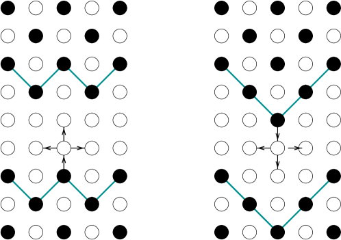
Figure 13: Two configurations of two merged stripes. The arrows indicate the possible hops of one particle along the stripe. The horizontal movement is limited to the adjacent columns only.

We also need to show that periodic boundary conditions do not affect the spectra, and we use again the idea outlined in Sec. II.3. We have, as we did for the one-stripe-with-a-hole problem in Sec. IV, numerically checked a number of systems with two stripes, for example $4\times 10$, $6\times 8$, and $8\times 10$, and we find that for the cases we checked the function $\sigma(\alpha)$ is well defined.

VI.2 Stripe-stripe interaction

¿From diagonalization of two stripes with stripe length $L_{x}=4,6,8$, we observe that the highest-weight states in the ground state eigenvector have stripes far apart from each other, which suggests that stripes may repel. To study the interaction between two stripes quantitatively, we define the following function,

$$\phi^{L_{x}}(d)=\frac{E_{2stripes}(L_{x},L_{y})-2E_{stripe}(L_{x})}{2L_{x}},$$ (43)

where $d$ is the distance between adjacent stripes (here $d=L_{y}/2$ for two evenly spaced stripes), $E_{2stripes}$ the energy of the two-stripe system, and $E_{stripe}$ the energy of one single stripe. $\phi$ is the energy cost per unit length per stripe due to stripe interaction, and it is positive for repelling stripes and negative for attracting stripes. (When we are not considering the dependence of $\phi^{L_{x}}(d)$ on $L_{x}$, we will simply use $\phi(d)$.) In Fig. 14 we show $\phi(d)$ for stripe length 4, 6, and 8. For all cases, $\phi(d)$ is positive (the stripes repel) and decays as the stripe separation $d$ increases. Observe that $\phi(d)$ for $L_{x}=8$ is very much smaller than that for $L_{x}=4,6$. The behavior of $L_{x}=8$, which is not yet explained, is highly significant for extrapolation to the thermodynamic limit. The stripes with $L_{x}=4,6$ were so short that, from Sec. III up to here, their $L_{y}$ size dependence could be explained in terms of a particle moving in one dimension ($y$), completely ignoring their internal fluctuations.

Figure 14: Stripe-stripe interaction energy cost $\phi(d)$ (Eq. (43)) for stripe length 4, 6, and 8. $d$ is the distance between adjacent stripes ($d=L_{y}/2$). The lines are those that connect the data points.

It is clear that as $d\rightarrow\infty$, $\phi(d)\rightarrow 0$ and from the graphs it does not decay exponentially. We try the following power-law fitting function,

$$\phi(d)=\frac{A(L_{x})}{d^{\alpha}}.$$ (44)

In Fig. 15 we plot $\ln(\phi(d))$ vs $\ln(d)$ for $L_{x}=4,6$ with $d=6,8,...,56$, i.e., the largest lattice for $L_{x}=4$ is $4\times 112$ and for $L_{x}=6$ is $6\times 112$. We see that the power-law assumption is good for $L_{x}=4$ with the decay exponent $\alpha$ (slope in Fig. 15) close to 2. For $L_{x}=6$ we observe that the slope approaches 2 as the stripe separation $d$ is large.

Figure 15: log-log plot of energy cost function $\phi(d)$ (Eq. (43)) for stripe length $L_{x}=4,6$, with $d=6,8,...,56$. The slope (decay exponent $\alpha$ in Eq. (44)) is close to 2 for $L_{x}=4$, and for $L_{x}=6$ the slope approaches 2 as stripe separation $d$ increases. Linear regression is used for all $L_{x}=4$ data, and for the $L_{x}=6$ data, only the ten points with the largest $d$ are used.

VI.3 Power-law decay and stripe effective mass

In Sec. IV.2, we explained the exponential decay of the one-hole-with-a-stripe energy in $L_{y}$ by mapping the stripe motion to a one-dimensional problem with a double-well potential. Here with two stripes in the system, we have shown again that stripe fluctuations as a function of $x$ are limited, and we expect a one-dimensional potential can be sufficient in capturing the essential physics.

Here we consider the two stripes as hard-core particles of mass $m^{*}$ moving in the $y$ direction only. This can be mapped to a pair of fermions on a one-dimensional ring of length $L_{y}$, mathematically just like the one-dimensional fermions of Sec. III.4, that move in the $x$ direction, but with a completely different relation to the physics. FN-reducedmass The wavevectors of these one-dimensional fermions are thus $\pm\pi/L_{y}$, so the total energy is

$$E=\frac{\hbar^{2}}{2m^{*}}2\left(\frac{\pi}{L_{y}}\right)^{2}=\frac{\hbar^{2}\pi^{2}}{m^{*}L_{y}^{2}}.$$ (45)

For the two-stripe problem, from curve fitting in Fig. 15, the decay exponent $\alpha$ is close to 2 for $L_{x}=4$. Using Eq. (44) for $\phi(d)$, the definition for $\phi(d)$ in Eq. (43), and $d=L_{y}/2$ for two evenly spaced stripes, we have the following formula for the two-stripe interaction energy

$$E_{2stripes}-2E_{stripe}=\frac{8L_{x}A}{L_{y}^{2}},$$ (46)

where $A$ is the factor in Eq. (44).

Eqs. (45) and (46) give an expression for the effective mass of a stripe from two-stripe interaction,

$$m^{*}(L_{x})=\frac{\pi^{2}}{8L_{x}A}.$$ (47)

The linear fitting intercept in Fig. 15 gives, for $L_{x}=4$, $A=\exp(-1.596418)$, and Eq. (47) then gives us the effective mass $m^{*}(4)=1.5222$. In Table 2, the $L_{x}=4$ stripe effective mass calculated in the one-hole-with-a-stripe problem is 1.3561, and in Table 3 that from the two-hole problem is 1.3417 for fermions and 1.3358 for bosons. All these results for the effective mass of a short, length-four stripe are comparable.

It is clear that the shorter the stripes the better the one-dimensional approximating model is. For $L_{x}=6$, it can be seen in Fig. 15 that the exponent approaches 2 in the large-$d$ limit, but for $d$ close to 56 (the largest system that we calculated), linear regression still gives 1.91. The intercept for $L_{x}=6$ in Fig. 15 is not yet sufficient for us to use Eq. (47) to calculate the stripe effective mass.

VI.4 Three and four stripes

We have also studied the interaction of three and four stripes with stripe length $L_{x}=4$. From diagonalization, we find that for 2, 3, and 4-stripe fermion systems we computed, the ground state energy always appears in the ${\bf k}=(0,0)$ sector, and the highest-weight states in the ground state eigenvector have stripes far apart. To study the interaction of three stripes, we define, in the same fashion as Eq. (43), the energy cost per unit length per stripe,

$$\phi_{3}(d)=\frac{E_{3stripes}(L_{x},L_{y})-3E_{stripe}(L_{x})}{3L_{x}},$$ (48)

where $d=L_{y}/3$ here. In Fig. 16 we plot $\phi_{3}(d)$ vs $d$ and $\ln(\phi_{3}(d))$ vs $\ln(d)$. First of all, with three or more stripes, unlike the two-stripe case, particles have enough room to exchange with each other when the stripes merge, and the fermion and boson energies are no longer the same.FN-phi3 (However, we see from the graph that the boson and fermion energies are only slightly different.) It is clear that the stripes repel and the exponent of $\phi_{3}(d)$ for $L_{x}=4$ is 2.004 for the boson case (and practically the same for the fermion case, not shown in the graph), close to 1.983, the exponent for the two-stripe $L_{x}=4$ case (see Fig. 15).

Figure 16: Stripe-stripe interaction energy cost $\phi_{3}(d)$ (Eq. (48)) for three stripes with length 4 ($L_{x}=4$). $d$ is the distance between adjacent stripes ($d=L_{y}/3$). The boson and fermion energies are slightly different. The log-log plot is shown below, showing for bosons an exponent $2.004$.

The stripes are short enough in the $x$ direction to be treated as rigid (See Sec. III). They are, in effect, three hardcore particles moving in one dimension. Apart from the fact that this one dimension runs along $y$, exactly the same problem was studied in Sec. III.3, where we recalled that it is convenient to convert such particles to fermions.

Let us consider the ground state of three fermions of mass $m^{*}$ in a length-$L_{y}$ box. They have wavevectors $q_{y}=0$ and $\pm 2\pi/L_{y}$, so the total energy is

$$E=\frac{\hbar^{2}}{2m^{*}}\left(0+2\left(\frac{2\pi}{L_{y}}\right)^{2}\right)=\frac{4\pi^{2}/m^{*}}{L_{y}^{2}}.$$ (49)

For the three-stripe problem, we use the same $1/d^{2}$ relation for $\phi_{3}(d)$, as in Eq. (44) for the two-stripe problem,

$$\phi_{3}(d)=\frac{A_{3}(L_{x})}{d^{2}},$$ (50)

where $A_{3}(L_{x})$ is a constant. Rearranging Eqs. (49) and (50) gives us a formula for stripe effective mass $m^{*}(L_{x})$, similar to the two-stripe formula in Eq. (47),

$$m^{*}(L_{x})=\frac{4\pi^{2}}{27L_{x}A_{3}(L_{x})}.$$ (51)

Using the linear fitting intercept in Fig. 16, we get for $L_{x}=4$, $A_{3}(4)=\exp(-1.394246)$, and then from Eq. (51), we get $m^{*}(4)=1.4738$, which is consistent with the two-stripe result $1.5222$ calculated in Sec. VI.3.

We have also calculated the energy for the smallest system with four stripes: the $4\times 12$ system with 16 particles. Here the boson energy is $-10.8525$ and the fermion energy $-10.8418$, both higher than the energy of four indepedent stripes with length 4, $-11.3137$.

VII The Stripe-array

In this paper, we have studied the limit near the half-filled, checkerboard state, with cases of a single stripe, holes-on-a-stripe, and a few stripes. As we approach intermediate fillings, around 1/4, we could have two situations: the separation of the system into particle-rich and hole-rich regions (sometimes argued to be quite general for interacting fermions with short-range interactions visscher ; Emery90 ) or else an array of stripes. How do we know which state is the ground state for our model? How do we know whether the stripe-array state is stable?

If the true behavior, in the thermodynamic limit, is phase separation between the half-filled checkerboard state and a hole-rich liquid, then – in a sufficiently large finite system – the ground state would consist of one large (but still immobile) droplet in a checkerboard background, of the sort explained in Subsec. II.2.1. However, in the smallish systems tractable by exact diagonalization, the ground state would probably be a stripe-array state, for (as we find in Sec. VII.2), the bulk energy density difference is quite small between the stripe-array state and the phase-separated state, yet the latter state must pay a considerable extra cost of the phase-boundary line tension times the droplet’s perimeter.

On the other hand, the stripe-array state in a finite system is extremely sensitive to boundary conditions: the concentration of holes may be just right to form one stripe across the system, but if the boundary vectors are both even, the system can only support an even number of stripes. Even if the stripe-array is the correct thermodynamic answer at this hole filling, the best state available to this finite system is a separated droplet.

We conclude that one cannot accept the behavior of our finite systems as a direct picture of the thermodynamic limit, because finite systems are dominated by finite-size and topological effects. The correct approach is to determine the equation of state for each competing phase by extrapolating it to the thermodynamic limit, and only then to perform a Maxwell construction to determine the phase stability. Note that different extrapolation schemes may be appropriate for qualitatively different phases.

VII.1 Stripe-array chemical potential

We first calculate the chemical potential of the stripe-array, i.e., the energy per hole in creating a new stripe; this information will be needed for stability analysis later. We have previously presented this calculation in a condensed form.HenleyZhang

Say we have a $L_{x}\times L_{y}$ system with $p$ stripes stretching in the $x$ direction. The number of particles per column is $(L_{y}-p)/2$ and the total number of particles is $M=(L_{y}-p)L_{x}/2$. Denote the total number of lattice sites $N=L_{x}L_{y}$, then the particle density is

$$n=\frac{M}{N}=\frac{1}{2}-\frac{p}{2L_{y}}=\frac{1}{2}-\frac{1}{2d},$$ (52)

where $d$ is the separation between adjacent stripes and for even distributed stripe we have $d=L_{y}/p$. We then have $d=1/(1-2n)$.

The energy of the stripe-array has two contributions: the energy from indepedent stripes and the energy due to stripe-stripe interaction. The energy per length $\sigma_{0}$ of an infinitely long stripe is $\sigma_{0}=-2/\pi$, which can be obtained from mapping the stripe to the spin-1/2 chain.Mila Therefore the energy of $p$ independent stripes is

$$E_{indep}=p\,\sigma_{0}L_{x}=\frac{\sigma_{0}}{d}L_{x}L_{y},$$ (53)

where we have used $p=L_{y}/d$. On the other hand, the energy due to stripe-stripe interaction is

$$E_{interaction}=p\,\phi(d)L_{x}=\frac{\phi(d)}{d}L_{x}L_{y},$$ (54)

where we have used the two-stripe interaction energy per length per stripe $\phi(d)$ defined in Eq. (43). (Note that we have seen in Sec. VI.2 that $\phi$ also depends on the length of the stripe $L_{x}$. Fortunately, in the following, we will only work in the $d\rightarrow\infty$ limit of $\phi(d)$, which is independent of $L_{x}$.) Combining Eq. (53) and Eq. (54), we obtain the energy density of the stripe array as a function of particle density $n$,

$${\cal E}_{sa}(n)=\frac{E_{indep}+E_{interaction}}{N}$$

$$=(\sigma_{0}+\phi(d))\frac{1}{d}=(\sigma_{0}+\phi(d))(1-2n).$$ (55)

Furthermore, we have seen, when we studied stripe-stripe interaction, $\phi(d)$ is positive and $\phi(d)\rightarrow 0$ as $d\rightarrow\infty$. So in the infinite-lattice limit we have

$${\cal E}_{sa}(n)=\sigma_{0}(1-2n).$$ (56)

That is to say that the chemical potential of the stripe-array is

$$\mu^{*}=\frac{d{\cal E}_{sa}(n)}{dn}=-2\sigma_{0}=\frac{4}{\pi}=1.273,$$ (57)

where the result for $\sigma_{0}$ is used. Eq. (57) says that the slope of the stripe energy density curve is $1.273$, and if we have an array of stripes in the system then adding a particle to the system will raise the energy by $1.273$, or equivalently, adding a hole to the stripe-array will lower the energy by $1.273$. This is an important quantity in the stability analysis that is to follow.

VII.2 Stripe-array stability

We consider three stability conditions for the stripe-array agains phase separation.

VII.2.1 Stability condition 1: stripes repel

We have already studied stripe-stripe interaction, and we know that stripes repel (see Fig. 14 for example). This is our first stability condition.

VII.2.2 Stability condition 2: two stripes beat one fat stripe

Our second stability condition comes from the work on the one-hole-with-a-stripe problem in Sec. IV.3. Here we want to know whether with more holes new stripes will form or the existing stripes just get wider (thus leading to phase separation). We showed in Sec. IV.3 that adding a hole to an infinitely long stripe lowers the energy by 0.66. Here we have shown that adding a hole to a stripe-array lowers the energy by 1.273. The stripe-array state is therefore preferred.

VII.2.3 Stability condition 3: stripe-array beats phase separation

The third stability condition comes from free energy analysis in statistical mechanics. Here because we are considering zero temperature physics and $F=E-TS$, energy is free energy. In Fig. 17 we show the two cases. The dashed tie-line is the Maxwell construction. It is tangent to the liquid curve (small fillings) and is connected to the half-filled state at $n=1/2$. It represents the coexistence of the liquid state and the half-filled state, i.e., the phase separated state. According to Sec. VII.1, the stripe-array line should have slope 1.273, and it is drawn from the half-filled limit. The stripe-array case is stable when the stripe-array line is below the dashed line, otherwise the phase separated state is stable. Therefore, to determine the stability of the stripe-array against phase separation, we need to determine the slope of the dashed line $\mu^{\rm LC}$. Here we are following the notation in Ref. HenleyZhang, and the superscript LC denotes the two states: liquid and CDW (charge-density-wave, i.e., half-filled state) that are connected by the dashed line.

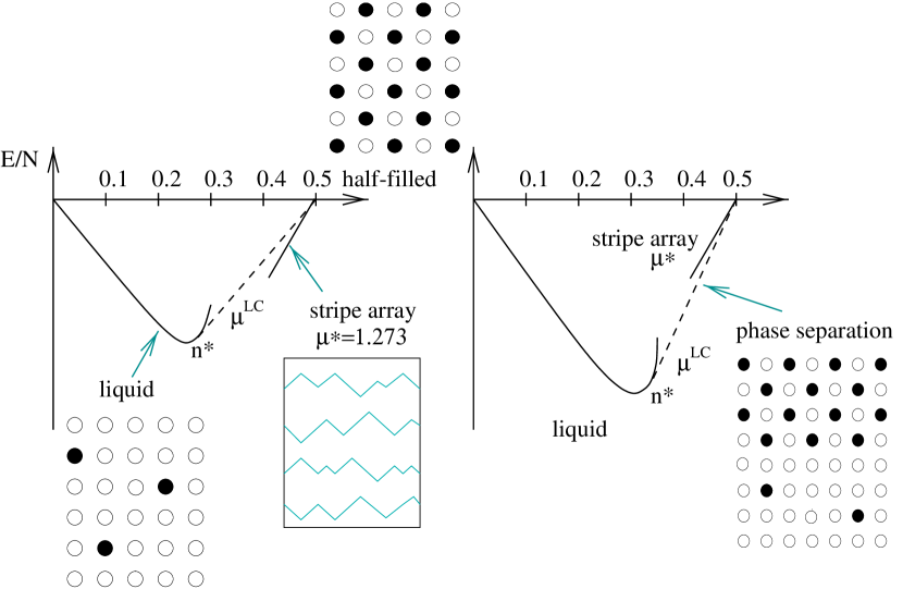
Figure 17: Stability of the stripe-array vs phase separation. Energy density $E/N$ vs particle density $n=M/N$. The stripe-array curve has slope $\mu^{*}=1.273$. The dashed line is tangent to the liquid curve and is connected to the half-filled state. It represents the coexistence of the two phases: liquid and half-filled states, i.e., a phase separated state. On the left is the case where the stripe-array line is below the dashed line, and therefore the stripe-array is stable. On the right is the case where the dashed line is below the stripe-array line, i.e., the phase separated state is stable. $n^{*}$ is the intersection of the tie-line with the liquid curve, and the key quantity is the slope of the dashed line $\mu^{\rm LC}$.

To obtain $\mu^{\rm LC}$, we need a fitting function for the energy density $E/N$ at intermediate fillings (the liquid part). We use a polynomial form, up to the third order in particle density $n=M/N$,

$${\cal E}(n)=\frac{E(n)}{N}=A_{1}n+A_{2}n^{2}+A_{3}n^{3},$$ (58)

where $E(n)$ is the energy of the $M$ particle system. We should emphasize that this fitting form Eq. (58) is not meant for the dilute limit ($n\rightarrow\infty$). This is for the intermediate-filling, with $n\approx 1/4$. Eq. (58) can also be written as

$$\frac{E}{M}=A_{1}+A_{2}n+A_{3}n^{2},$$ (59)

where $E/M$ is the energy per particle. We will use Eq. (59) to fit diagonalization results. The slope $\mu^{\rm LC}$ can be determined by first solving for $n^{*}$, the $n$ coordinate of the intersection of the dashed tie-line with the liquid curve, using

$$\mu^{\rm LC}=\frac{{\cal E}(n^{*})-0}{n^{*}-1/2}=\frac{d{\cal E}(n)}{dn}\Bigg{|}_{n^{*}}.$$ (60)

Figure 18: Fermion (top) and boson (bottom) $E/M$ vs $n=M/N$ fit for intermediate fillings ($0.19\leq n\leq 0.31$). The fermion data have larger spread than the boson data because of the fermion shell effect

In Fig. 18, we plot, for fermions and bosons, $E/M$ vs $n$ at the intermediate fillings ($0.19\leq n\leq 0.31$) for a number of lattices with lattice size ranging from 25 to 42.FN-lattices In Table 4 we list the quadratic fitting parameters obtained from diagonalization data. For the ten lattices in Fig. 18, using Eq. (60), we obtain ${\mu^{\rm LC}}=1.254$ for fermions and ${\mu^{\rm LC}}=1.304$ for bosons.

Table 4: Fermion and boson fitting parameters (in Eq. (58)) and the calculated $n^{*}$ and ${\mu^{\rm LC}}$ (using Eq. (60)), for all ten lattices in Fig. 18 and for the smallest and largest five lattices separately. Compared with the stripe-array slope $\mu^{*}=1.273$, the fermion stripe-array is stable against phase separation (${\mu^{\rm LC}}<\mu^{*}$), and the boson stripe-array is unstable (${\mu^{\rm LC}}>\mu^{*}$).

Particle	Lattice	$A_{1}$	$A_{2}$	$A_{3}$	$n^{*}$	${\mu^{\rm LC}}$	SA Stable?
Fermion	all 10	-5.454	23.597	-27.186	0.251	1.254	Stable
	small 5	-5.995	28.230	-36.825	0.255	1.240
	large 5	-5.102	20.586	-20.932	0.250	1.264
Boson	all 10	-6.138	27.839	-33.950	0.233	1.304	Unstable
	small 5	-6.378	29.929	-38.420	0.231	1.301
	large 5	-5.994	26.580	-31.251	0.233	1.307

In Table 4, we have also included calculations for the five smallest and five largest lattices in Fig. 18 separately. We find that ${\mu^{\rm LC}}$ for both boson and fermion increases with increasing lattice size. For the boson case, this means that for large lattices, the stripe-array is not stable against phase separation (${\mu^{\rm LC}}>\mu^{*}=1.273$). For the fermion case, the result is stable (${\mu^{\rm LC}}<\mu^{*}$) for the lattices that we have studied, but ${\mu^{\rm LC}}$ is very close to the stability limit 1.273. The fermion stripe-array is possibly stable.

In our earlier publication, Ref. HenleyZhang, , we used the same polynomial fitting function, Eq. (58), but we fixed $A_{1}=-4$, corresponding to the energy of an noninteracting particle, and our systems there went from 20 sites ($4\times 5$) to 36 sites ($6\times 6$). The analysis in this section and the results in Table 4 are obtained using the three-parameter ($A_{1},A_{2},A_{3}$) fit for bigger lattices, from 25 sites ($5\times 5$) to 42 sites ($6\times 7$). The conclusion in Ref. HenleyZhang, was ${\mu^{\rm LC}}=1.25(2)$ for fermions, and ${\mu^{\rm LC}}=1.33(2)$ for bosons.

Ref. hebertbatrouni, simulated the boson case of our model Eq. (1), using Quantum Monte Carlo, but with $V<\infty$. Their phase diagram, Fig. 11 of Ref. hebertbatrouni, , shows a first-order phase transition between the $(\pi,\pi)$ solid [i.e. the checkerboard phase] and a superfluid [the hole-rich phase with $n\leq 0.25$. Our results correspond to a single point $(t/V,\mu/V)=(0,0)$ on their plot; however, their phase boundary approaches that point with a slope batrouni-private $2.28$, i.e. at $\mu/t=2.28$ in the $V\to\infty$ limit, or $\mu/t=2.4$ in a related simulation. troyer . This is much larger than our result $\mu_{\rm LC}\approx 1.33$. That is puzzling, since it would imply either that the liquid state (with density $n\approx 0.25$) has much lower energy than we found, or else that a state exists at $n\approx 0.4$ (in these finite systems) having much lower energy than the stripe states we studied.

The evidence in Ref. hebertbatrouni, for phase separation rests on histograms such as their Fig. 10 which exhibits (for $V=2.86$ in an $8\times 8$ system) a bimodal probability distribution for the density $n$, in a grand canonical ensemble, with peaks at $n=0.5$ (the checkerboard state) and $n\approx 0.39$, the latter being interpreted as a liquid state. For our $V=\infty$ model, a similar plot at low temperature would show peaks at $n=0.5$ and at $n=0.375$. The latter peak represents a two-stripe state with 8 holes. Its energy is $\approx-8\sqrt{1+1/\sqrt{2}}$ $\approx-10.45$ (using Eq. (26), and neglecting the stripe-stripe interaction in light of Fig. 14). Our point is that examination of the most probable configurations is needed in order to judge whether the coexisting state contains stripes or liquid droplets. Indeed, the discrete coexistence between $n=0.5$ and $n=0.375$ is an artifact of the periodic boundary conditions – in the thermodynamic limit, within the stripe-array phase, density $n$ varies continuously with the chemical potential.

VIII Conclusion

VIII.1 Summary

In this paper we studied systematically a two dimensional model of strongly-interacting spinless fermions and hardcore bosons on the square lattice Eq. (1) near the half-filled limit. We considered an extended, quantum-fluctuating object that is natural in our model at the dense limit–the stripe. After introducing our model (Sec. I) and our diagonalization program (Sec. II), we made a detailed study of the problems of a single stripe (Sec. III), up to two holes on a stripe (Secs. IV and V), stripe-stripe interaction of two, three, and four stripes (Sec. VI), and finally the stability of an array of stripes (Sec. VII). Our theoretical studies were aided with substantial amount of results obtained from exact diagonalization.

As is well-known, quantum systems in two dimensions are much more difficult to study than those in one dimension. Because of the presence of strong repulsion, at the dense limit of our model, motion is severely limited. We showed that for the problems of a single stripe, holes on a stripe and a few stripes, analytical results can be obtained by mapping the two-dimensional problems to one-dimensioinal ones, which can in turn be studied using the analytical tools available in one dimension. We showed in great detail the intricacies of each map, including for example, the many-to-one problem, the resulting phase factors, and the role of boson and fermion statistics.

Another theme in this paper is the comparison between the boson and fermion problems. At the center of this comparison is the state graph introduced in Sec. II which describes graphically the relationship among the basis states. For the problems of a single stripe, holes on a stripe, and a few stripes, we investigated the effect of particle statistics on eigenenergy, with the help of the state graph and our computer program. And for the problem of stripe-array stability, we obtain from diagonalization results an interesting conclusion that the boson stripe-array is not stable and the fermion stripe-array is very close to the stability limit and is possibly stable.

This paper taken as a whole is an attempt to understand stripes as macroscopic objects arising from microscopic components (the spinless fermion and hardcore boson particles in our model). The underlying physics is the quantum mechanics of the component particles that is described by a many-particle Schrodinger equation (which we solve by exact diagonalization). Stripes can perhaps be called an emergent phenomenon and are results of collective motions of many microscopic particles (the original particles or holes). They can perhaps be considered in the same fashion as phonons arising from collective lattice vibrations. And like phonons, the stripes in our problem have a life of their own, and we have tried, in this paper, to understand the new physics they bring.

This paper is one of the first using exact diagonalization to study stripes. This is possible because of the significant Hilbert space reduction afforded by our model Eq. (1), spinless fermions and hardcore bosons with infinite nearest-neighbor repulsion. We believe that this is one of the simplest microscopic lattice model with which to study stripes from the underlying particle dynamics. And as we commented in our other paper on the dilute limit of this model,dilutepaper this model deserves to be better known and better studied.

VIII.2 Future directions

There are a number of directions in which the work of this paper might be extended. For example, our code handles quite arbitrary periodic boundary conditions, not necessarily rectangular or square. Our key use of this feature was to accurately measure the equation of state for the strongly interacting liquid at density $n\approx 0.25$, as used in Sec. VII.2 to decide the stripe-array stability. By including a wide variety of differently shaped fermion systems in Fig. 18 (top plot), in effect we average out the “noise” (which is due to fermion shell effects dilutepaper ). An alternative way to do the same thing, which we have not implemented in the present work, would be to impose a phase factor across the boundary conditions and average over all phases. phasetwist

A boundary condition could be used to investigate the 90^∘ bend of a stripe, which was discussed in Sec. V.3. These would force a diagonal stripe, as in Fig. 11, but additional holes would be added to the stripe which are expected to condense and form a segment at right angles. That geometry would permit estimation of the energy cost of the $90^{\circ}$ bend.

This study has focused entirely on eigenenergies; since our diagonalizations provide the wavefunctions too, we could have computed a variety of informative expectations, such as correlation functions. We did make qualitative observations using snapshots of the high-weighted configurations. In our diagonalizations with two or more stripes (Sec. VI.4), which started from a state with stripes all merged, the highest-weight state in the ground state eigenvector has stripes far apart from each other, and nearly equally spaced, as expected from the one-dimensional approximate wavefunctions of Sec. VI. Calculation of the probability distribution for the stripe separation would provide a quantitative test of those wavefunctions. Similar calculations would give a more direct check of the exponential decay of the hole probability as a function of its distance from a stripe, as predicted in Sec. V.2; and would immediately reveal the attractive or repulsive tendency of two holes on a stripe (Sec. V.3).

We studied the case of one stripe with two holes; the case of two stripes with one hole is also worth investigating. The finite-size dependence of the extra energy due to the hole would shed light on the processes by which the hole is transferred between stripes when they touch. Such processes are critical to the transport properties of the stripe array, as considered in Refs. anisotransport, in the spinfull case.

Up to here, we discussed further kinds of measurements which could be made on the same model system; variations are also possible of the model itself. The most obvious of these is to treat $V<\infty$. A large but finite $V$ may be handled in the spirit of the $t$-$J$: the same highly restricted basis states (which facilitated our diagonalizations) are retained, but new hopping terms along [2,0] and [1,1] type vectors appear, with amplitudes $-t^{2}/V$, wherever the intervening site would be forbidden by the nearest-neighbor exclusion. It is not obvious whether this tends to stabilize or to destabilize the stripe array. The inclusion of another form of correlated hopping (Ref. HenleyZhang, , Fig. 3(c)) can certainly stabilize or destabilize the stripe array depending on its sign. HenleyZhang

Finally, the same code is adaptable, almost without modifications, to the triangular lattice. That may model ³He or ⁴He atoms adsorbed on graphite or on carbon nanotubes, green00 ; green02 which implement a periodic boundary condition in one direction.

Appendix A Counting basis states for the program

We find the number of basis states ${\cal N}$ is maximum for fillings $n\equiv M/N\approx 0.25$, close to the filling $n^{*}$ at which, in the thermodynamic limit, (see Sec. VII.2) a hole-rich liquid coexists with the half-filled state or the (nearly-half-filled) stripe array state. This count may be estimated by adapting Pauling’s trick for the ice model entropy Pauling . The number of ways merely to distribute $M$ particles over $N$ sites, uncontrained, is ${N\choose{M}}$ implying the usual entropy $-n\ln n-(1-n)\ln(1-n)$ as $N\to\infty$; this must be corrected to account for the constraint of no nearest neighbors. One chosen particle has a probability $(1-n)^{4}$ to be free of nearest neighbors. If we pretend this event is independent as each particle on (say) the even lattice is chosen in turn, then the $M/2$ power of this probability is the chance for the whole configuration to be valid. The net entropy is estimated as $-n\ln n-(1-3n)\ln(1-n)$; this attains its maximum $0.42$ around $n=0.24$. implying the leading dependence ${\cal N}\sim 1.54^{N}$ for the $V=\infty$ spinless case, compared to ${\cal N}\sim 4^{N}$ in the Hubbard model case. In fact, for a $7\times 7$ lattice, the block with $M=11$ particles has the largest (translation-reduced) matrix dimension, ${\cal N}=1906532$.

Let ${\cal N}^{s}_{h}(L_{x},L_{y})$ be the number of basis states (per ${\bf k}$ vector) in a configuration with $s$ stripes and $h$ holes on it. This grows exponentially with $L_{x}$ but comparatively slowly with $L_{y}$, so we can handle quite large $L_{y}$, and moderately large $L_{x}$.

In the case of one stripe, the map to an XX spin chain (Sec. III.2) makes clear that, independent of $L_{y}$, the basis has $\sim{L_{x}}^{-1}{{L_{x}}\choose{L_{x}/2}}$ states (where ${A\choose B}\equiv A!/[B!(A-B)!]$). Asymptotically ${\cal N}^{1}_{0}(L_{x},L_{y})\sim 2^{L_{x}}/{L_{x}}^{3/2}$.

The number of states with two stripes may be estimated by placing them independently – the correction from disallowing overlaps is subdominant. That is the square of the one-stripe count, multiplied by $L_{x}L_{y}$ for the possible vectors offsetting one stripe relative to the other, i.e. ${\cal N}^{2}_{0}(L_{x},L_{y})\sim 2^{L_{x}}/{L_{x}}^{3/2}$. $\sim 4^{L_{x}}L_{y}/L_{x}^{2}$.

For one stripe with one hole, the basis states were counted for $L_{y}\leq 25$ and $L_{x}\leq 10$. Empirically,

$${\cal N}^{1}_{1}(L_{x},L_{y})=\frac{1}{2}{{L_{x}}\choose{L_{x}/2}}(L_{y}-1)+B(L_{x})$$ (61)

exactly, where $B(4)=-2$, $B(6)=-4$, $B(8)=-8$, $B(10)=-14$; for $L_{y}=7$, this appears to follow with $B(12)=-12$, $B(14)=66$, $B(16)=572$. The linear increase with $L_{y}$ is due to the states with the hole away from the stripe.

For a stripe with two holes, Eq. (61) gets multiplied by an additional factor $L_{x}L_{y}$, for the possible offset of the second hole relative to the first. Empirically, ${\cal N}^{1}_{2}(6,L_{y})=15{L_{y}}^{2}-47L_{y}+4$ (valid for $L_{y}>L_{x}$); this is inferred from $L_{y}\leq 19$. For $L_{y}=7$, we found roughly ${\cal N}(L_{x},7)\sim 3.5{L_{x}}^{1/2}2^{L_{x}}$, for $L_{x}$ up to 13.

References

- (1) J. M. Tranquada, D. J. Buttrey, V. Sachan, and J. E. Lorenzo, Phys. Rev. Lett. 73, 1003 (1994); J. M. Tranquada, B. J. Sternlieb, J. D. Axe, Y. Nakamura, and S. Uchida, Nature 375, 561 (1995).
- (2) J. Zaanen, Science 286, 251 (1999).
- (3) V. J. Emery, S. A. Kivelson, and J. M. Tranquada, Proc. Natl. Acad. Sci. USA 96, 8814 (1999).
- (4) S. R. White and D. J. Scalapino, Phys. Rev. Lett. 80, 1272 (1998).
- (5) S. R. White and D. J. Scalapino, Phys. Rev. Lett. 81, 3227 (1998).
- (6) J. Zaanen Phys. Rev. Lett. 84, 753 (2000).
- (7) H. Q. Lin and J. E. Gubernatis, Comp. Phys. 7, 400 (1993).
- (8) N.-G. Zhang and C. L. Henley, to be submitted to Phys. Rev. B.
- (9) W. Kohn, Phys. Rev. Lett. 19, 789 (1967).
- (10) G. S. Uhrig and R. Vlaming, Phys. Rev. Lett. 71, 271 (1993); G. S. Uhrig and R. Vlaming, Physica B 206 & 207, 694 (1995).
- (11) J. K. Freericks, Phys. Rev. B 47, 9263 (1993).
- (12) R. Lemanski, J.K. Freericks, and G. Banach, preprint (cond-mat/0204503).
- (13) The system Ba1-xKxBiO3 is argued to have stripes of that sort, by I. B. Bischofs, P. B. Allen, V. N. Kostur, and R. Bhargava, preprint (cond-mat/0203486).
- (14) R. A. de Groot, F. M. Mueller, P. G. van Engen, and K. H. J. Buschow, Phys. Rev. Lett. 50, 2024 (1983); V. Yu. Irkhin and M. I. Katsnel’son, Physics-Uspekhi 37, 659 (1994) [Usp. Fiz. Nauk 164, 705-24 (1994)].
- (15) J. R. Cullen and E. Callen, Phys. Rev. Lett. 26, 236-8 (1971).
- (16) J.-H. Park, E. Vescovo, H.-J. Kim, C. Kwon, R. Ramesh, and T. Venkatesan, Nature 392, 794 (1998).
- (17) H. Seo, M. Ogata, and H. Fukuyama, Phys. Rev. B 65, 085107 (2002).
- (18) See, e.g., E. Manousakis, preprint (cond-mat/0201142).
- (19) D. Green and C. Chamon, Phy. Rev. Lett. 85, 4128 (2000).
- (20) D. Green and C. Chamon, preprint (cond-mat/0105250).
- (21) Ref. Pre93, did investigate the tendency, as a function of , for four holes to line up [stripe-like correlation] in the typical configurations found in exact diagonalizations of the - model on up to 20 sites.
- (22) J. Zaanen, J. Phys. Chem. Solids 59, 1769 (1998).
- (23) S. R. White and D. J. Scalapino, preprint (cond-mat/0006071).
- (24) G. Baskaran, Mod. Phys. Lett. B 14, 377 (2000).
- (25) V. J. Emery and S. A. Kivelson, Physica C 209, 597 (1993); V. J. Emery, S. A. Kivelson, and O. Zachar, Physica C 282, 174 (1997).
- (26) J. Zaanen, M. L. Horbach, and W. van Saarloos, Phys. Rev. B 53, 8671 (1996).
- (27) H. Eskes, R. Grimberg, W. van Saarloos, and J. Zaanen, Phys. Rev. B 54, R724-7 (1996); H. Eskes, O. Y. Osman, R. Grimberg, W. van Saarloos, and J. Zaanen, Phys. Rev. B 58, 6963 (1998).
- (28) C. Morais Smith, Yu. A. Dimashko, N. Hasselmann, and A. O. Caldeira, Phys. Rev. B 58, 453 (1998).
- (29) O. Tchernyshyov and L. P. Pryadko, Phys. Rev. B 61, 12503 (2000).
- (30) A. L. Chernyshev, A. H. Castro Neto, and A. R. Bishop, Phys. Rev. Lett. 84, 4922 (2000).
- (31) L. P. Pryadko, S. Kivelson, and D. W. Hone, Phys. Rev. Lett. 80, 5651 (1998); L. P. Pryadko, S. A. Kivelson, V. J. Emery, Y. B. Bazaliy, and E. A. Demler, Phys. Rev. B 60, 7541 (1999).
- (32) This phase separation is between the half-filled phase and a stripe-array (still near half-filling) with a particular spacing . It is not the phase separation, involving a hole-rich phase, that we (or Ref. Emery90, ) have been concerned with. (Note in Ref. Pryadko98, the roles of long- and short-range forces are reversed from Ref. Emery90, , as to which kind produces phase-separation and which produces a stripe array.) One should also note that Ref. Pryadko98, models stripes as fixed. Its conclusion is not guaranteed for the case, closer to the cuprates, that the frequency scale of stripe fluctuations, , exceeds that of spin waves, .
- (33) P. Prelovšek and X. Zotos, Phys. Rev. B 47, 5984 (1993).
- (34) P. Prelovšek and I. Sega, Phys. Rev. B 49, 15241 (1994).
- (35) C. L. Henley and N. G. Zhang, Phys. Rev. B 63, 233107 (2001).
- (36) P. W. Leung and P. E. Oppenheimer, Comp. Phys. 6, 603 (1993).
- (37) S. A. Trugman, Phys. Rev. B 37, 1597 (1988).
- (38) F. Mila, Phys. Rev. B 49, 14047 (1994).
- (39) The smallest one with nonzero energies has 3 holes inside a square: the energies are and (three-fold degenerate) .
- (40) Furthermore the two-stripe states had a lower energy, for the same particle number . For a deeper discussion of this issue, see the beginning of Sec. VII.
- (41) In the case , as in Fig. 5, a simpler argument is possible, which depends only on the numbering convention of Sec. II. A fermion sign can be introduced by a hop only when a hop takes a particle across the boundary, so the ordering of the particles in its column undergoes a cyclic permutation with sign as defined in Eq. (7). This is unity when so in Eq. (2) for every matrix element, i.e. the boson and fermion Hamiltonians are identical.
- (42) A generalization to higher spins is straightforward if the stripe step can take more than two values. See Ref. Tch, for a mapping of a strongly anisotropic model to a spin-1 chain.
- (43) E. Lieb, T. Schultz, and D. Mattis, Ann. Phys. 16, 407 (1961).
- (44) P. A. Houle, N. G. Zhang, and C. L. Henley, Phys. Rev. B 60, 15179 (1999). The code used in this reference can diagonalize arbitrary spin systems for both the full Hamiltonian matrix and the cyclic permutation symmetry-reduced problem.
- (45) E. H. Lieb and D. C. Mattis, Mathematical Physics in One Dimension (Academic, New York, 1966).
- (46) F. D. M. Haldane, Phys. Rev. Lett. 45, 1358 (1980).
- (47) D. S. Rokhsar and S. A. Kivelson, Phys. Rev. Lett. 61, 2376 (1988).
- (48) C. L. Henley, J. Stat. Phys. 89, 483 (1997).
- (49) This description has glossed over the complications that our one-dimensional wavefunctions are manifestly multi-valued. We must imagine that the many-body wavefunction of the 1D system jumps to another “Riemann sheet” every time a 1D fermion hops across the boundaries. This is familiar from the theory of anyons.
- (50) The last term here does not yield the factor described above, but it is gauge-equivalent to that. It gives the correct factor for the iterated shifts by required to return to the original stripe configuration, which is – recall must be odd.
- (51) The motion of a hole on a stripe does induce large cyclic permutations, but it is argued that they are always even (C. L. Henley, unpublished).
- (52) D. Park, Introduction to the Quantum Theory (McGraw, New York, 1964).
- (53) T. Noda, H. Eisaki, and S, Uchida, Science 286, 265 (1999);
- (54) For and systems the boson and fermion energies are the same. For this is not true, and here we plot the boson energies. Note that this does not invalidate the result (that boson and fermion one-hole-with-a-stripe problems have the same energy spectra) checked in Sec. IV because it was for rectangular systems.
- (55) C. Nayak and F. Wilczek, Phys. Rev. Lett. 78, 2465 (1997).
- (56) This is analogous to the reason that, in the Hubbard model, a hole moving in a half-filled background suppresses spin deviations (Y. Nagaoka, Phys. Rev. 147, 392 (1966).)
- (57) Snapshots of the high-weight configurations in the ground-state wavefunction do commonly show the hole combined with an up-step as in Fig. 11, but we did not study this quantitatively.
- (58) This is not true for systems with close to . For example, for with , the lowest boson energy is and the fermion energy is . There we do not necessarily have two parallel stripes.
- (59) Alternatively, the same two-stripe problem can be solved using relative coordinates (center-of-mass frame). It appears as one particle with reduced mass confined to a box . The energy is , which agrees with Eq. (45).
- (60) So strictly speaking, we should write something like to emphasize ’s dependence on and the boson and fermion statistics, but when we do not explicitly study these dependencies, we neglect them in .
- (61) P. Visscher, Phys. Rev. B 10, 943 (1974).
- (62) V. J. Emery, S. A. Kivelson, and H. Q. Lin, Phys. Rev. Lett. 64, 475 (1990); Phys. Rev. B 42, 6523 (1990).
- (63) These are square lattices with and , and rectangular lattices , , and .
- (64) F. Hébert, G. G. Batrouni, R. T. Scalettar, G. Schmid, M. Troyer, and A. Dornreich, Phys. Rev. B 65, 014513. Note that “striped”, as used in this paper, has a meaning quite distinct from our stripes.
- (65) G. G. Batrouni, private communication.
- (66) G. Schmid, S. Todo, and M. Troyer, unpublished.
- (67) A. Barbieri, J. A. Riera, and A. P. Young, Phys. Rev. B 41, 11697 (1990).
- (68) L. Pauling, J. Am. Chem. Soc. 57, 2680 (1935).