Numerical study of the disorder-driven roughening transition in an
elastic manifold in a periodic potential

Abstract

We investigate the roughening phase transition of a $(3+1)$-dimensional elastic manifold driven by the completion between a periodic pinning potential and a randomly distributed impurities. The elastic manifold is modeled by a solid-on-solid type interface model, and universal features of the transition from a flat phase (for strong periodic potential) to a rough phase (for strong disorder) are studied at zero temperature using a combinatorial optimization algorithm technique. We find a continuous transition with a set of numerically estimated critical exponents that we compare with analytic results and those for a periodic elastic medium.

Extended objects embedded in a higher-dimensional space, like polymers, magnetic flux lines, surfaces, interfaces or domain walls, are on large length scales commonly described by elastic models, the so-called elastic manifolds (EM) Halpin-Healy95 . If quenched disorder in form of impurities or other randomly distributed pinning centers is present, the EM will be, even at low temperatures or in the absence of any thermal fluctuations, in a rough state. However, a periodic array of pinning potentials, like a background lattice potential, increases the tendency of the EM to minimize their elastic energy, i.e. to stay flat bouchaud92 ; nattermann . Both mechanism compete with each other and by varying their relative strength a roughening transition might emerge. The numerical investigation of such a scenario is the purpose of this paper.

Consider a $d$-dimensional EM in a $(d+1)$-dimensional medium with quenched impurities distributed randomly. Fluctuations of the shape of the EM are then described by a scalar displacement field $\phi({\bf r})$ denoting a deviation from a flat reference state in the $(d+1)$th direction at each ${\bf r}\in{\bf R}^{d}$; $(\phi({\bf r}),{\bf r})$ refers to the $(d+1)$-dimensional coordinate of an EM segment. It is known that quenched disorder, no matter how weak, destabilizes the flat phase for $d<4$ larkin70 . The emerging disordered rough phase is characterized by a divergent displacement correlation function $B({\bf r})\equiv\overline{\langle[\phi({\bf r})-\phi({\bf 0})]^{2}\rangle}$ with the distance $r=|{\bf r}|$, whose scaling property is universal.

An example of the 1D EM is a directed polymer or a magnetic flux line in a disordered 2D plane. Using a mapping to the Kardar-Parisi-Zhang equation for surface growth, it is shown analytically that the displacement correlation diverges algebraically as

$$B({\bf r})\sim r^{2\zeta}$$ (1)

with the exactly-known roughness exponent $\zeta=\frac{2}{3}$ Halpin-Healy95 . For higher-dimensional EMs, analytic studies using a functional renormalization group (FRG) method predict that the rough phase is governed by a zero-temperature fixed point which is also characterized by a power-law divergence of $B({\bf r})$ as in Eq. (1) fisher86 ; halpin-healy90 and the roughness exponent is found to be $\zeta=0.2083\epsilon+{\cal O}(\epsilon^{2})$ fisher86 or $\frac{2}{9}\epsilon+{\cal O}(\epsilon^{2})$ halpin-healy90 up to first order in $\epsilon=4-d$. These values are in good agreement with numerical estimates obtained from exact ground-state calculations for $(2+1)$ and $(3+1)$ D solid-on-solid type interface models alava96 ; middleton95 .

In addition to random impurities, also the structure of the embedding medium can affect the large scale properties of the EM. In particular, if the medium has a crystalline structure, the EM is pinned by the disorder potential and by the periodic crystal potential, both effects competing with each other — the latter favoring a flat state while the former a rough one. Hence, the EM may undergo a phase transition at a critical disorder-potential strength. Following a qualitative perturbative scaling argument nattermann , one can see that there exists the disorder-driven roughening transition at nonzero disorder strength for $2<d<4$.

In 2D, the disorder potential is argued to dominate over the periodic potential marginally bouchaud92 ; nattermann . Consequently the 2D EM is believed to be rough at any disorder strength asymptotically beyond a certain length scale which diverges exponentially with the inverse of a disorder strength. Some numerical studies support such claim seppala01 . On the other hand, it has been reported that an Ising domain wall in a (2+1)D lattice with bond dilution displays a roughening transition at a non-zero dilution probability alava96 . It suggests that the type of disorder might be important in the marginal 2D case (see also discussions in Ref. seppala01 ).

In 3D, the existence of a roughening transition was shown in the studies using a Gaussian variational (GV) method bouchaud92 and a FRG method emig98 ; nattermann . In the GV study, the free energy was calculated by approximating the Hamiltonian of the EM with a Gaussian. It leads to a conclusion that the transition is of first order. On the other hand, the FRG study with a perturbative expansion in the periodic potential strength and in $\epsilon=4-d$ yields that the transition is continuous with a correlation length exponent $\nu=1/(2\sqrt{\epsilon})$. To clarify this issue we performed in this work a numerical study of the disorder-driven roughening transition of the 3D elastic manifold in a crystal potential with quenched random impurities.

The EM is described by the Hamiltonian nattermann

$${\cal H}=\int d^{d}{\bf r}\left[\frac{\gamma}{2}|\nabla\phi({\bf r})|^{2}+V_{P}(\phi({\bf r}))+V_{R}(\phi({\bf r}),{\bf r})\right]\ ,$$ (2)

where the first term represents a surface tension, $V_{P}(\phi)=-V\cos\phi$ the periodic lattice potential, and $V_{R}(\phi,{\bf r})$ the quenched random potential. Here $\phi$ is measured in units of $a_{0}/(2\pi)$ with $a_{0}$ the lattice constant of the crystal. For uncorrelated distribution of impurities, $V_{R}(\phi,{\bf r})$ can be taken as a random variable with mean zero and variance given by

$$\overline{V_{R}(\phi,{\bf r})V_{R}(\phi^{\prime},{\bf r^{\prime}})}=D^{2}R(\phi-\phi^{\prime})\ \delta({\bf r}-{\bf r^{\prime}})$$ (3)

with a parameter $D$ for the disorder strength. Uncorrelated distribution of impurities implies that the disorder correlation function in the $(d+1)$th direction is also short-ranged, i.e., $R(\phi)=\delta(\phi)$.

It is interesting to note that the Hamiltonian in Eq. (2) can also describe so-called periodic elastic media (PEM) in a crystal with quenched disorder nattermann . A system of strongly interacting particles or other objects, like magnetic flux lines in a type-II superconductor or a charge density in a solid, will order at low temperatures into a regular arrangement, namely, the flux line lattice (FLL) or the charge density wave (CDW), respectively. Fluctuations either induced by thermal noise or by disorder induce deviations of the individual particles from their equilibrium positions. As long as these fluctuations are not too strong, an expansion of the interaction energy around these equilibrium configuration might be appropriate. An expansion up to second order leads to the surface-tension-like term as in Eq. (2). In contrast to the EM, the PEM have their own periodicity $\lambda$. It implies that the disorder potential $V_{R}(\phi,{\bf r})$ should be a periodic function in $\phi$ with the periodicity $p=\frac{\lambda}{a_{0}}$ (commensurability parameter), even though the impurities are distributed randomly. Hence, the disorder correlation function in Eq. (3) should be periodic: $R(\phi+2\pi p)=R(\phi)$. In 3D, as a result of the periodicity, the displacement correlation function for $\varphi\equiv\phi/p$ diverges logarithmically as $\overline{\langle[\varphi({\bf r})-\varphi({\bf 0})]^{2}\rangle}\simeq 2A\ln r$ with a universal coefficient $A\simeq 1.0$ in the rough phase giamarchi ; mcnamara99 ; noh01 . The periodic elastic media also display a disorder-driven roughening transition as a result of competition between the periodic potential and the random potential. However, there is a slight controversy regarding the nature of the transition since an analytic FRG study nattermann97 and a zero-temperature numerical study noh01 yield results that are not fully compatible.

We introduce a discrete solid-on-solid (SOS) type interface model for the elastic manifold whose continuum Hamiltonian is given in Eq. (2). Locally the EM remains flat in one of periodic potential minima at $\phi=2\pi h$ with integer $h$. Due to fluctuations, some regions might shift to a different minimum with another value of $h$ to create a step (or domain wall) separating domains. To minimize the cost of the elastic and periodic potential energy in Eq. (2), the domain-wall width must be finite, say $\xi_{o}$ nattermann . Therefore, if one neglects fluctuations in length scales less than $\xi_{o}$, the continuous displacement field $\phi({\bf r})$ can be replaced by the integer height variable $\{h_{\bf x}\}$ representing a $(3+1)$ D SOS interface on a simple cubic lattice with sites ${\bf x}\in\{1,\ldots,L\}^{3}$. The lattice constant is of order $\xi_{o}$ and set to unity. The energy of the interface is given by the Hamiltonian

$${\cal H}=\sum_{\langle{\bf x,y}\rangle}J_{(h_{\bf x},{\bf x});(h_{\bf y},{\bf y})}|h_{\bf x}-h_{\bf y}|-\sum_{{\bf x}}V_{R}(h_{\bf x},{\bf x})\ ,$$ (4)

where the first sum is over nearest neighbor site pairs. After the coarse graining, the step energy $J>0$ as well as the random pinning potential energy $V_{R}$ becomes a quenched random variable distributed independently and randomly. Note the PEM has the same Hamiltonian as in Eq. (4) with random but periodic $J$ and $V_{R}$ in $h$ with periodicity $p$ noh01 . In this sense, the elastic manifold emerges as in the limit $p\rightarrow\infty$ of the periodic elastic medium.

Here, we are interested only in the ground state property. Since the prevalent RG-picture suggests that the roughening transition is described by a zero temperature fixed point emig98 ; giamarchi ; nattermann one expects the critical exponents we find to be valid for the finite temperature roughening transition as well. To find the ground state, one maps the 3D SOS model onto a ferromagnetic random bond Ising model in $(3+1)$D hypercubic lattice with anti-periodic boundary conditions in the extra dimension middleton95 (for the 3 space direction one uses periodic boundary conditions instead). The anti-periodic boundary conditions force a domain wall into the ground state configuration of the (3+1)D ferromagnet. Note that bubbles are not present in the ground state. A domain wall may contain an overhang which is unphysical in the interface interpretation. Fortunately, one can forbid overhangs in the Ising model representation using a technique described in Ref. middleton95 . If the longitudinal and transversal bond strengths are assigned with $J/2$ and $V_{R}/2$ occurring in Eq. (4), respectively, this domain wall of the ferromagnet becomes equivalent to the ground state configuration of (4) for the interface with the same energy. The domain wall with the lowest energy is then determined exactly by using a combinatorial optimization algorithm, a so-called max-flow/min-cost algorithm. This combinatorial optimization technique is nowadays standard in the study of disordered systems and we refer readers to Ref. heiko for a detailed review.

We performed the ground state calculation on $L^{3}\times H$ hypercubic lattices for $L\leq 32$. $H$, the size in the extra direction, is taken to be larger than the interface width. Several distributions for $J$ and $V_{R}$ were studied for the critical behavior of a disordered system may depend on the choice of the disorder distribution as in the random field Ising system hartmann99 . However, our main numerical results do not depend on the specific choice of the distribution. So we only present the results for an exponential distribution for $J>0$, $P(J)=e^{-J/J_{0}}/J_{0}$ and uniform distribution for $0\leq V_{R}\leq V_{max}$. The disorder strength is controlled with the parameter $\Delta\equiv V_{max}/{J_{0}}$. Other distributions studied include (bimodal,bimodal) and (uniform,uniform) distributions for $(J,V_{R})$, and gave identical estimates for the critical exponents.

The state of the interface is characterized by the width $W$ defined as $W^{2}=\overline{\langle h_{\bf x}^{2}\rangle_{o}-\langle h_{\bf x}\rangle_{o}^{2}}$ , where $\langle\cdots\rangle_{o}$ denotes the spatial average in the ground state and $\overline{\cdots}$ the disorder average. $W^{2}$ is proportional to the spatial integral of the displacement correlation function. We also measure a magnetization-like quantity $m\equiv\overline{|\langle e^{i\pi h_{\bf x}}\rangle_{o}|}$. It is analogous to the magnetization used as an order parameter for the roughening transition of the PEM noh01 . One expects that $m$ is non-zero in the flat phase and vanishes in the rough phase. So it can be used as an order parameter for the roughening transition.

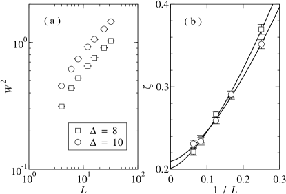
Figure 1: (a) $W$ vs. $L$ in a log-log plot at $\Delta=8$ and $10$ (strong disorder). (b) $\zeta$ vs. $1/L$ for the same values of $\Delta$ as in (a). The solid lines are least square fits to the form $\zeta(L)=\zeta+aL^{-b}$. We obtain $\zeta=0.21\pm 0.01$ and the resulting value of $b\simeq 1.5>1$ indicates that the extrapolation is stable against statistical uncertainties.

We first examine the power-law scaling behavior of the width, $W\sim L^{\zeta}$, in the rough phase at large disorder strength $\Delta=8$ and $10$. Figure 1 (a) shows the width average over $1000\sim 5000$ disorder realizations for $L=4\sim 32$. A noticeable curvature in the log-log plot indicates that corrections to scaling are still rather strong. Nevertheless, we can estimate the roughness exponent by extrapolating an effective exponent $\zeta(L)=\log[W(2L)/W(L)]/\log 2$ to the limit $L\rightarrow\infty$ by fitting it to a form $\zeta(L)=\zeta+aL^{-b}$, see Fig. 1 (b). We obtain that

$$\zeta=0.21\pm 0.01\ .$$ (5)

This value is consistent with the previous analytical and numerical results fisher86 ; halpin-healy90 ; middleton95 ; alava96 .

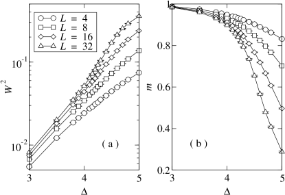
Figure 2: The interface width (a) and the order parameter (b) as functions of $\Delta$ at $L=4,8,16$, and $32$. They are obtained from the disorder average over $3000\sim 20000$ samples.

As the disorder strength decreases, the width also decreases and the interface eventually becomes flat below a threshold (see Fig. 2). The order parameter also shows an indication of a phase transition around $\Delta\simeq 4.0$. Apparently the order parameter decreases continuously. Therefore we perform a scaling analysis assuming that the phase transition is a continuous one. The critical point $\Delta_{c}$ can be determined from the finite-size-scaling property of the order parameter:

$$m(L,\varepsilon)=L^{-\beta/\nu}{\cal F}(\varepsilon L^{1/\nu})\ ,$$ (6)

where $\varepsilon\equiv\Delta-\Delta_{c}$, and $\beta$ ($\nu$) is the order parameter (correlation length) exponent. The scaling function ${\cal F}(x)$ has a limiting behavior ${\cal F}(x\rightarrow 0)=\mbox{const.}$ so that the order parameter decays algebraically with $L$ as $m\sim L^{-\beta/\nu}$ at the critical point. It also behaves as ${\cal F}(x\rightarrow-\infty)\sim|x|^{\beta}$ so that $m\sim|\varepsilon|^{\beta}$ for $\Delta<\Delta_{c}$ in the infinite system size limit.

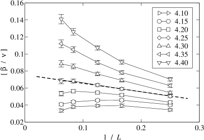
Figure 3: The effective exponent $[\beta/\nu](L)$ for different values of $\Delta$ as a function of $1/L$. The broken line is a guide for the eyes that separates the curves with a downward bending ($\Delta<\Delta_{c}$) from those with an upward bending ($\Delta>\Delta_{c}$).

Consider the effective exponent $[\beta/\nu](L)=-\log(m(2L)/m(L))/\log 2$. It converges to the value of $\beta/\nu$ at the critical point and deviates from it otherwise as $L$ increases. We estimate the critical threshold as the optimal value of $\Delta$ at which the effective exponent approaches a nontrivial value. The plot for this effective exponent is shown in Fig. 3. One can see that there is a downward and upward curvature for $\Delta<4.20$ and $\Delta>4.30$, respectively. From this behavior we estimate that $\Delta_{c}=4.25\pm 0.05$ and

$$\frac{\beta}{\nu}=0.07\pm 0.03\ .$$ (7)

Note that the effective exponent varies with $L$ even at the estimated critical point, which implies that corrections to scaling are not negligible for system sizes up to $L=32$. For that reason our numerical results for $\Delta_{c}$ and $\beta/\nu$ have rather large error bars, and one may need larger system sizes for better precision. The exponents $\beta$ and $\nu$ could also be obtained from the scaling analysis using Eq. (6). We fix the values of $\Delta_{c}$ and $\beta/\nu$ to the values obtained before and vary $\nu$ to have an optimal data collapse. We obtain

$$\nu=1.4\pm 0.2$$ (8)

and the corresponding scaling plot is shown in Fig. 4.

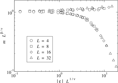
Figure 4: Scaling plot of $mL^{\beta/\nu}$ vs. $|\varepsilon|L^{1/\nu}$ with $\varepsilon=\Delta-4.25$, $\beta/\nu=0.07$, and $\nu=1.4$.

The order-parameter scaling property shows that the roughening phase transition is a continuous transition, though the exponent $\beta\simeq 0.1$ is very small, as opposed to the results of the GV study bouchaud92 predicting a first order transition. The transition nature becomes more transparent by looking at the probability distribution $P(m)$ of the magnetization near the critical point. We measured the distribution from a histogram of the magnetization of 3000 samples with $L=32$, which is shown in Fig. 5. We do not observe a double-peak structure in $P(m)$, which would appear for a first order transition, at any values of $\Delta$. Instead, there is a single peak which shifts continuously toward zero as $\Delta$ increases. We did not observe any double-peak structure in the distribution of the width, either. Therefore we conclude that the roughening transition is the continuous transition.

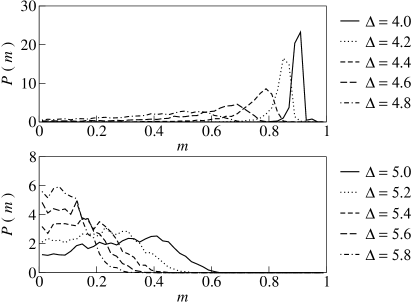
Figure 5: Histograms for the probability distribution $P(m)$ of the magnetization at $L=32$.

We note that this behavior is reminiscent of the three-dimensional random field Ising-model (RFIM) rfim , where also a very small order is found. This causes an extremely weak systems size dependence and the transition appears to be discontinuous in the order parameter although the system is indeed critical and the correlation length diverges. However, as has been pointed out in sourlas the magnetization of an individual sample shows close to the transition discontinuous jumps when (for a fixed field distribution) the coupling strength is varied (however, the sample-averaged magnetization is smooth). Since in the 3d RFIM the maximum jump does not vanish even in the infinite size limit some objection against the continuity of the phase transition has been raised sourlas . Since we find also a small order parameter exponent – and because of some model specific similarities between the 3d RFIM and the system we study here — we now want to check the jump size statistics, too.

For a given realization of $J$ and $V_{R}$ in Eq. (4), we measure the order parameter and its jumps when changing $V_{R}$ with a global factor. The interface may undergo two types of intermittence: The average height $\langle h\rangle$ may jump with a vanishing overlap of the interface configurations before and after the jump (meaning that the whole manifold is in a new position, uncorrelated with the previous one). Or a large domain type excitation may appear with only a small change in $\langle h\rangle$. The intermittent behavior of (1+1) and (2+1)D interfaces were studied in great detail in Ref. seppala01 . We want to study how the interface at a given average height roughens, therefore we only take into account the domain type excitations with the change in $\langle h\rangle$ less than one half when measuring the jump of the order parameter.

We calculate the order parameter in the interval $3\leq\Delta\leq 7$ with spacing 0.02. Figure 6 shows the probability distribution of maximum values of the jump $\delta m$ in $1000\sim 5000$ samples of sizes $L=4,6,8,12,16$. The inset shows the averaged value. It is non-zero, but becomes smaller as the system size increases except for the case of $L=4$. The decay is very slow, nevertheless we could fit the data for $L\geq 6$ to a form $\delta m\sim L^{-0.16}$ as can be seen in the inset. It suggests that the order parameter jump vanishes in the infinite size limit, and the smallness of the estimated exponent $0.16$ is compatible with our small estimate for the order parameter $\beta$.

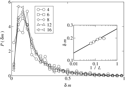
Figure 6: Order parameter jump distribution. Inset shows the plot of the averaged value vs. $1/L$ in the log-log scale. The solid line has a slope of 0.16.

We also studied the scaling of the width at the critical point. One might expect that the width at the critical point scales as $W\sim L^{\zeta^{\prime}}$ with a new roughness exponent $\zeta^{\prime}$ different from $\zeta\simeq 0.21$ for the rough interface. We plot the effective exponent $\zeta=\log[W(2L)/W(L)]/\log 2$ near the critical point in Fig. 7 (a). One observes that this effective exponent does not extrapolate to a non-zero value (for comparison c.f. Fig. 1 (b)). Instead, it decreases rapidly as $L$ grows, which suggests rather a logarithmic scaling, $W^{2}\simeq A\log L$, at the critical point as in the case of the periodic elastic medium noh01 . To investigate such a possibility, we measure the prefactor $A\equiv(W^{2}(2L)-W^{2}(L))/\log 2$ for this logarithmic scaling. They are also plotted in Fig. 7 (b), which shows a clear threshold behavior: It decreases (increases) for $\Delta<4.25$ ($>4.25$) and remains constant ($A\simeq 0.03$) at $\Delta=4.25$, which was estimated as the critical point from the order parameter scaling analysis. These facts are consistently suggesting that the interface width scales logarithmically at the critical point:

$$W^{2}\simeq 0.03\log L\ .$$ (9)

The result of the logarithmic scaling of the width at the critical point agrees well with that of the FRG study emig98 .

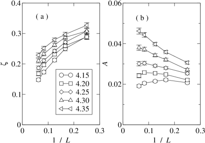
Figure 7: (a) Effective exponent for the power-law behavior of $W\sim L^{\zeta}$. (b) Prefactor in the logarithmic scaling of $W^{2}\simeq A\log L$.

Our numerical results pose an interesting question: In recent work noh01 we found that the disorder-driven roughening transition of the PEM appears to be independent of the commensurability parameter $p$ noh01 . As mentioned before, the elastic manifold can be seen as the $p\to\infty$ limit of the PEM. Based on this observation one might speculate that the roughening transitions of both systems belong to the same universality class. Although the $p\to\infty$-limit of the PEM could also belong to a different universality class the numerical results are compatible with the roughening transition in the EM and the PEM belonging to the same universality class:: For the EM we obtain $\beta/\nu\simeq 0.07$, $\nu\simeq 1.4$, and $A\simeq 0.03$ ($W^{2}\simeq A\log L$ at the critical point), while for the PEM noh01 we got $\beta/\nu\simeq 0.05$, $\nu\simeq 1.3$, and $A\simeq 0.018$. Although these values are very close to each other, a final conclusion could not be drawn yet due to the rather strong correction to finite size scaling observed in our study of the EM. So we have to leave this issue as an open question.

In summary, we have studied the $(3+1)$D elastic manifold in a crystal with quenched random impurities. We have investigated numerically the disorder-driven roughening transition at zero temperature using an exact combinatorial optimization algorithm technique. The transition turns out to be continuous with the critical exponents $\beta/\nu\simeq 0.07$ and $\nu\simeq 1.4$. For a given disorder potential configuration, the order parameter shows a discrete jump for finite size systems when varying its strength. However, the jump vanishes in the infinite system size limit. We also found that $W^{2}$ scales logarithmically with the system size $L$ at the critical point, in contrast to the power-law scaling in the rough phase. Our results do not agree with the scenario proposed in Ref. bouchaud92 that the roughening transition should be first order. Instead, they are in a qualitative agreement with those of FRG $\epsilon$-expansion study in Ref. emig98 , which predicts a continuous roughening transition and a logarithmic divergence of $W^{2}$ at the critical point. However, there is a significant discrepancy between the values of the critical exponents obtained numerically and analytically, which was also observed in the study of the PEM noh01 .

Acknowledgement: We thank J.P. Bouchaud for a stimulating discussion that motivated us to check the jump size statistics. This work has been supported financially by the Deutsche Forschungsgemeinschaft (DFG).

References

- (1) T. Halpin-Healy and Y.-C. Zhang, Phys. Rep. 254, 215 (1995).
- (2) J.-P. Bouchaud and A. Georges, Phys. Rev. Lett. 68, 3908 (1992).
- (3) T. Emig and T. Nattermann, Eur. J. Phys. B 8, 525 (1999).
- (4) A. I. Larkin, Sov. Phys. JETP 31, 784 (1970).
- (5) D. S. Fisher, Phys. Rev. Lett. 56, 1964 (1986).
- (6) T. Halpin-Healy, Phys. Rev. A 42, 711 (1990).
- (7) A. A. Middleton, Phys. Rev. E 52, R3337 (1995).
- (8) M. J. Alava and P. M. Duxbury, Phys. Rev. B 54, 14990 (1996).
- (9) E. T. Seppälä, M. J. Alava, and P. M. Duxbury, Phys. Rev. E 63, 036126 (2001).
- (10) T. Emig and T. Nattermann, Phys. Rev. Lett. 81, 1469 (1998).
- (11) T. Giamarchi and P. Le Doussal, Phys. Rev. Lett. 72, 1530 (1994); Phys. Rev. B 52, 1242 (1995).
- (12) D. McNamara and A. A. Middleton, and C. Zeng, Phys. Rev. B 60, 10062 (1999).
- (13) J. D. Noh and H. Rieger, Phys. Rev. Lett. 87, 176102 (2001).
- (14) T. Emig and T. Nattermann, Phys. Rev. Lett. 79, 5090 (1997).
- (15) M. Alava, , P. M. Duxbury, C. Moukarzel, and H. Rieger, in Phase Transitions and Critical Phenomena Vol. 18, (ed. C. Domb and J. L. Lebowitz), p. 141-317, (Academic Press, Cambridge, 2000); A. Hartmann and H. Rieger, Optimization Algorithms in Physics (Wiley VCH, Berlin, 2002).
- (16) A. K. Hartmann and U. Nowak, Eur. Phys. J. B 7, 105 (1999).
- (17) H. Rieger und A. P. Young, J. Phys. A 26, 5279, (1993); H. Rieger, Phys. Rev. B 52, 6659 (1995); A. A. Middleton and D. S. Fisher, Phys. Rev. B 65, 134411 (2002) and references therein.
- (18) J.-C. Anglès d’Auriac and N. Sourlas, Europhys. Lett., 39, 473 (1997).