Cluster persistence in one-dimensional diffusion–limited cluster–cluster aggregation

Abstract

The persistence probability, $P_{C}(t)$, of a cluster to remain unaggregated is studied in cluster-cluster aggregation, when the diffusion coefficient of a cluster depends on its size $s$ as $D(s)\sim s^{\gamma}$. In the mean-field the problem maps to the survival of three annihilating random walkers with time-dependent noise correlations. For $\gamma\geq 0$ the motion of persistent clusters becomes asymptotically irrelevant and the mean-field theory provides a correct description. For $\gamma<0$ the spatial fluctuations remain relevant and the persistence probability is overestimated by the random walk theory. The decay of persistence determines the small size tail of the cluster size distribution. For $0<\gamma<2$ the distribution is flat and, surprisingly, independent of $\gamma$.

I Introduction

Aggregation models are useful in describing various phenomena from chemical engineering, material sciences, atmosphere research to even astrophysics Meakin:PhysicaScripta46 ; Friedlander_book ; Family_Landau . One general property of these models is that they lead to dynamic scale-invariance: when all the lengths are scaled by the characteristic length, the system looks the same at different times. Lately, studies of first passage problems rednerinkirja under the name persistence Majumdar:CurrSciIndia ; Majumdar:PRL77 ; Derrida:PRL77 have shown that not necessarily all the properties of a dynamically scaling system are characterized by a single scale Bray:PRE62 . Here we address the probability of a cluster to remain intact in an aggregation system and show how this quantity and the associated length scale relate to the physically relevant issue of the shape of the cluster size distribution.

In an aggregation system one can define many first-passage problems and related quantities omapers . We study the probability that a cluster has not aggregated with any other one before time $t$ Hellen:EPL . This probability is called cluster persistence and denoted by $P_{C}(t)$. Similar problems considering uninfected walkers in one-dimensional reaction-diffusion systems ODonoghue:CM1 and Potts model ODonoghue:CM2 have recently been shown to display interesting behavior. We concentrate on diffusion–limited cluster–cluster aggregation (DLCA) in one dimension, where the dynamics is dominated by spatial fluctuations Kang:PRA30 . For high dimensional systems these may be neglected, and on the mean-field level, valid for dimensions higher than the upper critical dimension, aggregation is well understood vanDongen:PRL54 ; vanDongen:JSP50 ; vanDongen:PRL63 .

The DLCA model is defined so that the nearest neighbor occupied sites in a lattice are identified as a cluster. Each cluster diffuses with a size dependent diffusion constant, $D(s)\sim s^{\gamma}$, where $\gamma$ is the diffusion exponent. If a cluster collides with another one, the two clusters are irreversibly merged together and the aggregate diffuses either faster ($\gamma>0$) or slower ($\gamma<0$) than either of the colliding clusters. While the size independent diffusion ($\gamma=0$) is exactly solvable in one dimension, it forms a marginal case between two completely different aggregation mechanisms Hellen:PRE62 . We study here the more physically interesting problem with $\gamma\neq 0$.

The aim is to study the dependence of cluster persistence on the diffusion exponent $\gamma$ and extend the study presented in Ref. Hellen:EPL . We also pay attention to the random-walk (RW) problems that ensue as on a mean-field level the problem is reduced to the survival of three annihilating random walkers. While the $\gamma=0$ case is readily solvable by various methods Fisher:JSP34 ; Derrida:PRE54 , already the case of three annihilating particles with unequal diffusion constants is rather involved Fisher:JSP53 . Here $\gamma\neq 0$ leads to time dependent diffusion coefficients, and we derive a Fokker-Planck (FP) equation for the survival of these particles. For $\gamma\geq 0$ its analysis yields an algebraically decaying survival probability, $P_{\rm surv}(t)\sim t^{-\theta_{\rm RW}(\gamma)}$. The survival exponent $\theta_{\rm RW}$ is discontinuous and non-monotonic as it is given by $\theta_{\rm RW}(\gamma)=2/(2-\gamma)$ for $0<\gamma<2$ and $\theta_{\rm RW}(0)=3/2$. The numerical comparison of the survival and persistence probabilities validates the theory and hence $P_{C}(t)\sim t^{-\theta_{C}}$ with $\theta_{C}=\theta_{\rm RW}$.

For $\gamma<0$ simulations show that both the survival and persistence probabilities decay stretched exponentially as $\exp(-Ct^{\beta})$. The Fokker-Planck equation is not amenable to analytic analysis, so we use a Lifshitz tail argument to understand the survival. Such heuristic arguments and numerics suggest a stretching exponent $\beta_{\rm RW}(\gamma)=-\gamma/(4-2\gamma)$. The Lifshitz tail argument indicates that the exponent is affected by the fluctuations in the motion of the particles that neighbor the surviving one. These are taken into account only approximately in the mean-field theory and for the DLCA numerics gives $\beta_{C}=-2\gamma/(6-3\gamma)$. A closer examination reveals that also the distance distribution between the particles surrounding a surviving one in the mean-field model scales in a different way than the corresponding distribution of the DLCA.

In addition, we show how the cluster persistence is related to the cluster size distribution. To clarify the connection, consider the dynamic scaling in DLCA. Both simulations and experiments show that the cluster size distribution $n_{s}(t)$ (the number of cluster of size $s$ per lattice site at time $t$) scales as Meakin:PhysicaScripta46

$$n_{s}(t)=S(t)^{-2}f\left(\frac{s}{S(t)}\right),$$ (1)

where $S(t)\sim t^{z}$ is the average cluster size and the scaling limit, $s\to\infty$ and $S(t)\to\infty$ with $s/S(t)$ fixed, is taken. In one dimension the dynamic exponent $z=1/(2-\gamma)$ Miyazima:PRA36 ; Kang:PRA33 . For $\gamma\geq 0$ the cluster size distribution is broad in the sense that the scaling function behaves as $f(x)\sim x^{-\tau}$ as $x\equiv s/S(t)\to 0$. For $\gamma<0$ the scaling function is bell-shaped and $f(x)\sim\exp(-Ax^{-|\mu|})$ for $x\to 0$, where $A$ is a constant. To determine the polydispersity exponent, $\tau$, which characterizes the number of small clusters, is non-trivial even on a mean-field level vanDongen:PRL54 ; Cueille:PRE55 whereas the similar exponent $\mu$ readily follows from scaling analysis vanDongen:JSP50 . All the exponents $z$, $\tau$, and $\mu$ are universal, i.e., they do not depend on the fine details of the model. They can, and it is natural to expect that they do, depend on the diffusion exponent $\gamma$.

One of the main results of this paper is that the exponents describing the decay of the cluster persistence are related to these universal exponents as

$$\theta_{C} = (2-\tau)z$$ (2a)

$$\beta_{C} = |\mu|z.$$ (2b)

Quite unexpectedly, the polydispersity exponent is a constant, $\tau=0$, for $0<\gamma<2$, but discontinuous since $\tau(\gamma=0)=-1$. The reasoning leading to the relations (2a) and (2b) is universally applicable, so that the behavior of the tail of cluster size distribution might be tackled through cluster persistence in other models, too.

The outline of the paper is as follows. In section II the mean-field random walk theory is formulated and the associated Fokker-Planck equation is derived. Section III starts by describing the simulation methods. Thereafter the mean-field theory is validated for $\gamma\geq 0$ by comparing the survival probability obtained from the analysis of the Fokker-Planck equation to the simulation results of both the random walk system and the DLCA one. For $\gamma<0$ a similar comparison shows the effect of spatial fluctuations, and the stretched exponential decay of the survival probability is explained using a Lifshitz tail argument. Section IV concentrates on the relation between the persistence and the small size tail of the cluster size distribution. The paper ends with conclusions in section V.

II Mean-Field: Reduction to a Three Particle Problem

The two clusters surrounding a persistent one will grow when they collide with other clusters (but not with the persistent one). The cluster in the middle will be persistent until it collides with one of the neighbors. After this the two remaining clusters would contribute to persistence only by increasing the mass of the clusters surrounding another persistent cluster. This is negligible at late times, since the persistent clusters will be separated by many non-persistent ones, i.e. $t^{\theta_{C}}\gg t^{z}$. In other words, the correlations in the system grow only as $t^{z}$ and each persistent cluster is asymptotically independent. Thus it is sufficient to consider only one persistent cluster and its two neighbors.

The collisions of the surrounding clusters make them bigger and increase or decrease the diffusivity. We make the mean-field approximation that each cluster neighboring a persistent one will grow as an average cluster does. Hence, we replace the true process, where the surrounding clusters collide at some discrete times $t_{i}$, by a continuous one, where the surrounding clusters grow as $S(t)$. As $D(s)\sim s^{\gamma}$ these clusters will diffuse with time-dependent diffusion coefficients. In the following analysis we will ignore the possible early time crossover effects in the growth of the average cluster size and the diffusion coefficients of the clusters surrounding a persistent one are taken to follow a true power-law at all times. This will only affect the early time behavior.

The finite extent of clusters is irrelevant for cluster persistence and we will consider the three clusters as point-like particles from now on. Let $x_{i}(t)$ ($i=1,2,3$) denote the positions of the particles at time $t$ such that $x_{1}(0)<x_{2}(0)<x_{3}(0)$. The motion of these is described by the Langevin equations

$$\dot{x}_{i}(t)=\xi_{i}(t),$$ (3)

with Gaussian white noises $\langle\xi_{i}(t)\rangle=0$ and $\langle\xi_{i}(t)\xi_{j}(t^{\prime})\rangle=2{\cal D}_{i}(t)\delta_{ij}\delta(t-t^{\prime})$. The overdot denotes derivative with respect to time and the brackets an ensemble average over different realizations. The diffusion coefficients of the particles read as ${\cal D}_{1}(t)={\cal D}_{3}(t)=D_{1}t^{\gamma z}$ and ${\cal D}_{2}(t)=D_{2}$. The meaning of a time-dependent diffusion coefficient, say ${\cal D}_{1}(t)$, is simply that the particle $1$ will follow a simple diffusive motion with a diffusion constant $D_{1}$ in the time scale

$$T_{1}(t)=\int_{0}^{t}{\rm d}t^{\prime}{\cal D}_{1}(t^{\prime})/D_{1}=t^{\gamma z+1}/(\gamma z+1).$$ (4)

As we are interested in the survival of the middle particle ($x_{2}$), the process terminates when either $x_{1}=x_{2}$ or $x_{2}=x_{3}$. It is convenient to consider the distances between the particles: $x_{12}(t)=x_{2}(t)-x_{1}(t)\geq 0$ and $x_{23}(t)=x_{3}(t)-x_{2}(t)\geq 0$. These obey similar Langevin equations

$$\begin{cases}{\dot{x}}_{12}(t)=\Gamma_{12}(t)\\ {\dot{x}}_{23}(t)=\Gamma_{23}(t),\end{cases}$$ (5)

where $\langle\Gamma_{12}(t)\rangle=\langle\Gamma_{23}(t)\rangle=0$ and $\langle\Gamma_{12}(t)\Gamma_{12}(t^{\prime})\rangle=\langle\Gamma_{23}(t)\Gamma_{23}(t^{\prime})\rangle=2(D_{2}+D_{1}t^{\gamma z})\delta(t-t^{\prime})$. The two noises are correlated as the motion of the middle particle affects both distances: $\langle\Gamma_{12}(t)\Gamma_{23}(t^{\prime})\rangle=-\langle\xi_{2}(t)\xi_{2}(t^{\prime})\rangle=-2D_{2}\delta(t-t^{\prime})\neq 0$. For $\gamma>0$ the noise correlations become asymptotically irrelevant, which is not the case for $\gamma<0$.

To proceed, we transform Eqs. (5) to a Fokker-Planck equation for the probability density $\rho(x_{12},x_{23};t)$ of the two distances at time $t$. Due to the mutual correlations this is easiest to do by computing the drift and diffusion coefficients from their definitions

$$D_{i} =\lim_{\Delta t\to 0}\frac{1}{\Delta t}\left\langle x_{i}(t+\Delta t)-x_{i}(t)\right\rangle$$

$$D_{ij} =\frac{1}{2}\lim_{\Delta t\to 0}\frac{1}{\Delta t}\langle[x_{i}(t+\Delta t)-x_{i}(t)][x_{j}(t+\Delta t)-x_{j}(t)]\rangle$$

and insert these to the general Fokker-Planck equation Risken:book

$${{\partial\rho}\over{\partial t}}=-\sum_{i=1}^{2}{{\partial}\over{\partial x_{i}}}D_{i}\rho+\sum_{i,j=1}^{2}{{\partial^{2}}\over{\partial x_{i}\partial x_{j}}}D_{ij}\rho.$$ (6)

A straightforward calculation gives

$$\frac{\partial{\rho}}{\partial t}=(D_{2}+D_{1}t^{\gamma z})\left(\frac{\partial^{2}{\rho}}{\partial x_{12}^{2}}+\frac{\partial^{2}{\rho}}{\partial x_{23}^{2}}\right)-2D_{2}\frac{\partial^{2}{\rho}}{\partial x_{12}\partial x_{23}}.$$ (7)

The initial condition is now $\rho(x_{12},x_{23};0)=\delta(x_{12}-x_{12}^{0})\delta(x_{23}-x_{23}^{0})$, where $x_{12}^{0}=x_{12}(0)$ and $x_{23}^{0}=x_{23}(0)$ are the initial distances between particles. The termination of the process when two particles collide gives absorbing boundary conditions along the axis, i.e., $\rho(x_{12},0;t)=0$ and $\rho(0,x_{23};t)=0$ for all times $t$.

Thus the original many body problem has been reduced to the survival of three annihilating random walkers. Given that one can solve Eq. (7) with the appropriate boundary conditions, the survival probability of the middle particle (which corresponds to the persistent cluster) can be obtained as

$$P_{\rm surv}(t)=\int_{0}^{\infty}{\rm d}x_{12}\int_{0}^{\infty}{\rm d}x_{23}\ \rho(x_{12},x_{23};t).$$ (8)

When the survival probability decays algebraically, $P_{\rm surv}(t)\sim t^{-\theta_{\rm RW}}$, the associated exponent $\theta_{\rm RW}$ is called the survival exponent.

III Comparison of the Simulations and Theory

III.1 Details of Simulations

The DLCA simulations are done on a lattice of size $L$ with periodic boundary conditions. Concentration $\phi$ of sites is filled with particles and nearest neighbor particles belong to the same cluster. The initial distribution is either monodisperse, $n_{s}(0)=\delta_{1,s}$, with equal distances, $l_{0}$, between neighboring clusters or random, in which case each site is independently filled with probability $\phi$. The persistence exponent is independent of the initial distribution but the early time behavior of the persistence probability depends on it omapers .

In the dynamical evolution a cluster is selected randomly and time is increased by $1/[N(t)D_{\rm max}(t)]$. Here $N(t)$ denotes the number of clusters and $D_{\rm max}(t)$ is the maximum of the diffusion coefficients of all the clusters at time $t$. The cluster is moved one lattice spacing with cluster size dependent probability $D(s)/D_{\rm max}(t)$. If the cluster collides with another one, the clusters are irreversibly aggregated together and the values of $N$ and $D_{\rm max}$ are updated. Then a new cluster is selected and the above procedure is repeated.

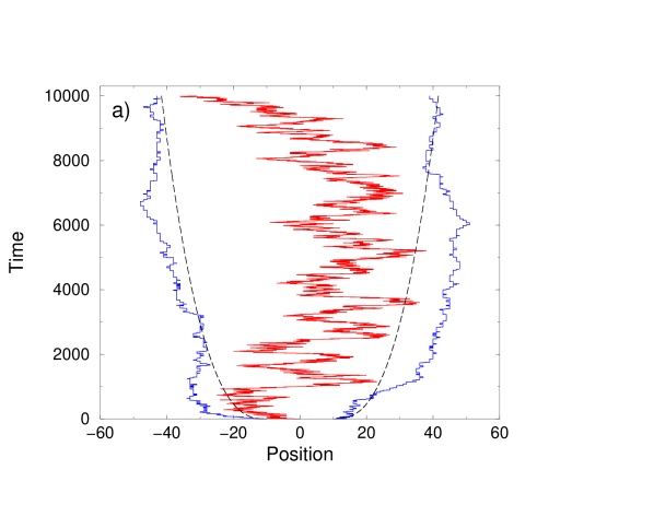
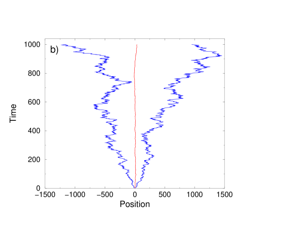
Figure 1: Visualization of the three particle system when the initial distance $l_{0}=10$ for a) $\gamma=-2$ ($z=1/4$) and b) $\gamma=1$ ($z=1$). The probabilities of these configurations are of order $10^{-8}$ and $10^{-4}$, respectively. At the final time the ratio $D_{2}/(D_{1}t^{\gamma z})$ is about $10^{2}$ in (a) and $10^{-3}$ in (b). The dashed lines in (a) show $t^{\alpha}$-behavior with $\alpha=0.375$ (see Section III.4 for details).

The three particle simulation is similar to that of the DLCA. Initially the distance between particles is $l_{0}$. A particle $i\in\{1,2,3\}$ is selected randomly and it is moved a distance $a$ either to the left or to the right with probability ${\cal D}_{i}(t)/{\cal D}_{>}(t)$. Here ${\cal D}_{>}(t)={\rm max}\{{\cal D}_{1}(t),D_{2},{\cal D}_{3}(t)\}$ is the maximum of the diffusion coefficients of the three particles at that time. The distance $a$ is set to correspond the lattice constant of the DLCA simulations, i.e., $a=1$. Irrespective of the movement of the particle time is increased by $1/[3{\cal D}_{>}(t)]$ and the time-dependent diffusion coefficients ${\cal D}_{1}(t)$ and ${\cal D}_{2}(t)$ are updated to new values. This procedure continues until a collision occurs. Figure 1 shows examples of configurations that survive for a long while for negative and positive values of the diffusion exponent.

The faster the survival probability decays the more computation time is used in simulating systems, which terminate at early times. In order to sample efficiently the long living, interesting configurations we use a cloning method Grassberger1 ; Grassberger2 for the three particle simulations when $\gamma<0$: At times $t_{j}$ we make $n_{j}$ copies of all the systems, which have survived upto this time. Typically simulations are averaged over $5\times 10^{6}$ initializations and the system is copied at times $10$, $10^{2}$, and $10^{3}$ with $2\times 10^{3}$, $5\times 10^{4}$, and $10^{4}$ copies, respectively. This enables us to reach probabilities less than $10^{-15}$.

III.2 Size-Independent Diffusion ($\gamma=0$) and Crossover Behavior

When the diffusion constant of a cluster does not depend on its size, i.e.  $\gamma=0$, an exact solution is possible as the collisions of the clusters surrounding a persistent one with other clusters do not matter Spouge:PRL60 . For the same reason the mean-field approximation becomes exact and reduces to an old problem of the survival probability of three similar annihilating random walkers Fisher:JSP34 . The persistence and survival exponents attain the value $3/2$.

This result can also be obtained from the equation (7) which for this particular case simplifies to

$$\frac{\partial{\rho}}{\partial t}=(\frac{\partial^{2}{\rho}}{\partial x_{12}^{2}}+\frac{\partial^{2}{\rho}}{\partial x_{23}^{2}})-\frac{\partial^{2}{\rho}}{\partial x_{12}\partial x_{23}},$$ (9)

where we have taken $D_{1}=D_{2}=1/2$. A coordinate transformation $x=(x_{12}+x_{23}),y=(x_{12}-x_{23})/\sqrt{3}$ reduces this to a diffusion equation

$$\frac{\partial{\rho}}{\partial t}=\frac{\partial^{2}{\rho}}{\partial x^{2}}+\frac{\partial^{2}{\rho}}{\partial y^{2}}$$ (10)

with the boundary condition $\rho=0$ along lines $y=\pm x/\sqrt{3}$. This corresponds to a two-dimensional wedge of angle $\Theta=\pi/3$, in which the survival probability decays as $t^{-\pi/2\Theta}\sim t^{-3/2}$ rednerinkirja .

It is also interesting to know how the asymptotic regime, where $P_{\rm surv}(t)\sim t^{-\theta_{\rm RW}}$, is reached. In the case $D_{1}=D_{2}=D_{3}=D$ ($\gamma=0$) with the initial distances between particles being $x_{12}^{0}=x_{23}^{0}=l_{0}$ the solution including the first correction to scaling is given by Derrida:PRE54 ; Spouge:PRL60

$$P_{\rm surv}(t)\approx\frac{1}{4\sqrt{2\pi}}\left(\frac{l_{0}^{2}}{Dt}\right)^{3/2}\left(1-\frac{3}{16}\frac{l_{0}^{2}}{Dt}\right).$$ (11)

The correction becomes negligible for times much larger than the crossover time $t_{\rm cr}=3l_{0}^{2}/(16D)$. For $\gamma\neq 0$ the corrections go in powers of the ratio of the diffusion coefficients, $D_{2}/D_{1}t^{\gamma z}$. For $\gamma>0$ this is demonstrated in Appendix A and for the corresponding two particle problem it may be shown exactly (see Appendix B). Therefore the crossover time depends on $\gamma$ as $t_{\rm cr}\sim r^{(2-\gamma)/|\gamma|}$, where the constant $r\approx 30$ according to simulations. As $t_{\rm cr}$ diverges for $|\gamma|\to 0$, we can expect that the asymptotic scaling regime can be reached in simulations only for relatively large values of $|\gamma|$.

III.3 Validation of the Mean-Field Theory ($\gamma>0$)

We have not been able to solve equation (7) exactly. The reason is that the absorbing boundary conditions together with the two time scales appearing in the problem make the standard methods (Laplace or Fourier transforms; polar coordinates) unapplicable. Nor is it possible to transform the equation to a diffusion equation with simple enough boundary conditions. However, the full solution is not needed for the determination of the survival exponent since this is given by the leading large time behavior when $t\to\infty$. It would only provide us information about the crossover effects, which according to our analysis (see Appendix A) and the numerical simulations (see below) are rather pronounced when $\gamma$ is close to zero.

A change of variables $x=(x_{12}+x_{23})/\sqrt{2},y=(x_{12}-x_{23})/\sqrt{2}$ transforms Eq. (7) to

$$\frac{\partial{\rho}}{\partial t}=D_{1}t^{\gamma z}\frac{\partial^{2}{\rho}}{\partial x^{2}}+(D_{1}t^{\gamma z}+2D_{2})\frac{\partial^{2}{\rho}}{\partial y^{2}}$$ (12)

with the boundary condition $\rho=0$ along $y=\pm x$, i.e., a wedge of angle $\Theta=\pi/2$. When $\gamma>0$ the constant term is negligible at long times ($D_{1}t^{\gamma z}\gg D_{2}$) and the diffusion becomes isotropic. This can be shown by directly solving equation (7) and analyzing the large time behavior of the solution (Appendix A). A change to the time scale $T_{1}$ [see Eq. (4)] transforms Eq. (12) to the form of Eq. (10) and the survival probability $P_{\rm surv}(t)\sim T_{1}^{-\pi/2\Theta}\sim T_{1}^{-1}\sim t^{-(1+\gamma z)}$. As $z=1/(2-\gamma)$ the survival exponent $\theta_{\rm RW}(\gamma)=2/(2-\gamma)=2z$.

The approximation of neglecting the constant term in Eq. (7) corresponds to a complete separation of the time scales, i.e., to a situation, where the middle particle is at rest ($D_{2}=0$). Thus for $\gamma>0$ one could simply determine the survival exponent by considering two independent random walkers with a fixed absorbing boundary in between [compare to Fig. 1 (b)]. In other words, the motion of the “slow” particle becomes asymptotically irrelevant. This can be exactly shown for the the corresponding two particle problem (Appendix B).

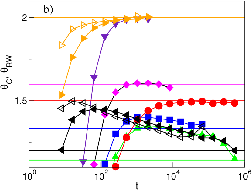
Figure 2: a) Comparison between the survival (filled symbols) and persistence (open symbols) probabilities. b) The corresponding local exponents. The horizontal lines correspond to the analytic values given by $\theta=2/(2-\gamma)$. The data for RW survival are averaged over variable number of realizations ranging from $10^{9}$ for $\gamma=0$ to $2\times 10^{7}$ for $\gamma=0.5$. The DLCA simulations are averaged over 50000 simulations on a system of size 55555. The initial distance between particles is $10$ (upper curves in Fig. a) or $2$ (lower curves).

Figure 2 compares the survival and persistence probabilities. The initial distances between particles in the random walk simulations are set to be the same as in the DLCA. The probabilities decay algebraically at large times and the only difference in the decay is between the amplitudes. This is to be expected as the transient effects of the growth of the average cluster size are not taken into account in the random walk picture.

The inset shows local exponents, i.e. logarithmic derivatives of the probabilities, which converge to the value obtained from the Fokker-Planck equation, $\theta_{\rm RW}=2/(2-\gamma)$ for $\gamma>0$ and $\theta_{\rm RW}=3/2$ for $\gamma=0$. The asymptotic regime is reached only for $\gamma=0$ and $\gamma\gtrsim 0.5$. In the latter region the local exponents saturate, when the ratio of the diffusion coefficients is of about $30$. For example, for $\gamma=0.25$ this would corresponds to $t_{\rm cr}\approx 2\times 10^{10}$ which is beyond the time reached in simulations.

Note that the persistence exponent is discontinuous and nonmonotonic at $\gamma=0$, i.e., $3/2=\theta_{C}(0)>\theta_{C}(0^{+})=1$. This seems first counterintuitive since making some of the clusters to diffuse faster helps others to survive longer! On the other hand, as time elapses a persistent cluster becomes slower as compared to an average one. In this way it eventually adopts the optimal strategy Redner:AJP67 by becoming stationary.

III.4 Fluctuation dominated persistence ($\gamma<0$)

For $\gamma<0$ the diffusion of the clusters surrounding a persistent one slows down. Consider the random walk picture and proceeding similarly as for $\gamma>0$ above. Fixing now particles $1$ and $3$ would lead to an interval of fixed length and hence to an exponentially decaying survival probability. However, simulations show that the survival decays stretched exponentially in time, $P_{\rm surv}(t)\sim\exp(-C_{\rm RW}t^{\beta_{\rm RW}})$. Furthermore, as will be shown below, although the surrounding particles become slower, their motion can not be neglected even at the long time limit. This is a collective effect and in clear contrast to the exactly solvable two particle case, where the fast particle eventually dominates the survival (Appendix B).

Figure 3: Survival probabilities for $\gamma=-2$ with $l_{0}=2$ (dashed), $3$ (dotted), and $4$ (dot-dashed). The solid line is a guide to eye with a slope $\beta_{\rm RW}=0.25$. The inset shows how the local stretching exponents converge to the same value independent of the initial distance $l_{0}$.

In figure 3 we plot $-\ln(P_{\rm surv}(t))$ vs. $t$ on a log-log scale so that a stretched exponential decay corresponds to a straight line with a slope $\beta_{\rm RW}$. The final slope is independent of the initial distance between particles, and thus the stretching exponent is universal.

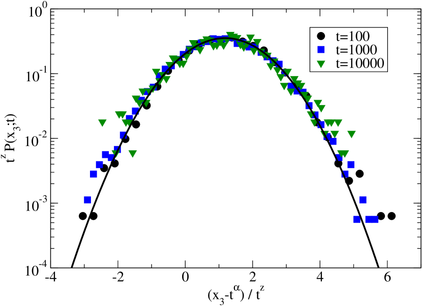
Figure 4: The scaling plot of the location distribution of the rightmost particle in the random walk simulations for $\gamma=-2$. The values of the scaling exponents are $z=1/4$ and $\alpha=3/8$. The solid line shows a Gaussian fit to the data.

Figure 4 shows the location distribution $p(x_{3};t)$ of the particle 3 (the one for the particle 1 would be the same). It scales as

$$p(x_{3};t)=t^{-z}g\left(\frac{x-bt^{\alpha}}{t^{z}}\right)$$ (13)

implying that although the distribution widens as $t^{z}$, the expectation value of the distance from the origin grows as $bt^{\alpha}$ with a non-trivial exponent $z<\alpha<1/2$ [see Fig. 1 (a)]. The scaling is similar to the reaction front in the originally separated reaction-diffusion system $A+B\to C$, where the reaction zone becomes sharp at late times, i.e. $z<\alpha$ Galfi:PRA88 ; Koza:PHYSA240 . It is striking that the scaling function $g(y)$ is within the numerical accuracy a simple Gaussian.

The consequence of Eq. (13) is that the average distance between the particles 1 and 3 grows [see Fig. 1 (a)]. If it would grow deterministically as $t^{\alpha}$, with $\alpha<1/2$, the survival probability would decay asymptotically stretched exponentially with the exponent $\beta_{\rm det}=1-2\alpha$ Krapivsky:AJP64 . For example, for $\gamma=-2.0$ the numerics gives a rough estimate $\alpha\approx 0.36$ and $1-2\alpha\approx 0.28$, which is in reasonable agreement with the numerically obtained stretching esponent $\beta_{\rm RW}\approx 0.25$ (see inset of Fig. 3).

To understand the origin of the new length scale $t^{\alpha}$ the next logical step is to try to take the length fluctuations of the interval into account. We make this using a Lifshitz tail approach rednerinkirja . It is based on the assumption that the main contribution to the survival is provided by extreme configurations, where the particles surrounding the surviving one have diffused far apart from each other. We write the survival probability as

$$P_{\rm surv}(t)\approx\int_{0}^{\infty}{\rm d}l\ P(l;t)Q(t|l),$$ (14)

where $P(l;t)$ is the probability distribution of the interval lengths $l=x_{3}-x_{1}$ around a surviving particle at time $t$ and $Q(t|l)\sim l^{-1}\exp(-\pi^{2}Dt/l^{2})$ is the survival probability of a particle in an interval of length $l$ rednerinkirja ; Weiss:book . In order to make progress, we need to know the large $l$ behavior of $P(l;t)$. It scales similarly as $p(x_{3};t)$

$$P(l;t)=t^{-z}G\left(\frac{l-2bt^{\alpha}}{t^{z}}\right),$$ (15)

where the large $y$ tail of $G(y)$ is Gaussian as the position distributions of particles 1 and 3 are Gaussian. Although it is irrelevant in what follows, the small $y$ part of $G(y)$ decays faster than the large $y$ tail due to the restriction $x_{3}>x_{1}$.

Denote the variance of the Gaussian tail of $G(y)$ by $\sigma^{2}$. Then Eq. (14) gives

$$P_{\rm surv}(t)\sim t^{z-\alpha}\int_{0}^{\infty}{\rm d}l\exp{\left(-\frac{(l-2bt^{\alpha})^{2}}{2\sigma^{2}t^{2z}}-\frac{\pi^{2}Dt}{l^{2}}\right)}.$$

When $t\to\infty$ the integrand becomes sharply peaked and may be evaluated using the saddle point method. This gives $\alpha=(2z+1)/4$ and

$$P_{\rm surv}(t)\sim t^{(6z-1)/4}e^{-Ct^{(1-2z)/2}}.$$ (16)

Inserting the value of $\alpha$ coming from the Lifshitz argument to the result of an algebraically expanding interval, $\beta_{\rm det}=1-2\alpha$, leads to the same streching exponent $\beta=(1-2z)/2$. These two results coincide, as a consequence of the peculiar scaling [Eq. (15)] and that the tail of the interval length distribution decays as $G(y)\sim\exp(-y^{2})$. We emphasize that the fluctuations of the surrounding, slow particles determine the stretching exponent and that it is purely a coincidence that the Lifshitz tail argument gives the same result as the use of the average value.

The stretching exponent $\beta_{\rm RW}=(1-2z)/2$ has an obvious interpretation. There are two length scales in the problem. The first one is related to the random walkers with time-dependent diffusion coefficients, $L_{1}\sim t^{z}$, and the other to the surviving particle, $L_{2}\sim t^{1/2}$. The argument of the exponential decay is simply the ratio of these two scales in the problem, $P_{\rm surv}(t)\sim\exp(-L_{2}/L_{1})$. Although reasonable, the calculation above shows the delicacy of the survival: the distance between the particles 1 and 3 involves a third, non-trivial length scale, $L_{3}\sim t^{\alpha}$, with $\alpha=(2z+1)/4$. The above considerations can also be made by resorting to an argument which considers the two characteristic time scales $T_{1}\sim t^{1+\gamma z}$ and $T_{2}\sim t$. It is easy to see, that the ratios between the scales obey a diffusive like scaling relation $L_{2}/L_{1}\sim\sqrt{T_{2}/T_{1}}$ such that any quantity involving the ratio of length scales may be given in terms of the ratio of the time scales and vice versa.

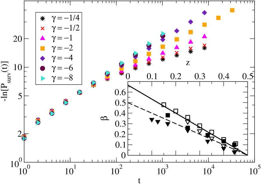
Figure 5: The survival probability for $\gamma<0$. The inset shows the bounds for the stretching exponents for the survival (filled symbols) and persistence (open symbols). For details see text. The dashed [solid] line is given by $(1-2z)/2$ [$2(1-2z)/3$].

In figure 5 the survival probabilities are plotted for $\gamma<0$ (for a similar figure for the persistence see figure 3 in Hellen:EPL ). In spite of being able to simulate rather small probabilities the asymptotic regime is not reached in the simulations. Similar problems with a slow convergence to the asymptotic value have been encountered in other reaction-diffusion systems Mehra:preprints ; Bray:preprint and they might be overcome by a more efficient use of the cloning method Grassberger1 ; Grassberger2 . The inset of Fig. 5 shows bounds for the stretching exponents as a function of the dynamic exponent $z=1/(2-\gamma)$. The upper bounds are obtained by fitting a line to the three or four largest time points and measuring the slope. To obtain the lower bound, we considered the change of the local slope and extrapolated to $1/t\to 0$, when it was possible. This method neglects the saturation of the local exponent after a finite crossover time and therefore gives a lower bound. For comparison, the corresponding bounds for persistence are also shown in the inset. There is a clear difference between the two. The numerics is consistent with the prediction $\beta_{\rm RW}=(1-2z)/2$, and for the persistence the data suggest an expression $\beta_{C}=2(1-2z)/3$.

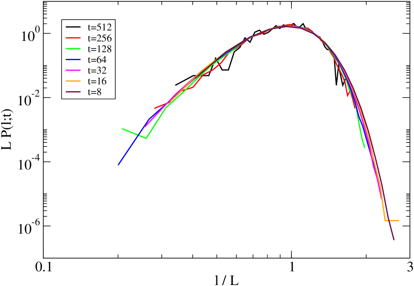
Figure 6: The scaling of the distance distribution between the clusters surrounding a persistent one in DLCA for $\gamma=-0.8$.

The difference between the mean-field model and the DLCA is further elucidated in figure 6. It shows that in the DLCA the distance distribution between the clusters surrounding a persistent one scales similar to that of the cluster size distribution

$$P(l;t)=L^{-1}h\left(\frac{l}{L}\right).$$ (17)

Hence, the distribution widens at the same rate as the average distance $L(t)\sim t^{z}$ grows in contrast to the RW case. For large $x$ the scaling function $h(x)\sim\exp(-bx)$ and the Lifshitz tail argument leads to an estimate $\beta_{\rm L}=(1-2z)/3$, which disagrees with the numerics.

The inconsistency is not surprising since in the DLCA there are fluctuations coming from the statistical nature of collisions, which are not taken into account in the Lifshitz approach. More precisely, the diffusion constants of the neighbors of persistent clusters have some unknown distribution. Furthermore, the diffusion constant also correlates with the distance from the persistent cluster. These facts together with the fact that the stretching exponent is determined by the fluctuations makes an analytical estimation of the persistence for $\gamma<0$ hard.

IV Implications for the Cluster Size Distribution

We now turn to the relation of the persistence to the cluster size distribution. We concentrate first on the case $\gamma>0$, when the cluster size distribution has a power-law tail at small cluster sizes. The dynamical scaling together with the definition of the dynamical and polydispersity exponents, $z$ and $\tau$, respectively, were discussed in the Introduction [Eq. (1)]. The scaling theory further states that all the cluster number densities decay in a similar manner at large times, i.e., $n_{s}(t)/n_{1}(t)\to b_{s}$ as $t\to\infty$ vanDongen:JPA18 , where $b_{s}$ is a constant. Here the exponent of interest is the universal decay exponent, $w$, which describes the decrease $n_{s}(t)\sim t^{-w}$.

Using $S(t)\sim t^{z}$ together with $f(x)\sim x^{-\tau}$ as $x\to 0$ in equation (1) gives $n_{s}(t)\sim t^{-(2-\tau)z}s^{-\tau}$ so that the three exponents defined above are related by the scaling relation $w=(2-\tau)z$ Vicsek:PRL52 . Therefore the full characterization of the dynamic scaling requires the knowledge of only two of the exponents. However, even on the mean-field level of Smoluchowski’s rate equation theory the only readily calculable exponent for DLCA is the dynamic exponent $z$. The difficulty with, for example, the polydispersity exponent $\tau$ arises from the fact that to calculate it requires the knowledge of the whole scaling function vanDongen:PRL54 . Next we argue how knowing the persistence exponent $\theta_{C}$ helps to overcome this problem.

Let us start from the trivial size independent case, $\gamma=0$, for which an exact solution of the cluster size distribution $n_{s}(t)$ is possible Spouge:PRL60 . The actual form of this distribution is not important for our purposes. The point is that the decay exponent $w=3/2$ for any short-range correlated initial distribution $n_{s}(0)$. Also the cluster persistence exponent is universal omapers . Hence, by noticing that for a monodisperse initial condition, $n_{s}(0)=\delta_{1,s}$, the persistence probability is simply $n_{1}(t)$, we obtain the persistence exponent $\theta_{C}(0)=w(0)=3/2$.

The exponents $\theta_{C}$ and $\tau$ should be related also for $\gamma\neq 0$, since the persistent clusters are those ones, which have not aggregated with other ones. Asymptotically, the number of these clusters will be presented by the part $s\ll S(t)$ of the cluster size distribution, which in turn is characterized by the exponent $\tau$. Thus the same identification $\theta_{C}=w$ can be made also for $0<\gamma<2$ and we are led to the scaling relation

$$\theta_{C}=(2-\tau)z.$$ (18)

The same relation is valid in a different context of the scaling of intervals between persistent regions in the reaction-diffusion model $A+A\to\emptyset$ Manoj:JPA33 . Here $\theta_{C}=2z$ and Eq. (18) gives $\tau(\gamma)=0$. This is interesting in two respects. First, the polydispersity exponent is discontinuous as $\gamma\to 0$ since $\tau(0)=-1\neq 0=\tau(0^{+})$. Although quite uncommon, such an outcome is possible also on the mean-field level of the rate equation theory vanDongen:PRA32 . It is more surprising, that the polydispersity exponent is a constant, independent of the value of $\gamma$. It indicates that for any $\gamma>0$ the physics of small clusters is dictated by the fact that they are essentially immobile compared to the larger (average-sized) ones in the system.

Table 1: Exponents measured from the numerical data. For $\gamma=0.40$ the asymptotic regime is not reached in simulations (except for $z$) and only upper bounds are shown.

$\gamma$	$z$	$\theta_{C}$	$\tau$
$0.00$	$0.500\pm 0.001$	$1.50\pm 0.02$	$1.00\pm 0.02$
$0.40$	$0.625\pm 0.001$	$<1.35$	$<0.10$
$0.57$	$0.699\pm 0.002$	$1.43\pm 0.05$	$0.02\pm 0.05$
$1.00$	$1.00\pm 0.01$	$2.00\pm 0.02$	$0.00\pm 0.02$

Simulations confirm the constant value of $\tau$ although again the crossover effects make the analysis intractable near $\gamma=0$ Hellen:EPL . The numerically estimated values for the exponents are presented in table 1. The scaling relation (18) is obeyed within the error bars.

For $\gamma<0$ the scaling function of the cluster size distribution behaves as $f(x)\sim\exp(-Ax^{-|\mu|})$ when $x\to 0$. Using a similar reasoning as for $\gamma\geq 0$ leads now to the relation $\beta_{C}=|\mu|z$. Together with the result $\beta_{C}=2(1-2z)/3$ this suggests that $\mu(\gamma)=2\gamma/3$. Direct measurement of the exponent $\mu$ is hard as one would need to compute the scaling function $f(x)$ for $x\lesssim 0.1$ to see the asymptotic behavior. However, even rough numerics shows that $\mu(-2)>-1.75$, which is larger than the mean-field value predicted by the Smoluchowski’s rate equation theory, $\mu=\gamma$. Hence, the spatial fluctuations help clusters to survive longer.

V Conclusions

We have investigated the probability of a cluster to remain unaggregated in one-dimensional DLCA. The diffusivity of clusters is taken to vary with size as $D(s)\sim s^{\gamma}$, which extends the results known for $\gamma=0$ to the more relevant case of size dependent diffusion.

The first main result is that the persistence probability decays as

$$P_{\rm surv}(t)\sim\begin{cases}\exp(-Ct^{\beta_{C}})&,\gamma<0\\ t^{-3/2}&,\gamma=0\\ t^{-2/(2-\gamma)}&,\gamma>0.\end{cases}$$ (19)

The stretching exponent fits well to the expression $\beta_{C}=2(1-2z)/3$ where the dynamic exponent is given by $z=1/(2-\gamma)$. Equation (19) shows that one can not use the exactly solvable size independent aggregation as a starting point for a perturbative analysis of the size dependent case. The second main result is that the decay of persistence is related to the dynamic exponent $z$ through the scaling relations

$$\theta_{C} = (2-\tau)z$$

$$\beta_{C} = |\mu|z,$$

where the exponents $\tau$ and $\mu$ characterize the small size tail of the cluster size distribution. Hence, by solving for the persistence one determines the behavior of the cluster size distribution. For $\gamma\geq 0$ the scaling relation and Eq. (19) lead to a discontinuity of the polydispersity exponent: $\tau(0)=-1$ but for $0<\gamma<2$ the distribution is flat and $\tau=0$.

The persistence probability for $\gamma\geq 0$ is obtained from a mean-field analysis for three annihilating random walkers. It explains the discontinuous and non-monotonic behavior of the persistence exponent, i.e., why $3/2=\theta_{C}(0)>\theta_{C}(0^{+})=1$. This is since for $\gamma>0$ a persistent cluster eventually adopts the optimal strategy Redner:AJP67 by becoming more and more stationary as time goes on. This interpretation is further supported by the fact that the probability of an originally empty site to be never occupied by a cluster decays algebraically with the same exponent as the cluster persistence omapers . The major consequence of the discontinuity is the divergence of the crossover time to the asymptotic behavior when $\gamma\to 0^{+}$. This also plagues the scaling of the cluster size distribution since these two are interconnected.

The mean-field random walk analysis, which can be analyzed in the asymptotic limit when $\gamma\geq 0$, becomes intractable for $\gamma<0$. We have thus resorted to numerical studies. These reveal that while the RW picture adequately describes the persistence for $\gamma\geq 0$, it is inadequate for $\gamma<0$. The reason is that there the persistence is affected by the fluctuations in the motion of the slowly moving particles around the persistent one. These are taken into account approximately in the mean-field theory, which results only to a qualitative understanding of the persistence. For $\gamma>0$ the approximation is practicable as the fluctuations of the slow particle/clusters become asymptotically irrelevant. For $\gamma<0$ they are significant as the persistence decays much faster than a power law. As an interesting consequence, the mean-field theory is applicable when the cluster size distribution is broad around the mean ($\gamma\geq 0$: $f(x)\sim x^{-\tau}$, $x\to 0$) but not when it is narrow ($\gamma<0$; $f(x)$ decays faster than any power for $x\to 0$).

The difference between the mean-field random walk model and the DLCA is demonstrated by the scaling of the distribution measuring the distance between the particles (clusters) enclosing a surviving (persistent) one [see Eqs. (15) and (17)]. The main difference is that in the theory the average distance grows faster than the distribution widens whereas in the DLCA these both take place at the same rate. This implies the existence of a new, non-trivial length scale $\sim t^{\alpha}$ in the RW-problem. A Lifshitz tail argument suggest an expression $\alpha=(2z+1)/4$. This leads to $\beta_{\rm RW}=(1-2z)/2$, which agrees with the simulations. Hence, the argument of the exponential decay is the ratio of the two natural length scales, $t^{1/2}$ and $t^{z}$, of the problem. An intriguing detail of the random walk model is that according to the numerics the position distribution of the neighbor of the surviving particle scales as $p(x;t)=t^{-z}g\left([x-bt^{\alpha}]/t^{z}\right)$ with a purely Gaussian scaling function $g(y)$. It would be worthwhile to try to show this analytically and also solve Eq. (7) with appropriate boundary conditions. This would require new analytic tools to handle time-dependent absorbing boundary value problems as the traditional image method can not be applied. We believe this to be an unsolved mathematical problem waiting for solution.

The present study investigates cluster persistence in diffusion–limited cluster-cluster aggregation. It would be interesting to consider the behavior of unaggregated clusters in other models, too. Furthermore, we have concentrated only on the one-dimensional case. It is natural to ask what can be done in higher dimensions. There a similar simple random walk analysis is hardly possible. On the other hand the long crossover effects near $\gamma=0$ presumably persist and make simulation studies hard. Nevertheless, we believe that the general structure of the problem remains and conclude with the conjecture that also in higher dimensions the behavior of the cluster size distribution is determined by the solution of the cluster persistence problem.

Appendix A Asymptotic analysis of survival for $\gamma>0$

The Fourier transform of Eq. (7) reads

$$\frac{\partial{\hat{\rho}}}{\partial t}=-(D_{2}+D_{1}t^{\gamma z})(k_{x}^{2}+k_{y}^{2})\hat{\rho}+2D_{2}k_{x}k_{y}\hat{\rho},$$ (20)

where we have for notational simplicity used variables $x$ and $y$ instead of $x_{12}$ and $x_{23}$, respectively. The hat denotes the Fourier transform and $k_{x}$ and $k_{y}$ are the associated Fourier variables of $x$ and $y$. The solution of Eq. (20) fulfilling the initial condition $\rho_{f}(x,y;0)=\delta(x-x_{0})\delta(y-y_{0})$ is

$$\hat{\rho}_{f}(k_{x},k_{y};t)=e^{ik_{x}x_{0}+ik_{y}y_{0}-D_{2}t(k_{x}-k_{y})^{2}-{\cal D}(t)t(k_{x}^{2}+k_{y}^{2})},$$

where ${\cal D}(t)=D_{1}t^{\gamma z}/(\gamma z+1)$. The subscript $f$ refers to the solution without absorbing boundaries. The inverse transform reduces to calculating Gaussian integrals with the result

$$\rho_{f}(x,y;t|x_{0},y_{0})=\frac{1}{4\pi t\sqrt{{\cal D}(t)\left[2D_{2}+{\cal D}(t)\right]}}\exp\left(-\frac{\left[D_{2}+{\cal D}(t)\right]\left[(x-x_{0})^{2}+(y-y_{0})^{2}\right]+2D_{2}(x-x_{0})(y-y_{0})}{4t{\cal D}(t)\left[D_{2}+{\cal D}(t)\right]}\right).$$ (21)

At the long time limit this reduces to a Gaussian

$$\rho_{f}^{\rm as}(x,y;t|x_{0},y_{0})=\frac{1}{4\pi{\cal D}(t)t}\exp\left(-\frac{(x-x_{0})^{2}+(y-y_{0})^{2}}{4{\cal D}(t)t}\right),$$

which is nothing but the solution of Eq. (7) for $D_{2}=0$. This validates the approximation made in section III.3.

Since the solution (21) is not symmetric in reflection with respect to the $x$- and $y$-axis, the method of images frequently used in problems including absorbing boundaries can not be applied to construct the solution which would be zero along the axes. To obtain an estimate for the survival probability as a series expansion in powers of $t$, we neglect the cross-term $2D_{2}(x-x_{0})(y-y_{0})$ in the exponential of Eq. (21) and denote the resulting radially symmetric part by $\rho^{\rm S}_{f}$. The term omitted is of the same order in $t$ as the term $D_{2}[(x-x_{0})^{2}+(y-y_{0})^{2}]$ and would hence contribute only on the prefactors in the expansion. Now the image method gives the solution obeying $\rho=0$ along $x=0$ and $y=0$ for $x\geq 0$ and $y\geq 0$:

$$\rho(x,y;t|x_{0},y_{0}) \approx \rho_{f}^{\rm S}(x,y;t|x_{0},y_{0})$$

$$- \rho_{f}^{\rm S}(x,y;t|-x_{0},y_{0})$$

$$- \rho_{f}^{\rm S}(x,y;t|x_{0},-y_{0})$$

$$+ \rho_{f}^{\rm S}(x,y;t|-x_{0},-y_{0}).$$

Integrating this over the first quadrant {$x\geq 0,y\geq 0$} yields

$$P_{\rm surv}(t)\approx\frac{2zx_{0}y_{0}}{\pi D_{1}t^{2z}}\left[1-2z{\cal R}+6z^{2}{\cal R}^{2}+{\cal O}({\cal R}^{3})\right],$$ (22)

where ${\cal R}=D_{2}/(D_{1}t^{\gamma z})$ denotes the ratio of the diffusion coefficients. The asymptotic behavior sets in for ${\cal R}\ll 1$, which indicates the divergence of the crossover time to the asymptotic behavior when $\gamma\to 0$.

Appendix B Two particle survival

Consider the survival of two particles, which annihilate at contact but otherwise evolve according to

$$\begin{cases}\dot{x}_{1}(t)&=\xi_{1}(t)\\ \dot{x}_{2}(t)&=\xi_{2}(t),\end{cases}$$

where $\langle\xi_{i}(t)\rangle=0$ and $\langle\xi_{i}(t)\xi_{j}(t^{\prime})\rangle=2{\cal D}_{i}(t)\delta_{ij}\delta(t-t^{\prime})$. Let the diffusion coefficients of the particles to be ${\cal D}_{1}(t)=D_{1}t^{\gamma z}$ and ${\cal D}_{2}(t)=D_{2}$, where $z=1/(2-\gamma)$. The distance $y(t)=x_{2}(t)-x_{1}(t)$ between the particles obeys the Langevin equation

$$\dot{y}(t)=\sqrt{D_{1}t^{\gamma z}+D_{2}}\Gamma(t),$$

where $\langle\Gamma(t)\rangle=0$ and $\langle\Gamma(t)\Gamma(t^{\prime})\rangle=2\delta(t-t^{\prime})$. This is of the standard form Risken:book and can directly be transformed to a Fokker-Planck equation

$$\frac{\partial{\rho(y;t)}}{\partial t}=(D_{2}+D_{1}t^{\gamma z})\frac{\partial^{2}{\rho(y;t)}}{\partial y^{2}},$$ (23)

where $\rho(y;t)$ is the probability density of finding the two particles at distance $y$ at time $t$.

The solution of Eq. (23) fulfilling the boundary and initial conditions $\rho(0;t)=0$ and $\rho(y;0)=\delta(y-y_{0})$ is readily found to be

$$\rho(y;{\mathcal{T}}(t))=\frac{1}{\sqrt{4\pi{\mathcal{T}}}}\left[e^{-(y-y_{0})^{2}/4{\mathcal{T}}}-e^{-(y+y_{0})^{2}/4{\mathcal{T}}}\right],$$

where ${\mathcal{T}}(t)=D_{2}t+D_{1}t^{1+\gamma z}/(1+\gamma z)$. The survival probability

$$P_{\rm surv}(t)=\int_{0}^{\infty}{\rm d}y\ \rho(y;t)={\rm erf}\left(\frac{y_{0}}{\sqrt{4{\mathcal{T}}}}\right)$$

whose asymptotic behavior at large $t$ is given by

$$P_{\rm surv}(t)\sim\begin{cases}y_{0}(\pi D_{2}t)^{-1/2}\left[1-{\cal R}/(4z)+\ldots\right]&,\gamma<0\\ y_{0}[\pi(D_{1}+D_{2})t]^{-1/2}\left[1-{\cal O}(t)\right]&,\gamma=0\\ y_{0}\left[\pi D_{1}t^{2z}/2z\right]^{-1/2}\left[1-z/{\cal R}+\ldots\right]&,\gamma>0,\end{cases}$$

where ${\cal R}=D_{2}/(D_{1}t^{\gamma z})$ illustrating again the divergence of the crossover time when $|\gamma|\to 0$. The survival exponent $\theta_{\rm RW}={\rm max}\{1/2,z\}$, i.e., it is given by the dynamics of the faster particle. The interpretation of the result for $\gamma\neq 0$ is simple: eventually the time scales separate and the slower particle becomes stationary.

References

- (1) P. Meakin, Phys. Scripta 46, 295 (1992).
- (2) S. K. Friedlander, Smoke, Dust, and Haze: Fundamentals of Aerosol Dynamics, 2nd ed. (Oxford University Press, New York, 2000).
- (3) Kinetics of Aggregation and Gelation, edited by F. Family and D. P. Landau (North-Holland, Amsterdam, 1984).
- (4) S. Redner, A Guide to First-Passage Processes (Cambridge University Press, New York, 2001).
- (5) S. N. Majumdar, Curr. Sci. (India) 77, 370 (1999).
- (6) S. N. Majumdar, C. Sire, A. J. Bray, and S. J. Cornell, Phys. Rev. Lett. 77, 2867 (1996).
- (7) B. Derrida, V. Hakim, and R. Zeitak, Phys. Rev. Lett. 77, 2871 (1996).
- (8) A. J. Bray and S. J. O’Donoghue, Phys. Rev. E 62, 3366 (2000).
- (9) E. K. O. Hellén and M. J. Alava, to be published in Phys. Rev. E; cond-mat/0111367 .
- (10) E. K. O. Hellén, P. E. Salmi, and M. J. Alava, to be published in Europhys. Lett.; cond-mat/0111522 .
- (11) S. J. O’Donoghue and A. J. Bray, Phys. Rev. E 65, 051113 (2002).
- (12) S. J. O’Donoghue and A. J. Bray, Phys. Rev. E 65, 051114 (2002).
- (13) K. Kang and S. Redner, Phys. Rev. A 30, 2833 (1984).
- (14) P. G. J. van Dongen and M. H. Ernst, Phys. Rev. Lett. 54, 1396 (1985).
- (15) P. G. J. van Dongen and M. H. Ernst, J. Stat. Phys. 50, 295 (1988).
- (16) P. G. J. van Dongen, Phys. Rev. Lett. 63, 1281 (1989).
- (17) E. K. O. Hellén, T. P. Simula, and M. J. Alava, Phys. Rev. E 62, 4752 (2000).
- (18) M. E. Fisher, J. Stat. Phys. 34, 667 (1984).
- (19) B. Derrida and R. Zeitak, Phys. Rev. E 54, 2513 (1996).
- (20) M. E. Fisher and M. P. Gelfand, J. Stat. Phys. 53, 175 (1988).
- (21) S. Miyazima, P. Meakin, and F. Family, Phys. Rev. A 36, 1421 (1987).
- (22) K. Kang, S. Redner, P. Meakin, and F. Leyvraz, Phys. Rev. A 33, 1171 (1986).
- (23) S. Cueille and C. Sire, Phys. Rev. E 55, 5465 (1997).
- (24) H. Risken, The Fokker–Planck Equation, 1st ed. (Springer–Verlag, Berlin, 1984).
- (25) P. Grassberger and W. Nadler, preprint, cond-mat/0010265 .
- (26) P. Grassberger, preprint, cond-mat/0201313 .
- (27) J. L. Spouge, Phys. Rev. Lett. 60, 871 (1988).
- (28) S. Redner and P. L. Krapivsky, Am. J. Phys 67, 1277 (1999).
- (29) L. Gálfi and Z. Rácz, Phys. Rev. A 38, 3151 (1988).
- (30) Z. Koza, Phys. A 622 (1997).
- (31) P. L. Krapivsky and S. Redner, Am. J. Phys 64, 546 (1996).
- (32) G. H. Weiss, Aspects and Applications of the Random Walk, 1st ed. (North-Holland, Amsterdam, 1994), p. 201.
- (33) V. Mehra and P. Grassberger, preprints, cond-mat/0111124 and cond-mat/0107525 .
- (34) A. J. Bray and R. A. Blythe, preprint, cond-mat/0205381 .
- (35) P. G. J. van Dongen and M. H. Ernst, J. Phys. A 18, 2779 (1985).
- (36) T. Vicsek and F. Family, Phys. Rev. Lett. 52, 1669 (1984).
- (37) G. Manoj and P. Ray, J. Phys. A 33, 5489 (2000).
- (38) P. G. J. van Dongen and M. H. Ernst, Phys. Rev. A 32, 670 (1985).