Attraction and ionic correlations between charged stiff polyelectrolytes

Abstract

We use Molecular Dynamics simulations to study attractive interactions and the underlying ionic correlations between parallel like-charged rods in the absence of additional salt. For a generic bulk system of rods we identify a reduction of short range repulsions as the origin of a negative osmotic coefficient. The counterions show signs of a weak three-dimensional order in the attractive regime only once the rod-imposed charge-inhomogeneities are divided out. We also treat the case of attraction between a single pair of rods for a few selected line charge densities and rod radii. Measurements of the individual contributions to the force between close rods are studied as a function of Bjerrum length. We find that even though the total force is always attractive at sufficiently high Bjerrum length, the electrostatic contribution can ultimately become repulsive. We also measure azimuthal and longitudinal correlation functions to answer the question how condensed ions are distributed with respect to each other and to the neighboring rod. For instance, we show that the prevalent image of mutually interlocked ions is qualitatively correct, even though modifications due to thermal fluctuations are usually strong.

I Introduction

The interaction of polyelectrolytes or charged colloids in polar solvent depends sensitively on the structure of the electrical double layer surrounding the macroion. This double layer consists in the simplest case of small counterions of opposite charge. The linearized mean-field treatment of this layer lies at the heart of DLVO theory DeLa41 ; VeOv48 , one of the most influential and still very important descriptions of these systems.

Today it is well established that sufficiently strong electrostatic interactions entail phenomena qualitatively beyond the mean-field level. The possibility of attractive interactions between like-charged cylindrical macroions due to correlated ion fluctuation has been noted as early as 1968 by Oosawa Oos68 ; Oos71 , and Patey showed in 1980 (using an integral equation approach and the HNC closure) that two like-charged spheres will ultimately attract Pat80 . For various reasons these results were initially viewed with some scepticism, but attractive interactions and other non-mean-field phenomena (like overcharging) have soon after been confirmed by a large number of studies, based for instance on computer simulations BrVl82 ; GuJo84 ; SvJo84 ; GuNi86 ; NiGu91 ; VaIv91 ; LyNo97 ; GrMa97 ; LyTa98 ; AlDa98 ; GrBe98 ; Ste99 ; LiLo99 ; Lin00 ; AlLo00 ; DeHo00 ; MeHo00 , integral equations Loz83 ; OuBh83 ; KjMa84 ; GoLo85 ; KjMa_1 ; KjMa_2 ; KjMa_3 ; LoHe86 ; LoDi90 ; OuBh91 ; DaBr9597 ; GrKj98 ; DeAn01 , density functional theories Gro90 ; PeNo90 ; TaSc92ab ; PeJo93 ; DiTa99 ; BaDe00 , field theoretical calculations PoZe88 ; CoDu92 ; NeOr00 ; MoNe00 ; Net01 , or other approaches HaLi97 ; NyHa99 ; RoBl96 ; SoCr99 ; Shk99a ; Shk99b ; PeSh99 ; ArSt99 ; ArLe00 ; DiCa01 ; LaLe00 ; LaPi01 . An excellent recent summary can be found in Refs. Bel00 ; JoWe01 . Furthermore, experiments have shown that DNA (a stiff, highly negatively charged polyelectrolyte) can be condensed by multivalent counterions WiBl79 ; BlWi80 ; WiBa80 ; RaPa92 ; PoRa94 ; Blo96 . This correlation-induced attraction is for instance believed to be important for the compaction of DNA inside viral capsids LamLe00 ; GeBr00 .

Even though many of the abovementioned theories are quantitatively very successful, they are often also mathematically fairly involved—like any systematic attempt to improve upon mean-field theory. It is thus desirable to have a theoretical description which – based on some knowledge about the nature of the dominant correlations – gives a more direct insight into the physics. For example, the Wigner-crystal theories, starting with Refs. RoBl96 ; Shk99a ; Shk99b ; PeSh99 , follow these lines and estimate the excess correlational free energy by looking at the ordered ground state of a two-dimensional layer of adsorbed ions. The success of these semi-empirical approaches clearly depends on how well one understands the existing correlations. However, even though the effects of correlations on, say, effective potentials or the phase behavior have been well studied in the past, their nature has attracted much less attention KjMa_3 ; RoBl96 ; AlDa98 ; AlLo00 .

Recently several theoretical models have been published which discretize the distribution of condensed ions on DNA (by assuming occupiable lattice-sites) and treat the resulting partition function analytically or numerically SoCr99 ; ArSt99 ; ArLe00 ; DiCa01 . These works provided a further important step in understanding the origin of attraction and the nature of the correlations involved, but it is not always obvious how the employed discretization influences their strength.

In the present paper we use Molecular Dynamics (MD) simulations in order to study the nature of counterion correlations around charged cylindrical polyelectrolytes (modeled as charged rods) in the absence of additional salt and on the level of a dielectric continuum approximation for the solvent. We will investigate both the case of a bulk system of parallel rods, in which the occurrence of a negative pressure is a sure indicator of attractions, as well as a single pair of rods, in which the total force between the macroions is the appropriate observable. Recall that we invariably are concerned with effective free energies of interaction after “integrating out” ionic degrees of freedom, which generally renders these interactions non pairwise additive. Hence, our two sets of data complement each other. In both cases it provides additional insight to look separately at contributions coming from electrostatic and non-electrostatic origin.

Finally we would like to remind the reader that short-ranged correlation induced attractions have to be carefully distinguished from the much longer ranged attraction between like-charged macroions, indications of which have been found experimentally in dilute suspensions of highly charged colloids at low ionic strength (for recent work see for instance Ref. TaRa92 ; ItYo94 ; TaYa97 ; YoYa99 ). Suggestions for a theoretical explanations of this phenomenon rest on reconsiderations of DLVO theory SoIs84 ; RoHa97 ; RoDi99 ; War00 , but the situation is much less clear-cut—both experimentally PaWu94 as well as theoretically Ove87 ; GrRo01 ; DeGr02 . In the present article we will not be concerned with these phenomena.

II The Simulation Method

Simulation details for the bulk systems have been described in Refs. Des00 ; DeHo01 ; DeHo02 . In brief: We perform MD simulations using a Langevin thermostat to drive the system into the canonical state GrKr86 . We will need only two kinds of basic interactions. First, a short range repulsion which we model by the repulsive part of a Lennard-Jones (LJ) potential

$$V_{\operatorname{ev}}(r)=\left\{\begin{array}[]{c@{\quad:\quad}c}4\,\epsilon\left[\left(\frac{\sigma}{r}\right)^{12}-\left(\frac{\sigma}{r}\right)^{6}+\frac{1}{4}\right]&r<2^{1/6}\sigma\\ 0&\text{otherwise}\end{array}\right.,$$ (1)

where $\sigma$ is essentially the distance below which strong repulsion sets in; we will use it as our unit of length. The energy scale is set by $\epsilon$, but for a purely repulsive LJ-potential its precise value will not matter and we set it equal to the thermal energy $k_{\operatorname{B}}T$. Eqn. (1) is sometimes also referred to as the “Weeks-Chandler-Andersen potential” WeCh71 . Second, the bare Coulomb potential $V_{\operatorname{C}}(r)$ between two charges $z_{1}e$ and $z_{2}e$ can be written as

$$\beta e\,V_{\operatorname{C}}(r)\;=\;z_{1}z_{2}\,\frac{\ell_{\operatorname{B}}}{r},$$ (2)

where $\beta\equiv 1/k_{\operatorname{B}}T$ and the Bjerrum length $\ell_{\operatorname{B}}=\beta e^{2}/4\pi\varepsilon_{0}\varepsilon_{\operatorname{r}}$ measures the coupling strength by specifying the distance at which two unit charges have interaction energy $k_{\operatorname{B}}T$. For instance, using the relative dielectric constant of water $\varepsilon_{\operatorname{r}}\approx 80$ and ambient temperature $T\approx 300\,\text{K}$ we have $\ell_{\operatorname{B}}\approx 7\,\text{\AA}$. Under periodic boundary conditions the total Coulomb energy is obtained by a sum over all pairs – including the images –, for which we use efficient particle-mesh routines HoEa88 ; DeHo98 .

Our system consists of immobile charged rods and mobile oppositely charged counterions. The rods are assembled from a string of negatively charged spheres (“monomers”) of diameter $\sigma$ which sit on a line at a separation of $b=1.042\,\sigma$. We place one rod along the main diagonal of the central simulation box which under periodic boundary conditions yields a hexagonal array of infinitely long rods. The counterions are also modeled as spheres of radius $\sigma$. If there are $N$ counterions of valence $v$, global charge neutrality requires $\sqrt{3}L/b=Nv$ and thus an average counterion density of $n=N/L^{3}=\sqrt{3}/vbL^{2}$. No simulations presented in this paper contain additional salt. Let us finally introduce the dimensionless charge parameter $\xi=\ell_{\operatorname{B}}/b$, which measures the number of unit charges along one rod per Bjerrum length. We briefly remind the reader of the concept of Manning condensation, stating that if $\xi v>1$, a fraction $1-1/\xi v$ of counterions will associate with the rod Man69 . A precise meaning of “association” is provided by the Poisson-Boltzmann solution of the cylindrical cell model FuKa51 ; AlBe51 and has been carefully discussed in the literature KlAn81 ; LeZi84 ; BeDr84 ; DeHo00 ,

In a second set of simulations we place two rods parallel to the $z$-axis of the cubic box. Their separation is small compared to the box length in order to decouple the pair of rods from their periodic images. In this case we used both three-dimensional periodicity as well as only one-dimensional periodicity along the directions of the rods. The latter case was handled by a one-dimensional version of an algorithm that has been termed “MMM” StSp01 . This is an alternative method for evaluating electrostatic forces in three-dimensions based on a convergence factor approach of order ${\mathcal{O}}(N\log N)$, and which can be adapted straightforwardly to two- and one-dimensional periodic systems. We evaluate the forces pairwise using two different formulas, one very efficient for particle pairs with large distances in the non-periodic plane, the second formula, which is slower, for particle pairs with small distance. The formulas are derived similarly to the formulas presented in ArHo01a ; ArHo01b . The formula for distant particle pairs uses a Fourier transform, while the formula for near particles uses an expansion in polygamma functions. In this complementary approach we also used a continuous line charge on the rod axis instead of an aligned assembly of point charges. We found identical results when using the three-dimensional and the MMM-based approach and will thus in the following not distinguish between results originating from either one.

We fixed the surface-to-surface distance of the two rods to $2\,\sigma$, which is a typical separation at which attractions can be expected at sufficiently high Bjerrum length. For these systems we considered three different rod diameters $r_{0}$, namely $r_{0}/\sigma=0.5$, $2.0$ and $6.271$, which were implemented by the repulsive part of a cylindrical Lennard-Jones potential, which was shifted towards larger radii by replacing $r$ in Eqn. (1) by $r-(r_{0}-\sigma/2)$. The system 3 with the largest radius has a ratio of rod radius to charge spacing of 6.0, which is similar to that of DNA, where it is $10\text{\AA}/1.7\text{\AA}\approx 5.9$, hence we refer to it as the DNA-like system. The system parameters can be found in Table 1.

Let us finally remark that the assumption of a homogeneously charged rod or linearly aligned point charges is often only a first approximation, since many important stiff polyelectrolytes ($e$.$\,g$., DNA or actin filaments) feature a helical charge distribution. Implications of this additional structure on many aspects of helix-helix interactions are discussed in detail in a series of theoretical papers by Kornyshev and Leikin KoLe ; KoLe02 (see also the simulations in Ref. GuNi86 ; AlLo00 ). Since in the present work we are concerned with more generic questions about the origin of correlations, we will neglect this complication.

system	$r_{0}/\sigma$	$b/\sigma$	$s/\sigma$	$L/\sigma$
1	0.50	1.042	2.95	134.5
2	2.00	0.1538	6.00	42.00
3	6.27	1.042	14.54	134.5

Table 1: Geometry of the simulated two-rod-systems. $r_{0}$ is the rod radius, $b$ the separation of unit charges along the rod, $s$ the axial separation of the rods and $L$ the box length. The surface-to-surface distance of the rods is $1.95\sigma$ in case 1 and $2\,\sigma$ in the other two cases. The ions are always trivalent.

III Bulk systems

III.1 Osmotic coefficient

The osmotic coefficient $\widehat{p}$ is defined as the ratio between the actual pressure and a fictitious pressure that would act if all interactions were switched off (“ideal gas”). For instance, the osmotic pressure of a dilute solution of charged rods is overwhelmingly dominated by the counterions, but a certain fraction of them may be sufficiently strongly localized by the macroions such that they do not contribute their full share (one says they are “osmotically inactive”). In the regime of counterion condensation, $\xi v>1$, the osmotic coefficient should approach $1/2\xi v<1$ in the infinite dilution limit, while for finite concentrations $\widehat{p}$ is larger Man69 ; FuKa51 ; AlBe51 ; KlAn81 ; LeZi84 .

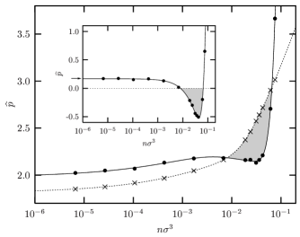
Figure 1: Contributions to the osmotic coefficient $\widehat{p}$ as a function of counterion density $n$ for a bulk systems of parallel charged rods characterized by $r_{0}/\sigma=1$, $b/\sigma=1.042$, $\ell_{\operatorname{B}}/\sigma=1$, and $v=3$. The heavy dots and crosses represent the non-electrostatic contribution (kinetic and excluded volume) and the negative of the electrostatic contribution, respectively (the curves are guides to the eye). The inset shows the total osmotic coefficient, and the limiting value of infinite dilution $1/2\xi v\approx 0.174$ is indicated by an arrow.

Figure 1 shows our MD-results for the osmotic coefficient of bulk systems which are characterized by $r_{0}/\sigma=1$, $b/\sigma=1.042$, $\ell_{\operatorname{B}}/\sigma=1$, and $v=3$. The pressure is identified with the component of the stress tensor perpendicular to the rods DeHo01 , and its contributions coming from electrostatic and non-electrostatic ($i$.$\,e$., entropic and excluded volume) origin are plotted separately. It can be seen that within a density range from roughly $n=8\times 10^{-3}\sigma^{-3}$ to $6.5\times 10^{-2}\sigma^{-3}$, corresponding to rod separations between $6.8\,\sigma$ and $2.4\,\sigma$, the osmotic pressure is negative. If the rods were not forced to remain at fixed separations, they would phase separate, producing a condensate and a dilute phase.

Surprisingly, the electrostatic contribution (which is always negative and always favors contraction) shows no particular features in the regime where $\widehat{p}<0$. It rather appears that the negative pressure originates from a drop in the repulsive excluded volume contribution which is large enough such that the electrostatic contribution can win against the short range repulsion. This finding is consistent with earlier simulation results NiGu91 which used finitely replicated cells. A possible explanation of this phenomenon rests on the following tempting picture: The excluded volume contribution to the pressure stems from the force that ions exert on the oppositely charged rods. If the density increases, the rods come closer to each other and start to pull the ions away from their neighbors, thereby reducing this force. However, at too high concentrations rods will again repel by pushing onto each other via the ions in between. We will come back to this effect in Sec. IV.2.

An alternative explanation suggests that the condensed ions between two neighboring rods form a mutually interlocked pattern, which results in a lower Coulomb energy (compared to a homogeneous charge distribution) and which thus leads to attractions RoBl96 ; GrMa97 ; ArLe00 ; LeAr99 . Since each rod has six neighbors, this defines six “planes” in which one would have to look for a two-dimensional interlocking pattern. However, we were unable to find a corresponding structure in our simulated data that goes beyond a weakly developed first correlation hole, which on its own is not a sure sign for attractions as we will show in Sec. IV.3 for the case of two rods. This may partly be related to the small degree of arbitrariness in the definition of the planes, but there is also a physical explanation to consider. The systems are comparatively dense in the regime where attractions occur. It is therefore likely that close ions are correlated irrespective of the plane they “belong” to—in other words, that those artificial planes are irrelevant for understanding the physics. It rather seems more reasonable to study the full three-dimensional correlations of the ions, as we will do in the following section.

III.2 Pair correlation function

If the radius of the rods and their mutual distance is smaller than the Bjerrum length, the electrostatic interaction of ions reaches beyond the nearest rod and the complete system of ions may form a three-dimensional correlated structure. More specifically, Shklovskii suggests Shk99a that in the case $r_{0}/b\ll v$, or equivalently $r_{0}/\ell_{\operatorname{B}}\ll v/\xi$, ions could form such a structure on the background of the rods, which for very high coupling can be described as a three-dimensional Wigner crystal (or at least as a strongly correlated liquid). We tested this assumption by computing the usual pair correlation function $g(r)$ for the systems above which showed negative pressure. Before we discuss the results, a few general remarks are appropriate.

If the ions form a three-dimensional crystal structure, there will be a typical minimum distance between them which should scale like one over the third root of the counterion density . However, there is a second important length scale, which is the separation of the rods and which is easily seen to scale as one over the square root of the counterion density. Hence, whatever the details of the actual ionic structure are, if one measures a characteristic length varying like $n^{-1/3}$, it can be viewed as a bulk correlated liquid property, while a length varying like $n^{-1/2}$ is rod-imposed.

In Fig. 2 we present results for the system studied above in the density range $0.02\,\sigma^{-3}\ldots 0.1\,\sigma^{-3}$, which corresponds to the high-density range in which the osmotic pressure was found to be negative. The dashed curve shows the pair correlation $g(r)$ at the density $n=4.25\times 10^{-2}\sigma^{-3}$, which is at the minimum of the osmotic coefficient in Fig. 1. A pronounced oscillatory structure is clearly visible. The inset shows the position of the first maximum as a function of density in a double logarithmic plot (open circles). In this range the data suggest a power law with exponent $-0.48$, which is close to the value expected for a rod-imposed structure. In fact, the oscillations in $g(r)$ simply reflect the periodicity of the array of rods.

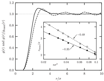
Figure 2: Pair correlation function $g(r)$ for the bulk system from Fig. 1 at a counterion density $n=4.25\times 10^{-2}\sigma^{-3}$ (dashed line). The solid line is the ratio between this $g(r)$ and $g_{\operatorname{rand}}(r)$ (see text). The inset shows a double logarithmic plot of the position of the first maximum of $g(r)$ (open circles) and $g(r)/g_{\operatorname{rand}}(r)$ (full circles) as a function of density; the slopes are indicated.

In order to extract actual inter-ionic correlations from the simulations, the imposed periodic inhomogeneity of the ion density has to be removed. One way of doing this is as follows: The pair correlation function is the probability of finding an ion at a distance $r$ from another ion relative to the probability of finding an ion at the same distance in a random ($i$.$\,e$., noninteracting, “ideal gas”) system at the same average density. In the present case it would be sensible to normalize not by a random homogeneous system but by a random inhomogeneous system, $i$.$\,e$., a system in which there are no inter-ionic correlations but the spatially varying ion density is preserved. This can be easily accomplished in the following way: In each configuration move every ion a random distance (between $0$ and $\sqrt{3}L$) along the direction of the rods. This does not change the inhomogeneous one-particle distribution, but completely destroys all two-particle correlations. Then compute the pair correlation function of this randomized system, $g_{\operatorname{rand}}(r)$. The ratio between the usual $g(r)$ and the randomized $g_{\operatorname{rand}}(r)$ now contains all information about inter-ionic correlations, but the imposed density inhomogeneity is divided out. This ratio is also plotted in Fig. 2 for the system at the density $n=4.25\times 10^{-2}\sigma^{-3}$ (solid line). Signs of correlations can again be seen, but the long range oscillatory part has been removed. The inset also shows the position of the first maximum of $g(r)/g_{\operatorname{rand}}(r)$ as a function of density (closed circles). The solid line has a slope of $-0.35$, which is more close to the exponent expected for a correlated three-dimensional ionic structure.

We see that the nature of correlations in this system is a subtle interplay between rod-imposed and inter-ionic contributions, and the latter are only identifiable once the former are divided out. The idea that a three-dimensional pattern of correlated ions forms on the structureless background of the rods is clearly too simple for the system under study. Furthermore, both correlations are comparatively weak, in the sense that the first maximum in $g(r)$ is fairly low, and the long range structure visible in the bare $g(r)$ is identical in $g_{\operatorname{rand}}(r)$ and thus is imposed by the external periodicity of the rods. The observed correlations are definitely much weaker than expected for a Wigner crystal or a strongly correlated liquid. If the ideas advocated in Ref. Shk99a ; Shk99b ; PeSh99 about the source of attraction are correct, the present analysis implies that a very low degree of correlations is already sufficient or, in other words, the Wigner crystal picture holds way beyond the ground state. This of course provokes the questions “Why?” and “How far beyond?”.

The above analysis does not directly explain our earlier finding that the occurrence of a negative pressure is ultimately related to a sudden drop in the repulsive excluded volume forces. One may speculate that the electrostatic part of the pressure responds less sensitively than the short range LJ-part to a comparatively local ordering as observed in Fig. 2, but additional studies would be needed to support this.

IV One pair of rods

The Wigner crystal picture is ultimately based on energetic arguments, it does not provide a direct “mechanical” explanation for why correlations actually produce an attractive force. To answer this question, these correlations have to be studied in more detail. However, the bulk system is not necessarily the easiest case: The relevant observable is the pressure, which is less direct than a force, and the more complex geometry complicates the definition of suitable and reasonably intuitive correlation functions. We therefore resort now to the interaction between two rods as well as the involved ionic correlations. As we have mentioned in the introduction, studying the pair interactions is not merely an alternative but also a complementary approach to studying the bulk system, since the forces in the latter cannot be decomposed into pair forces.

A pair of parallel rods has previously been investigated as a function of rod separation, which gives the distance dependence of the force GrMa97 ; ArSt99 ; AlLo00 ; DiCa01 and by integration the potential of mean force. In our work we supplement these results by studying the properties of the system at fixed distance as a function of Bjerrum length. This alternative scan is promising since unlike for bare charges the Bjerrum length does not simply enter as a prefactor of the interaction. Rather, its size will determine to what degree ions can be found close to the rods and how strongly they correlate with it as well as with each other, thereby influencing the nature of the force itself.

We studied three systems which differ in their values for rod radius and line charge density, as specified in Tab. 1, but we always kept the surface-to-surface distance between two rods around $2\,\sigma$, $i$.$\,e$., twice the diameter of a counterions, since this is a typical separation at which attractive forces have been found at sufficiently large Bjerrum length. The observables we measured were the force between the rods (split again into electrostatic and non-electrostatic origin) as well as various ionic correlation functions along and around the rods. The three studied systems will provide examples for qualitatively different behavior, but cannot predict detailed dependencies on key system parameters. For instance, the simulations in Ref. GrMa97 suggest that increasing the rod radius at fixed line charge density will ultimately remove repulsion, while increasing the line charge density at fixed rod radius will ultimately lead to attraction. However, present studies in this direction show a more complex behavior ArDe .

It is well known that the importance of correlations is strongly influenced by the valence of the counterions. However, this variable cannot be changed continuously. In contrast, increasing the Bjerrum length can be viewed as continuously increasing the strength of correlations and thereby studying in detail how they develop. Experimentally the Bjerrum length is a parameter whose change requires some effort, but it can be achieved for instance by a careful control of the solvent dielectric constant, as has been recently shown in an experimental study of the coil-globule transition of DNA MeKh99 .

IV.1 Force as a function of Bjerrum length

In a first step we study the force between the two rods by (separately) adding up all electrostatic and excluded volume forces that act on one rod and average over the simulation run (which typically means over about 3000 configurations separated by 2000 integration steps). Under periodic boundary conditions the total force on one rod originates not just from the neighboring rod, but also from all periodic images. However, we assume these contributions to be negligible in our case for the following reasons: For high Bjerrum length all ions are condensed onto the surface of the rods, implying that interactions of these essentially neutral objects ($i$.$\,e$., rods plus counterions) over a distance of the box length is much weaker than the direct interaction (compare the values for $s$ and $L$ in Tab. 1). It is not immediately clear that this remains valid in the limit $\ell_{\operatorname{B}}\rightarrow 0$, but in this case our data are always asymptotic to the analytical expression for the electrostatic force between two charged lines (see below), which implies that the images can be neglected as well.

One may ask why we used periodic boundary conditions in the first place, if we want images to be irrelevant. The answer is of course that the images along the direction of the rod are important, since they render the rods infinitely long—or stated differently: remove end effects. Periodic replication perpendicular to the axis of the rods is an unwanted but acceptable (since controllable) side effect imposed by the use of traditional Ewald schemes, in which it is not trivial to switch off periodicity in a specific direction. However, the latter can be achieved quite easily by using a one-dimensional version of MMM StSp01 ; ArHo01a ; ArHo01b , compare Sec.II, and we will also present data obtained by this second method.

Motivated by our observations in bulk simulations we also look at the components of the force originating from electrostatic and excluded volume interactions. Let us start with a few general remarks concerning what to expect. For $\ell_{\operatorname{B}}=0$ there is no electrostatic interaction between the rods, and the only possible source of interaction is a depletion attraction AsOo54 generated by the excluded volume of the (at $\ell_{\operatorname{B}}=0$ effectively uncharged!) ions . When slightly increasing the Bjerrum length, the two rods will feel an unscreened Coulomb repulsion, since for $\xi v<1/2$ ions will remain unbound Man69 . The force per unit length is then given by

$$\beta F\;\stackrel{{\scriptstyle\ell_{\operatorname{B}}\rightarrow 0}}{{=}}\;\frac{2\ell_{\operatorname{B}}}{b^{2}s},$$ (3)

$i$.$\,e$., proportional to Bjerrum length. In other words, in this regime the Bjerrum length still acts as a prefactor determining the strength of the interaction. Upon further increase of $\ell_{\operatorname{B}}$ ion condensation and subsequent correlations set in, resulting in nontrivial $F$-$\ell_{\operatorname{B}}$-curves (see below). However, in the limit $\ell_{\operatorname{B}}\rightarrow\infty$ everything becomes simple again: The counterions will ultimately assume a “ground state” configuration which will no longer change upon further increase of $\ell_{\operatorname{B}}$ (only fluctuations around the ground state will become weaker). Hence, the electrostatic force (and as an indirect consequence also the excluded volume force) will again be proportional to $\ell_{\operatorname{B}}$. However, the constant of proportionality cannot be predicted from these considerations—not even its sign. In the following we will plot the force per unit length and use the convention that a positive sign denotes repulsion, while a negative sign denotes attraction.

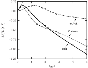
Figure 3: Force between two rods of system 1 from Tab. 1 as a function of Bjerrum length $\ell_{\operatorname{B}}$. Total force, excluded volume contribution and electrostatic contribution are represented by “$\cdot$” on a solid line, “$+$” on a dashed line, and “$\times$” on a dotted line, respectively. The fine dashed line indicates the limiting behavior from Eqn. (3). Positive forces denote repulsion, negative attraction. Measured values are indicated by the symbols, the lines should merely guide the eye.

Fig. 3 shows the result for system 1 (for notation see Tab. 1), which consists of rods having the same diameter as the ions and the same separation as in the system from Fig. 1 showing the most negative pressure. For small Bjerrum length the force is given by Eqn. (3). However, if $\xi v>1/2$ ($i$.$\,e$., $\ell_{\operatorname{B}}>0.17\,\sigma$ the present case) Manning condensation will set in on the two-rod system. Since ions will condense preferentially between the rods, they reduce the electrostatic repulsion, but at the same time produce an outward pressure due to their excluded volume.

Provided the excluded volume contribution to the interaction is not yet substantial, a description of the system using Poisson-Boltzmann (PB) theory can work up to this Bjerrum length. Indeed, the PB equation can be solved exactly in this geometry ImOn59 ; OhIm60 , but the analytical solution (in terms of hypergeometric functions) is extremely complicated. One particularly direct result however (exact for infinitely thin rods) is that if the two-rod-system is below the Manning threshold, pure Coulomb repulsion ($i$.$\,e$., unmodified by the presence of counterions) is found asymptotically at large separation, while if each rod is at the Manning threshold, the Coulomb repulsion at large distances is reduced by a factor of 2. We mention aside that for the case of two rods (of arbitrary radius) and added salt the PB equation has been solved numerically Har98 , and analytical studies in the presence of salt exist within linearized PB theory BrMc73 , even for tilted rods BrPa74 .

Upon further increase in Bjerrum length the electrostatic force is seen to change sign at $\ell_{\operatorname{B}}/\sigma\approx 0.6$, and the total force becomes attractive beyond $\ell_{\operatorname{B}}/\sigma\approx 0.9$. While it is easy to imagine counterion distributions between the two rods that would lead to electrostatic attraction, those distributions are counteracted by both entropy and excluded volume interactions among the ions, since a high density between the rods is required. A mean-field treatment on the level of PB theory ImOn59 ; OhIm60 ; Har98 cannot resolve the issue because rigorous proves exist that the above situation must give repulsion Neu99 ; SaCh99 ; Tri00 —contrary to the actual observation, which is in agreement with earlier simulational works LyNo97 ; GrMa97 . It is clear that (on the level of the restricted primitive model of electrolytes) the attraction must hence be related to the existence of correlations between the ions. We will discuss a few of them in the following section.

For a Bjerrum length larger than $2.5\,\sigma$ the excluded volume part of the force becomes attractive as well. This is surprising, since it implies that there are still sufficiently many ions between the rods to induce electrostatic attraction, but they organize their positions such that they put less pressure on the rods than the ions located on the outward surfaces.

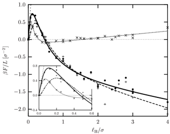
Figure 4: Force between two rods of system 2 as a function of Bjerrum length. The inset magnifies the initial region $\ell_{\operatorname{B}}\in[0;0.6]$. The line styles are the same as in Fig. 3.

In Fig. 4 we show the same Bjerrum-scan for system 2, which differs from the previous one in the following ways: The linear charge density is $6.78$ times larger, the rod radius is four times larger, and the rods are kept at a separation of $6\,\sigma$, which ensures that the surface-to-surface separation is again $2\,\sigma$. The generic behavior at small Bjerrum length is the same, but in this system a very pronounced difference occurs at larger values: Beyond $\ell_{\operatorname{B}}/\sigma\approx 1.5$ the electrostatic contribution to the force becomes repulsive and the total force is attractive only because of the excluded volume term. Note that together with the results discussed above this implies that a net attraction can occur both because electrostatic attraction overcomes excluded volume repulsion and because excluded volume interactions overcome an electrostatic repulsion. In the present case electrostatic repulsion is only weakly developed and numerical errors are large compared to the other two systems, but we have observed the same phenomenon in several other systems as well. Its characteristics will be discussed more thoroughly somewhere else ArDe . Even though this effect may appear counterintuitive, we want to remind the reader that minimizing the total energy of the ionic system at given rod separation does not imply that the electrostatic part of it gives rise to rod-rod-attractions.

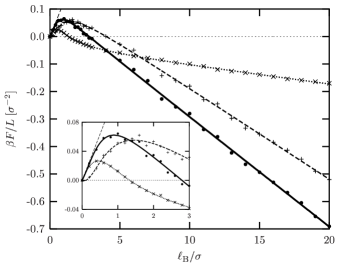
Figure 5: Force between two rods of system 3 as a function of Bjerrum length. The inset magnifies the initial region $\ell_{\operatorname{B}}\in[0;3]$. The line styles are the same as in Fig. 3.

Fig. 5 presents results for system 3, which compared to system 1 has an approximately $12.5$ times larger rod radius. The surface-to-surface separation is again maintained at $2\,\sigma$. The ratio $r_{0}/b\approx 6$ is close to that for DNA. Fixing the length scale via $b=b_{\text{DNA}}=1.7\,$Å implies a (somewhat small) ion diameter of $\sigma=1.63\,$Å . At the Bjerrum length $\ell_{\operatorname{B}}=7.14\,\text{\AA}=4.38\,\sigma$ (as appropriate for water at room temperature) the total force is attractive, and indeed it has been experimentally established that trivalent ions lead to attractive interactions between DNA strands WiBl79 ; BlWi80 ; WiBa80 ; RaPa92 ; PoRa94 ; Blo96 . Note also that just like in system 1 both contributions to the force are attractive at sufficiently high Bjerrum length; however, in system 3 the excluded volume part is stronger than the electrostatic part for values of $\ell_{\operatorname{B}}/\sigma$ larger than $\approx 6$.

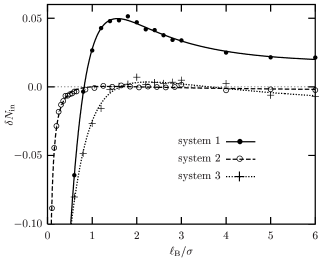
Figure 6: Relative imbalance $\delta N_{\text{in}}=(N_{\text{in}}-N_{\text{out}})/(N_{\text{in}}+N_{\text{out}})$ of ions between the rods and outside (see text) as a function of Bjerrum length for the three systems studied. Note that a positive $\delta N_{\text{in}}$ means that more ions are between the rods.

As we have mentioned above, the attraction between the rods due to electrostatic forces arises because ions condense preferentially between the rods. A straightforward measure for this imbalance is provided by the following observable: Imagine two parallel planes, each containing the axis of one of the rods, whose distance equals the axial distance between the rods. These planes divide space into a region “between” the rods and two disjunct regions “outside”. Denote by $N_{\text{in}}$ and $N_{\text{out}}$ the number of counterions in the region “between” and “outside”, respectively, and define the relative ionic excess between the rods as $\delta N_{\text{in}}=(N_{\text{in}}-N_{\text{out}})/(N_{\text{in}}+N_{\text{out}})$. This observable is plotted in Fig. 6 as a function of Bjerrum length for systems 1, 2 and 3. For small Bjerrum length $\delta N_{\text{in}}$ is negative, since ions are not condensed and the outside region is larger. As ion condensation sets in at increasing $\ell_{\operatorname{B}}$, $\delta N_{\text{in}}$ also increases until it reaches 0, the point at which the inside and outside numbers are balanced. For system 1, $\delta N_{\text{in}}$ becomes strongly positive afterwards, showing that there are more ions between the rods than outside, but it decreases again beyond $\ell_{\operatorname{B}}/\sigma\approx 1.5$, implying that this imbalance softens out. For system 2, $\delta N_{\text{in}}$ does not rise significantly above 0, but rather approaches this balance line at about $\ell_{\operatorname{B}}/\sigma\approx 1$. For system 3, $\delta N_{\text{in}}$ weakly rises above 0 at $\ell_{\operatorname{B}}/\sigma\approx 1.6$, but it again drops below at $\ell_{\operatorname{B}}/\sigma\approx 3.6$.

In all three systems the point at which the electrostatic force becomes attractive coincides roughly with the point at which a strongly negative imbalance $\delta N_{\text{in}}$ vanishes. However, one has to be careful in interpreting this observable: For system 1 the excluded volume repulsion between the rods vanishes beyond $\ell_{\operatorname{B}}/\sigma\approx 2.5$, but $\delta N_{\text{in}}$ is positive there, $i$.$\,e$., there are still more ions between the rods than outside. The attraction between the rods in system 2 is due to excluded volume forces, but the imbalance $\delta N_{\text{in}}$ is essentially 0. Hence, attraction occurs not due to a simple density difference. In the following section we will therefore also study the azimuthal distribution of ions in some more detail as well as the question how close the ions actually come to the rods.

Let us close our discussion of forces with the following observation. Compared to system 1 the density of surface charges $\varsigma$ is $12.5$ times lower in system 3, but the total force becomes attractive at $\ell_{\operatorname{B}}/\sigma\approx 2.9$, which is only $3.2$ times larger than for system 1. Rouzina and Bloomfield RoBl96 use the two-dimensional plasma parameter $\Gamma_{2}=\ell_{\operatorname{B}}v^{3/2}\varsigma^{1/2}$ as a measure for the strength of correlations and estimate that the onset of attraction should be expected at $\Gamma_{2}\approx 2$. This implies that the corresponding Bjerrum length scales inversely proportional to the square root of the surface charge density. For our simulations $\Gamma_{2}\approx 2.58$, $1.83$ and $2.35$ for systems 1, 2 and 3 at the onset of attraction, which agrees remarkably well with their estimate.

IV.2 Azimuthal correlations

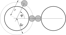
Figure 7: Geometry for the definition of the azimuthal correlation function $g(\varphi|\delta r)$. It is proportional to the probability density of finding a counterion at the angle $\varphi$ relative to the other rod within a condensation distance of at most $\delta r$. The normalization is such that $g=1$ corresponds to the average density, or stated differently, the average of $g$ is $1$.

The previous sections have revisited the importance of ionic correlations for the nature of the force between two charged rods, and in the following we will present measurements of a few of them. We start with an ion-rod correlation that answers the question how the ions distribute around a rod relative to the position of the other rod. Fig. 7 illustrates our definition of the correlation function. Denote the position of a counterion relative to rod 1 in polar coordinates $r$ and $\varphi$, such that $\varphi=0$ corresponds to the direction towards rod 2. We define $g(\varphi|\delta r)$ to be $2\pi$ times the probability density of finding an ion at the angle $\varphi$, given that its separation from rod 1 is at most $\delta r$. Note that this implies that the mean value of $g(\varphi|\delta r)$ (when averaged over $\varphi$) is 1. Obviously, $g(\varphi|\delta r)$ is periodic in $\varphi$ with period $2\pi$. At first we will choose $\delta r$ as large as possible, $i$.$\,e$., half the rod separation $s$. We want to mention that for $\delta r\rightarrow r_{0}$ this function is essentially the rod-analog of the density resolved by the polar angle for the spherical case studied in Ref. AlDa98 .

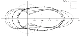
Figure 8: Polar plot of azimuthal correlation functions $g(\varphi|s/2)$ for system 1. The particular Bjerrum lengths are indicated. The neighboring rod is assumed to be located to the right side. The normalization is such that the average value of $g$ is equal to 1 (indicated by the dotted circle). Measured values (dots) are only indicated for the case $\ell_{\operatorname{B}}=1\,\sigma$.

Figure 8 shows a polar plot of $g(\varphi|s/2)$ for system 1. The Bjerrum length is varied between $1\,\sigma$ and $5\,\sigma$. Compare also the corresponding force-plot from Fig. 3. Several things can be observed: ($i$) The azimuthal correlation function is largest in the direction towards the other rod. ($ii$) There exists a “second tide” on the side opposing the other rod. ($iii$) The elongation of $g(\varphi|s/2)$ along the line joining the two rods increases with increasing Bjerrum length. ($iv$) The larger than average $g$ at $\varphi=0$ and maybe $\varphi=\pi$ is balanced by a less than average $g$ in the transverse direction. ($v$) While $g(0|s/2)$ is always larger than $1$, $g(\pi|s/2)$ is smaller than $1$ for sufficiently small Bjerrum length, but ultimately rises above $1$ as well.

As can be seen from Fig. 3, all five systems presented in Fig. 8 feature a net attraction, but for the systems with $\ell_{\operatorname{B}}/\sigma=1$ and $2$ the excluded volume part is still repulsive. It is unfortunately difficult to directly relate this finding to the shape of the azimuthal correlation function, since the position of the ions are of course relevant for both electrostatic and excluded volume forces, which are opposite and show a different distance dependence. We come back to this issue below, when we discuss the dependence on $\delta r$.

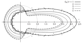
Figure 9: Same plot as in Fig. 8 for system 3. Measured values (dots) are only indicated for the case $\ell_{\operatorname{B}}=1\,\sigma$.

Fig. 9 shows exactly the same five correlation functions for system 3. This system differs from system 1 “only” by a $12.5$ times larger rod radius, but the shape of the correlation functions is quite different. The second peak at $\varphi=\pi$ has given way to two new peaks emerging somewhat beyond $\pi/2$, while the ion density at $\varphi=\pi$ is below average. The fact that the peak at $\varphi=0$ decreases upon increasing Bjerrum length can be traced back to the normalization of $g$ and the fact that the total number of ions within the shell $r\leq s/2$ initially increases as $\ell_{\operatorname{B}}$ increases. At low Bjerrum length most of the condensed ions can be found between the rods. Upon increasing $\ell_{\operatorname{B}}$ the additionally condensed ions will occupy the other parts of the rod, thereby reducing the relative weight of the ones at $\varphi=0$. Once essentially all ions have condensed within the shell $r\leq s/2$, a larger Bjerrum length will only enhance the correlations and thereby make the peak at $\varphi=0$ larger again. We note that in the spirit of our mapping indicated above the azimuthal correlation function for ions around DNA would approximately be given by the curves for $\ell_{\operatorname{B}}/\sigma=4$ or 5.

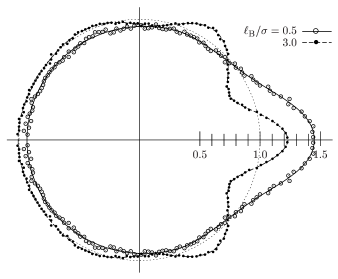
Figure 10: Same plot as in Fig. 8 for system 2. Measured values for $\ell_{\operatorname{B}}/\sigma=0.5$ and $\ell_{\operatorname{B}}/\sigma=3.0$ are indicated as open circles ($\circ$) and dots ($\cdot$), respectively. The lines should merely guide the eye.

In Fig. 10 we show $g(\varphi|s/2)$ for two versions of system 2. This system has a rod radius $4$ times larger than system 1 and a line charge density about 6.8 times larger. For a Bjerrum length of $\ell_{\operatorname{B}}=0.5\,\sigma$, for which the total force between the rods approximately vanishes (see Fig. 4), a pronounced peak in $g(\varphi|s/2)$ towards the neighboring rod as well as a slightly smaller than average counterion density on the opposite side is visible. Just as for system 3, upon increasing the Bjerrum length $g(\varphi|s/2)$ does not merely “intensify” its features but develops a qualitatively new structure. In addition to the main correlation peak at $\varphi=0$, five new peaks show up, roughly at multiples of $60^{\circ}$. This occurrence of additional peaks is a common phenomenon in usual liquids as correlations increase. However, in the present case we have the additional constraint that $g(\varphi|\delta r)$ is periodic in $\varphi$ and obviously an even function, which restricts the locations of these peaks. While for a flat two-dimensional system the position of peaks in the pair correlation function is solely determined by the density of charges ($\varsigma^{-1/2}$ is the only available length scale), in a curved geometry two more effects play a role: first, the radius of curvature appears as a new length scale, and second, topological constraints require the function to close upon itself as in the case above. Particularly the latter observation suggests that there are situations in which this matching works “automatically” whereas in other situations it leads to a frustration. This may favor counterion conformations which relax these constraints ($e$.$\,g$. helices) and influence the strength of the rod-rod-interaction.

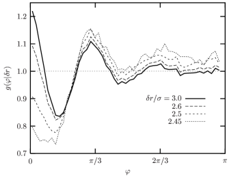
Figure 11: Azimuthal correlation functions $g(\varphi|\delta r)$ for the system 2 with $\ell_{\operatorname{B}}=3\,\sigma$ (see also Fig. 10) for different values of $\delta r$. Note in particular that for decreasing $\delta r$ the peak at $\varphi=0$ turns into a correlation hole.

We conclude our discussion of the azimuthal correlation function by discussing its dependence on $\delta r$. This variable determines which counterions are taken into account for computing the density as a function of $\varphi$. If $\delta r$ gets smaller, the focus is on ions that are more closely in contact with the rod. Fig. 11 shows a plot of $g(\varphi|\delta r)$ for system 2 with $\ell_{\operatorname{B}}=3\,\sigma$. The bold solid line is the same curve as shown in Fig. 10 ($i$.$\,e$., $\delta r=s/2=3\,\sigma$), only plotted in a Cartesian way. The other three curves correspond to successively smaller values of $\delta r$. We would like to draw attention to the fact that the peak at $\varphi=0$ gives way to a correlation hole. While $g(0|\delta r)$ decreases upon reduction of $\delta r$, $g(\pi|\delta r)$ increases. This is important since the ions most closely in contact with the rod produce the strongest excluded volume force. Fig. 11 thus shows that ions very close to the surface of the rods are more likely to push them inwards rather than outwards. Note that this particular system is special in that the attractive forces have been found to originate from the excluded volume term, see Fig. 4. A similar $\delta r$-analysis for system 1 in the strongly attractive regime at $\ell_{\operatorname{B}}=20\,\sigma$ does not show this effect (data not shown). As $\delta r$ gets smaller than $1.0\,\sigma$, the peaks at $\varphi=0$ and $\varphi=\pi$ start decreasing and rising, respectively, but the former does not turn into a correlation hole. The same finding applies to system 3 in the attractive regime at $\ell_{\operatorname{B}}=5\,\sigma$. However, note also that in the latter two systems electrostatics is the dominant reason for attraction. Unfortunately, effects at small $\delta r$ are difficult to observe, since the small number of ions at these close distances impedes a good statistics.

We want to remark that a similar correlation hole has been previously observed in the spherical case and has been termed an electrostatic depletion effect AlDa98 . Observe that in our case this effect is only visible if one focuses on ions very close to the surface of the macroion—the total amount of ions between the macroions is above average, which contradicts the depletion picture.

IV.3 Ion interlocking

It has previously been suggested that the ionic correlations in the case of attracting rods take the form of an interlocked pattern in the plane between the rods RoBl96 ; GrMa97 ; ArLe00 ; LeAr99 . In this section we present first measurements of these kind of correlations under off-lattice conditions. It turns out that alternating charge-asymmetries indeed exist, but they are remarkably weakly pronounced and fairly short ranged. We also investigate their relevance for the attraction.

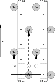
Figure 12: Scheme of a possible “ground state” of the two rod systems, showing ion interlocking. The relative position of three kinds of condensed counterions with respect to a condensed ion between the rods give rise to three different correlation functions, as discussed in the text.

Fig. 12 envisages a tentative “ground state” for system 1 from Tab. 1. We have previously deduced from Fig. 8 that in the limit of high Bjerrum length the ions are essentially either at $\varphi=0$ or $\varphi=\pi$. On each rod, every three monomers a trivalent counterion is condensed. The ions between the rods form an interlocked pattern that also gets imprinted on the ions located on the opposite side of the rods. Such a pattern suggests the definition of the following three pair correlation functions, as indicated in Fig. 12: Given an ion, that is condensed on one rod and sits between the two rods, what is the probability of having a second ion at a distance $z$ along the rods that is condensed (1) on the opposing rod and also between the rods, (2) on the same rod and also between the rods, and (3) on the same rod, but facing outward? With the usual normalization to $1$ at large distance, let us call these three functions $g_{1}(z)$, $g_{2}(z)$ and $g_{3}(z)$, respectively. We only consider ions whose center has a distance of less than $\sigma/2$ from the common plane of the rods.

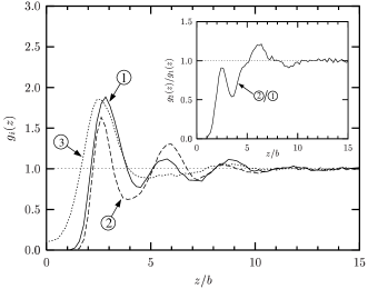
Figure 13: Interlocking correlation functions $g_{1}(z)$ (solid line), $g_{2}(z)$ (dashed line) and $g_{3}(z)$ (dotted line) as defined in Fig. 12 and the text for system 1 with Bjerrum length $\ell_{\operatorname{B}}=5\,\sigma$. The inset shows the ratio $g_{2}(z)/g_{1}(z)$.

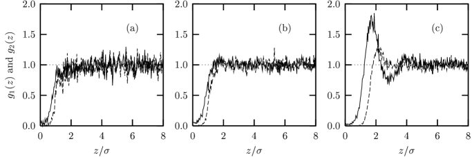
Figure 14: Interlocking correlation functions $g_{1}(z)$ (solid line) and $g_{2}(z)$ (dashed line) for system 2 with three values of the Bjerrum length: (a) $\ell_{\operatorname{B}}=0.125\,\sigma$, (b) $\ell_{\operatorname{B}}=0.5\,\sigma$, and (c) $\ell_{\operatorname{B}}=3\,\sigma$.

Fig. 13 shows the result of a measurement of these three correlation functions for system 1 with $\ell_{\operatorname{B}}=5\,\sigma$. Pronounced correlations are clearly visible, but their range is comparatively short. Structural features in the correlation function $g_{3}$ are much weaker developed. The reason for this is that the ionic density outside the rods is lower than between them, and the structure arises from a weak “transfer” of the correlations of $g_{1}$ and especially $g_{2}$.

It may seem surprising that not just $g_{1}(z)$ but also $g_{2}(z)$ has its first peak at $z\approx 3b$. The reason for this is that just as for the three-dimensional pair correlation function discussed in Sec. III.2 a fair amount of long-ranged periodicity in the $g_{i}(z)$ arises due to an external imprinting. Here it is the fact that charge neutrality essentially requires 1 trivalent ion per rod every $3b$. A visual inspection of typical ion configurations also shows that the system is still far from a highly ordered ground state as envisaged in Fig. 12. In particular, for $\ell_{\operatorname{B}}/\sigma=5$ the imbalance $\delta N_{\text{in}}$ presented in Fig. 6 has a value of about 0.022, which implies that the average density between the rods is about 5% higher than outside. These additional ions have to be put somewhere and clearly destroy the simple groundstate from Fig. 12. Together these findings imply that $3b$ is also a typical distance that has to be expected for $g_{2}$, but observe also that the peak in $g_{2}(z)$ at $z\approx 3b$ is less pronounced than the one for $g_{1}(z)$. In fact, the terminology “interlocking” suggests that we should be interested in the relative charge asymmetries along the rods. A better measure would therefore be the ratio between the two inner correlation functions, as is shown in the inset of Fig. 13. For $z\rightarrow 0$ the ratio $g_{2}(z)/g_{1}(z)$ approaches 0, since the correlation hole of $g_{2}(z)$ at $z=0$ is of course more pronounced than that for $g_{1}(z)$. The small peak shortly before $z=3b$ indicates the high probability for this distance as discussed above, but the fact that the peak value is below 1 means that such a value occurs more likely for ions belonging to different rods. A somewhat broader peak can be seen around $z\approx 6b$. It has its value above 1, indicating that this distance occurs preferentially for ions on the same rod. Beyond $z=10b$ no significant structure is visible.

Together these findings show that ion interlocking does indeed occur, but that it is again superimposed by “trivial” periodicities along the rods and that its extension along the rods is fairly weak. For increasing Bjerrum length the above features get more pronounced and the oscillatory structure extends towards larger separations, while for decreasing Bjerrum length the features diminish. At $\ell_{\operatorname{B}}=1\,\sigma$, at which the total force is approximately $0$, the only remaining feature of all three correlation functions is the correlation hole at $z=0$ (data not shown), which survives at even smaller values for $\ell_{\operatorname{B}}$.

We would like to emphasize that this correlation hole at $z=0$ is not sufficient to entail attractive forces. This is important for the following reason: In the Wigner crystal approach the correlation energy of an ion can be well approximated by its interaction energy with the counter-charge within its correlation hole, which turns out to give the dominant contribution to the energy up to temperatures far beyond the crystallization Shk99b . This may give the impression that the existence of this first correlation hole is also sufficient for the appearance of attractive forces. Fig. 14 gives another illustration that this is not the case. The correlation functions $g_{1}$ and $g_{2}$ are plotted for system 2 for three values of the Bjerrum length $\ell_{\operatorname{B}}/\sigma=0.125$, $0.5$ and $3$. As can be seen from Fig. 4, the first case corresponds to the strongest total repulsion, the second to an approximately vanishing net force and the third case to attraction. While the correlation functions in the first two cases are very similar, in the third case pronounced interlocking is observed.

One word of caution should be addressed to the numerous theories which apply the interlocking picture to DNA-like systems. Our simulations show that the net attractive force in System 3 around $\ell_{\operatorname{B}}/\sigma\approx 4-5$ is only weak compared to the other two systems, and thus an interlocking pattern at theses values of $\ell_{\operatorname{B}}$ is basically invisible.

V Summary, questions and outlook

We have revisited the phenomenon of attractive interactions in systems of charged rods in the presence of multivalent counterions. Within bulk systems this effect is seen as a negative osmotic pressure. Separating between ($i$) the electrostatic and ($ii$) the entropic plus excluded volume component unveils the key role played by the short range repulsive forces. We further explored these components by measuring their contribution to the force between two parallel charged rods as a function of Bjerrum length $\ell_{\operatorname{B}}$. An important result is that an overall attraction can be due to $(i)$ both electrostatic and excluded volume forces bringing the rods together, ($ii$) an electrostatic attraction overcoming excluded volume repulsion, and ($iii$) a short range excluded volume force pushing the rods together against an electrostatic repulsion. The excluded volume induced attraction can occur even if the average density between the rods is higher than outside, hence it is not a simple depletion mechanism. This suggests that there exists more than one mechanism for attraction between rods. It is the subtle interplay between several effects which ultimately determine the total force. We have shown that this crucially depends on the parameters of the system, like the line charge density or the rod radius.

We also presented measurements of various ionic correlation functions. For the bulk systems the scaling of the first peak of the three-dimensional pair correlation function indicates the existence of a three-dimensional correlated liquid, but only if one corrects for trivial effects due to the inhomogeneous average ion density. The assumption of a correlated liquid forming on the background of the rods is thus too simple. If the attractive interactions are still to be explained on the basis of the weak and masked three-dimensional correlations, this would imply that the Wigner crystal idea remains useful far beyond the ground state.

For the two rod case we studied the distribution of ions around one rod relative to the other. We always found a correlation peak towards the other rod, but the rest of the distribution depends sensitively on Bjerrum length, line charge density and the rod radius. On the far side of the rod there exists a correlation hole at low Bjerrum length, which may turn into a peak at increasing Bjerrum length. Also, secondary peaks can appear at a certain angle with respect to the rod-rod direction. The periodicity of the azimuthal correlation function implies commensurability constraints, which influence the structure. The azimuthal correlation function was also shown to depend on the condensation radius $\delta r$. It has been demonstrated for one system that the peak at $\varphi=0$ can turn into a correlation hole if one focuses on the ions most close to the rod. While this is important for the direction of the short range repulsive forces, it is presently unclear under which circumstances this effect occurs.

We finally confirmed the recently proposed picture of ions mutually interlocking between the rods. The closest ions along the direction of the rod have a tendency to be condensed on different rods, even though defects in this structure occur quite frequently. In agreement with earlier observations on discretized models DiCa01 this structure is remarkably short ranged. While attractive interactions have been found for all cases in which a first correlation peak is discernible, the mere existence of a first correlation hole was demonstrated to be insufficient.

The phenomena observed in our molecular dynamics simulations also give rise to several new questions, for instance: How can one predict the relative contribution of electrostatic and short range forces to the net interaction between rods? The structural changes in the azimuthal correlation functions result from usual pair correlation functions being “wound up” around the rod. In consequence, the condensed ions predominantly push or pull from specific directions, not necessarily aligned with the direction joining the rods. What effects on the net force does this have? Under which circumstances do the ions between the rods get pulled away from the surface, and when is this the dominant force of attraction? Further studies along these lines are currently under way.

VI Acknowledgments

We would like to thank B. Jönsson and B. Shklovskii for stimulating discussions. MD thanks the German Science Foundation (DFG) for financial support under grant De 775/1-1. CH wants to thank the “Zentrum für Multifunktionelle Werkstoffe und Miniaturisierte Funktionseinheiten”, grant BMBF 03N 6500.

References

- (1) B. V. Derjaguin and L. D. Landau, Acta Phys. Chim. URSS 41, 663 (1941).
- (2) E. J. W. Verwey and J. T. G. Overbeek, Theory of the Stability of Lyophobic Colloids, Elsevier, Amsterdam (1948).
- (3) F. Oosawa, Biopolymers 6, 1633 (1968).
- (4) F. Oosawa, Polyelectrolytes, Marcel Dekker, New York (1971).
- (5) G. N. Patey, J. Chem. Phys. 72, 5763 (1980).
- (6) D. Bratko and V. Vlachy, Chem. Phys. Lett. 90, 434 (1982).
- (7) L. Guldbrand, B. Jönsson, H. Wennerström, and P. Linse, J. Chem. Phys. 80, 2221 (1984).
- (8) B. Svensson and B. Jönsson, Chem. Phys. Lett. 108, 580 (1984).
- (9) L. Guldbrand, L. G. Nilsson, and L. Nordenskiöld, J. Chem. Phys. 85, 6686 (1985).
- (10) L. G. Nilsson, L. Guldbrand, and L. Nordenskiöld, Mol. Phys. 72, 177 (1991).
- (11) J. P. Valleau, R. Ivkov, and G. M. Torrie, J. Chem. Phys. 95, 520 (1991).
- (12) A. P. Lyubartsev, L. Nordenskiöld, J. Phys. Chem. 101, 4335 (1995).
- (13) N. Grønbech-Jensen, R. J. Mashl, R. F. Bruinsma, and W. M. Gelbart, Phys. Rev. Lett. 78, 2477 (1997)
- (14) A. P. Lyubartsev, J. X. Tang, P. A. Janmey, and L. Nordenskiöld, Phys. Rev. Lett. 81, 5465 (1998).
- (15) E. Allahyarov, I. D’Amico, and H. Löwen, Phys. Rev. Lett. 81, 1334 (1998).
- (16) N. Grønbech-Jensen, K. M. Beardmore, and P. Pincus, Physica A 261, 74 (1998).
- (17) M. J. Stevens, Phys. Rev. Lett. 82, 101 (1999).
- (18) P. Linse and V. Lobaskin, Phys. Rev. Lett. 83, 4208 (1999).
- (19) P. Linse, J. Chem. Phys. 113, 4359 (2000).
- (20) E. Allahyarov and H. Löwen, Phys. Rev. E 62, 5542 (2000).
- (21) M. Deserno, C. Holm, and S. May, Macromolecules 33, 199 (2000).
- (22) R. Messina, C. Holm, and K. Kremer, Phys. Rev. Lett. 85, 872 (2000).
- (23) M. Lozada-Cassou, J. Phys. Chem. 87, 3279 (1983).
- (24) C. W. Outhwaite and L. B. Bhuiyan, J. Chem. Soc. Farad. Trans. 2 79, 707 (1983).
- (25) R. Kjellander and S. Marčelja, Chem. Phys. Lett. 112, 49 (1984).
- (26) E. Gonzales-Tovar, M. Lozada-Cassou, and D. Henderson, J. Chem. Phys. 83, 361 (1985).
- (27) R. Kjellander and S. Marčelja, J. Chem. Phys. 82, 2122 (1985).
- (28) R. Kjellander and S. Marčelja, J. Chem. Phys. 88, 7129 (1988).
- (29) R. Kjellander and S. Marčelja, J. Chem. Phys. 88, 7138 (1988).
- (30) M. Lozada-Cassou and D. Henderson, Chem. Phys. Lett. 127, 392 (1986).
- (31) M. Lozada-Cassou and E. Díaz-Herrera, J. Chem. Phys. 92, 1194 (1990).
- (32) C. W. Outhwaite and L. B. Bhuiyan, Mol. Phys. 74, 367 (1991).
- (33) T. Das, D. Bratko, L. B. Bhuiyan, and C. W. Outhwaite, J. Phys. Chem. 99, 410 (1995); 107, 9197 (1997).
- (34) H. Greberg and R. Kjellander, J. Chem. Phys. 108, 2940 (1998).
- (35) M. Deserno, F. Jiménez-Ángeles, C. Holm, and M. Lozada-Cassou, J. Phys. Chem. B 105, 10983 (2001).
- (36) R. Groot, J. Chem. Phys. 95, 9191 (1990).
- (37) R. Penfold, B. Jönsson, S. Nordholm, and C. E. Woodward, J. Chem. Phys. 92, 1915 (1990).
- (38) Z. Tang, L. E. Scriven, and H. T. Davis, J. Chem. Phys. 97, 494, 9258 (1992).
- (39) R. Penfold, B. Jönsson, and S. Nordholm, J. Chem. Phys. 99, 497 (1993).
- (40) A. Diehl, M. N. Tamashiro, M. C. Barbosa, and Y. Levin, Physica A 274, 433 (1999).
- (41) M. C. Barbosa, M. Deserno, and C. Holm, Europhys. Lett. 52, 80 (2000).
- (42) R. Podgornik and B. Žekš, J. Chem. Soc. Faraday Trans. 2 84, 611 (1988).
- (43) R. D. Coalson and A. Duncan, J. Chem. Phys. 97, 5653 (1992).
- (44) R. R. Netz and H. Orland, Eur. Phys. J. E 1, 203 (2000)
- (45) A. G. Moreira and R. R. Netz, Europhys. Lett. 52, 705 (2000).
- (46) R. R. Netz, Eur. Phys. J. E 5, 557 (2001).
- (47) B.-Y. Ha and A. J. Liu, Phys. Rev. Lett. 79, 1289 (1997).
- (48) R. M. Nyquist, B.-Y. Ha, and A. J. Liu, Macromolecules 32, 3481 (1999).
- (49) I. Rouzina and V. A. Bloomfield, J. Phys. Chem. 100, 9977 (1996).
- (50) F. J. Solis and M. Olvera de la Cruz, Phys. Rev. E 60, 4496 (1999).
- (51) B. I. Shklovskii, Phys. Rev. Lett. 82, 3268 (1999).
- (52) B. I. Shklovskii, Phys. Rev. E 60, 5802 (1999).
- (53) V. I. Perel and B. I. Shklovskii, Physica A 274, 446 (1999).
- (54) J. J. Arenzon, J. F. Stilck, and Y. Levin, Eur. Phys. J. B 12, 79 (1999).
- (55) J. J. Arenzon, Y. Levin, and J. F. Stilck, Physica A 283, 1 (2000).
- (56) A. Diehl, H. A. Carmona, and Y. Levin, Phys. Rev. E 64, 011804 (2001).
- (57) A. W. C. Lau, D. Levine, and P. Pincus, Phys. Rev. Lett. 84, 4116 (2000).
- (58) A. W. C. Lau, P. Pincus, D. Levine, and H. A. Fertig, Phys. Rev. E 63, 051604 (2001).
- (59) L. Belloni, J. Phys.: Condens. Matter 12, R549 (2000).
- (60) B. Jönsson and H. Wennerström, “When ion-ion correlations are important in charged colloidal systems”, in: Proceedings of the NATO Advanced Study Institute on Electrostatic Effects in Soft Matter and Biophysics, ed. by C. Holm , Kluwer (2001).
- (61) R. W. Wilson and V. A. Bloomfield, Biochemistry 18, 2192 (1979).
- (62) V. A. Bloomfield, R. W. Wilson, D. C. Rau, Biophys. Chem. 11, 339 (1980).
- (63) J. Widom and R. L. Baldwin, J. Mol. Biol. 144, 431 (1980).
- (64) D. C. Rau and V. A. Parsegian, Biophys. J. 61, 246 (1992).
- (65) R. Podgornik, D. C. Rau, and V. A. Parsegian, Biophys. J. 66, 962 (1994).
- (66) V. A. Bloomfield, Current Opin. Struct. Biol. 6, 334 (1996).
- (67) O. Lambert, L. Letellier, W. M. Gelbart, and J. Rigaud, Proc. Nat. Acad. Sci. USA 97, 7248 (2000).
- (68) W. M. Gelbart, R. F. Bruinsma, P. A. Pincus, and V. A. Parsegian, Physics Today 53, 38 (2000).
- (69) B. V. R. Tata, M. Rajalakshmi, and A. K. Arora, Phys. Rev. Lett. 69, 3778 (1992).
- (70) K. Ito, H. Yoshida, and N. Ise, Science 263, 66 (1994).
- (71) B. V. R. Tata, E. Yamahara, P. V. Rajamani, and N. Ise, Phys. Rev. Lett. 78, 2660 (1997).
- (72) H. Yoshida, J. Yamanaka, T. Koga, T. Koga, N. Ise, and T. Hashimoto, Langmuir 15, 2684 (1999).
- (73) I. Sogami and N. Ise, J. Chem. Phys. 81, 6320 (1984).
- (74) R. van Roij and J.-P. Hansen, Phys. Rev. Lett. 79, 3082 (1997).
- (75) R. van Roij, M. Dijkstra, and J.-P. Hansen, Phys. Rev. E 59, 2010 (1999).
- (76) P. B. Warren, J. Chem. Phys. 112, 4683 (2000).
- (77) T. Palberg and M. Würth, Phys. Rev. Lett. 72, 786 (1994).
- (78) J. T. G. Overbeek, J. Chem. Phys. 87, 4406 (1987).
- (79) H. H. von Grünberg, R. van Roij, and G. Klein, Europhys. Lett. 55, 580 (2001).
- (80) M. Deserno and H. H. von Grünberg, Phys. Rev. E, in press.
- (81) M. Deserno, Ph.D. thesis, Universität Mainz, 2000, http://archimed.uni-mainz.de/pub/2000/0018/.
- (82) M. Deserno, C. Holm, and K. Kremer, in Physical Chemistry of Polyelectrolytes, Vol. 99 of Surfactant science series, edited by T. Radeva (Marcel Decker, New York, 2001), Chap. 2, pp. 59–110.
- (83) M. Deserno, C. Holm, Mol. Phys., (2002), in press.
- (84) G. S. Grest and K. Kremer, Phys. Rev. A 33, 3628 (1986).
- (85) J. D. Weeks, D. Chandler, and H. C. Andersen, J. Chem. Phys. 54, 5237 (1971).
- (86) R. W. Hockney and J. W. Eastwood, Computer Simulations using Particles, IOP, Bristol (1988).
- (87) M. Deserno and C. Holm, J. Chem. Phys. 109, 7678, 7694 (1998).
- (88) G. S. Manning, J. Chem. Phys. 51, 924, 934, 3249 (1969).
- (89) R. M. Fuoss, A. Katchalsky, and S. Lifson, Proc. Natl. Acad. Sci. USA 37, 579 (1951).
- (90) T. Alfrey, P. W. Berg, and H. Morawetz, J. Polym. Sci. 7, 543 (1951).
- (91) B. K. Klein, C. F. Anderson, and M. T. Record Jr., Biopol. 20, 2263 (1981).
- (92) M. Le Bret and B. H. Zimm, Biopolymers 23, 287 (1984).
- (93) L. Belloni, M. Drifford, and P. Turq, Chem. Phys. 83, 147 (1984).
- (94) R. Strebel, R. Sperb, Mol. Sim. 27, 61, (2001).
- (95) A. Arnold and C. Holm, Comp. Phys. Comm., in press; see also cond-mat/0202265.
- (96) A. Arnold and C. Holm, Chem. Phys. Lett. 354, 324 (2002).
- (97) A. A. Kornyshev, S. Leikin, J. Chem. Phys. 107, 3656 (1997); Erratum: J. Chem. Phys. 108, 7035 (1998); Proc. Nat. Acad. Sci. USA 95, 13579 (1998); Phys. Rev. Lett. 84, 2537 (2000); Phys. Rev. E 62, 2576 (2000); Phys. Rev. Lett. 86, 3666 (2001).
- (98) A. A. Kornyshev, S. Leikin, and S. V. Malinin, Eur. Phys. J. E 7, 83 (2002).
- (99) Y. Levin, J. J. Arenzon, and J. F. Stilck, Phys. Rev. Lett. 83, 2680 (1999).
- (100) A. Arnold, M. Deserno, and C. Holm, in preparation.
- (101) S. M. Mel’nikov, M. O. Khan, B. Lindman, and B. Jönsson, J. Am. Chem. Soc. 121, 1130 (1999).
- (102) S. Asakura and F. Oosawa, J. Chem. Phys. 22 ,1255 (1954).
- (103) N. Imai and T. Onishi, J. Chem. Phys. 30, 1115 (1959).
- (104) T. Ohnishi, N. Imai, and F. Oosawa, J. Phys. Soc. Japan 15, 896 (1960).
- (105) D. Harries, Langmuir 14, 3149 (1998).
- (106) S. L. Brenner and D. A. McQuarrie, J. Colloid Interf. Sci. 44, 298 (1973).
- (107) S. L. Brenner and V. A. Parsegian, Biophys. J. 14, 327 (1974).
- (108) J. Neu, Phys. Rev. Lett. 82, 1072 (1999).
- (109) J. E. Sader and D. Y. C. Chan, J. Colloid Interf. Sci. 213, 268 (1999).
- (110) E. Trizac, Phys. Rev. E 62, R1465 (2000).