Fractal entropy of a chain of nonlinear oscillators

Abstract

We study the time evolution of a chain of nonlinear oscillators. We focus on the fractal features of the spectral entropy and analyze its characteristic intermediate timescales as a function of the nonlinear coupling. A Brownian motion is recognized, with an analytic power-law dependence of its diffusion coefficient on the coupling.

I Introduction

A system composed of a large number of particles (generically) relaxes toward an equilibrium state that is independent of the details of the initial state. This is one of the fundamental hypotheses of statistical mechanics. However, from the point of view of Hamiltonian dynamics, the detailed features of the relaxation are not thoroughly understood. One of the unsolved fundamental questions is how equilibrium is approached when the underlying microscopic dynamics is sufficiently chaotic, without introducing any randomization or coarsegraining “by hand.”

After the pioneering work on the time evolution of nonintegrable systems FPU and ergodicity Sinai , it is now clear that several additional factors play a primary role in characterizing the dynamical evolution KAM ; Nekhoroshev ; Arnolddiff ; Lichtenberg . However, for a large number of particles the KAM argument becomes less effective Lichtenberg ; ParisiSFT and the Nekhoroshev bound Nekhoroshev for the equilibrium time appears too weak in comparison with numerical results. This scenario has motivated a number of numerical studies of Fermi-Pasta-Ulam-like models, in the attempt to clarify the dependence of the equilibrium time (defined in terms of suitable indicators) on the strength of the nonlinear terms and the number of particles Casetti97 . These studies yield stretched-exponential relaxation laws, enforcing the picture that macroscopic equilibrium could be built out of local ones Reigada02 .

The aim of this article is to investigate this issue by analyzing, both analytically and numerically, the dynamics of a chain of $N$ coupled anharmonic oscillators at intermediate timescales (for states that are close to equilibrium). One of our main results is that at these intermediate timescales the system performs a Brownian motion with a diffusion constant that can be accurately estimated and turns out to be analytically diverging in the coupling constant: as a consequence, a perturbative approach to this problem appears sensible.

II The system

We will study a Hamiltonian made up of an integrable part and a (small) nonlinear perturbation. This is a classical nonintegrable system, that does not possess enough integrals of motion. The conjugate variables are $(q,p)=(q_{1},...q_{N},p_{1},...,p_{N})$, where periodic boundary conditions $q_{N+1}=q_{1},\;p_{N+1}=p_{1}$ are understood. We take $N=2^{7}=128$, for convenience of the numerical algorithm (we observed no significant difference for larger $N$). The Hamiltonian ($\phi^{4}$ model) reads

$$H(q,p)=H_{0}(q,p)+gV(q),\quad(g>0)$$ (1)

$$H_{0}(q,p)=\sum_{i=1}^{N}\frac{1}{2}p_{i}^{2}+\frac{1}{2}m^{2}q_{i}^{2}+\frac{1}{2}\left(q_{i+1}-q_{i}\right)^{2},$$ (2)

$$V(q)=\sum_{i=1}^{N}\frac{1}{4}q_{i}^{4}.$$ (3)

The quadratic part $H_{0}$ is easily diagonalized by means of a discrete Fourier transform, in terms of the $2N$ normal variables $q_{\kappa},\ p_{\kappa}$, with $\kappa=(k,a)$, where $k=0,...,N/2$ and $a=0,1$, $a=0\;(a=1)$ corresponding to the cosine (sine) transform with wave number $k$. With this coordinate change $H_{0}$ becomes

$$H_{0}=\sum_{\kappa}E_{\kappa},\qquad E_{\kappa}=\frac{1}{2}p_{\kappa}^{2}+\frac{1}{2}\omega_{k}^{2}q_{\kappa}^{2},$$ (4)

with the frequency spectrum

$$\omega_{k}^{2} = m^{2}+2\left(1-\cos\left(\frac{2\pi k}{N}\right)\right),$$

$$m = \omega_{\mathrm{min}}\leq\omega_{k}\leq\omega_{\mathrm{MAX}}=\sqrt{4+m^{2}}.$$ (5)

In this article we always set $m^{2}\gtrsim 0.1$. The value of $m$ determines the width of the spectrum and has profound consequences on the dynamics, in particular at small nonlinearities: metastable states, like solitons and breathers, are born more easily at small $m$ and this can have drastic consequences, both at intermediate and large timescales of the equilibration process Reigada02 .

We integrated the Hamilton equations deriving from (1) via a fourth-order Runge-Kutta algorithm in double precision. Energy conservation is verified at least up to 1 part in $10^{7}$ during the whole running time. Such a precision is necessary in order to assure that the fluctuations due to numerical integrations be negligible with respect to the physical ones in which we are interested.

III Spectral entropy

From the numerically integrated solutions we analyze the behavior of the spectral entropy Casetti97

$$S(t)=-\sum_{\kappa}\frac{E_{\kappa}}{E_{0}}\ln\frac{E_{\kappa}}{E_{0}},$$ (6)

where $E_{0}=H_{0}$ is the unperturbed total energy. When $g=0$ all the $E_{\kappa}$s, and therefore $S$, are constant. As soon as the nonlinearity is switched on, $g>0$, the spectral entropy becomes a nontrivial function of time.

The purpose of this letter is to explore the dynamics of the system over intermediate timescales. Previous studies ParisiEPL ; Casetti97 mainly concentrated on the long-time behavior of the equilibration process, starting from states that are far to equilibrium and smoothing $S$ over sufficiently long time intervals. Relaxation from states that are close to equilibrium has been more seldom studied Lepri . In our simulation we always set the initial conditions with the actions (unperturbed energies) randomly picked from a microcanonical ensemble and the angles completely random. Therefore, the fluctuations of $S(t)$ will be studied close to equilibrium.

$S$ displays wild time fluctuations, over a wide range of frequencies. We will show that useful, univocal information can be obtained from such an irregular function: we will first recognize a Brownian structure and then look at the characteristic timescales and study their dependence on the nonlinear coupling.

Let us first discuss some analytical properties. At equilibrium, average quantities and statistical properties should depend only on integrals of motion. For the Hamiltonian (1) one argues that the only global integral of motion is the total energy $E=H$ or, equivalently, the energy per mode $\epsilon\equiv E/N$. The equations for $q_{i}$ possess the following scaling symmetry: if $q_{i}$ is a solution of the Hamilton equations with coupling $g$, then $q^{\prime}_{i}=\sqrt{A}q_{i}$ is solution of the Hamilton equations with coupling $g^{\prime}=g/A$. With this rescaling, the energy is changed to $E^{\prime}=AE$. A function $X$, representing the average of some quantity at equilibrium and having dimension $[X]=\text{length}^{\nu}$, can only depend on $E$ and $g$, whence

$$X(AE,g/A)=A^{\nu/2}X(E,g).$$ (7)

Therefore, if $\nu=0$, $X$ depends only on the dimensionless product

$$x=g\epsilon=gE/N,$$ (8)

that may be considered as the effective strength of the nonlinearity. We will study the dynamical properties of our system for $10^{-4}\leq x\leq 1$.

Average quantities in the weakly nonlinear regime can be calculated by using the microcanonical distribution. The use of this distribution is motivated by the empirical observation that the total unperturbed energy $E_{0}$, although not constant in time, fluctuates less than $1\%$ around its mean value (even smaller fluctuations are observed for very small nonlinearities). We can conclude that the primary role of the perturbation $V$ is only to allow “collisions” between normal modes (phonon exchange), provoking in this way the transition to equilibrium , without “storing” any significant energy. Therefore we can assume $E\simeq E_{0}$ in the following.

For the spectral entropy at microcanonical equilibrium one finds, after a straightforward but somewhat lengthy calculation,

$$\overline{S}=\psi(N+1)-(1-\gamma)=\ln N-(1-\gamma)+O\left(\frac{1}{N}\right),$$ (9)

$$\delta S^{2} \equiv \overline{S^{2}}-\overline{S}^{2}=\frac{3+3N+(\pi^{2}-6)N^{2}}{3N^{2}(N+1)}-\psi^{\prime}(N)$$ (10)

$$= \frac{0.289}{N}+O\left(\frac{1}{N^{2}}\right),$$

where $\psi$ is the Euler digamma function Abramovitz and $\gamma\simeq 0.5772$ the Euler-Mascheroni constant. The asymptotic behavior of (9) is in agreement with previous results Licht1 ; Lichtenberg , obtained at canonical equilibrium. In fact, as shown in the Appendix, the microcanonical and canonical averages of any function of the spectral entropy coincide. Equations (9) and (10) are therefore valid also at canonical equilibrium. These analytical results are well confirmed by numerical simulations and provide a good test of the fact that our numerical sample was representative of an equilibrium situation and free from “trend” components.

IV Correlation function

We study the fractal dimension and the characteristic timescales of the entropy by looking at the correlation function $C$ for the generalized Brownian process $S$:

$$C(\tau)=\lim_{T\to\infty}\frac{1}{T}\int_{0}^{T}dt\;\left(S(t+\tau)-S(t)\right)^{2}.$$ (11)

In general, one can identify a fractal, or generalized Brownian motion, by the dependence $C\propto\tau^{2H}$. The exponent $H$ is related to the fractal dimension by $D_{f}=2-H$. When using the function (11) one should take care of “detrending” $S$ Mandelbrot . However, since the system starts at equilibrium, where $S$ fluctuates about its constant mean value (9), no detrending is required. We emphasize, however, that we obtained the same results also in nonequilibrium situations (not too far from equilibrium), provided the trend component of $S(t)$ was suitably removed.

For a Brownian process one expects a linear dependence of $C$ on $\tau$ Gardiner ; Mandelbrot , i.e. $D_{f}=3/2$,

$$C(\tau)\propto\tau.$$ (12)

Brownian motions are useful idealizations to describe physical processes in a simple and coherent mathematical way. However, in order to treat an analytic function (like $S$) as a Brownian process, one must identify (at least) one timescale, say $\tau_{1}$. This timescale is such that by “observing” the function at timescales $\tau\lesssim\tau_{1}$ one obtains a smooth function, while by observing it with a time-resolution $\tau\gg\tau_{1}$, one recognizes a Brownian process. It is possible to unambiguously identify the timescale $\tau_{1}$ since $C\sim\tau^{2}$ for sufficiently small $\tau$:

$$C(\tau) \simeq \lim_{T\to\infty}\frac{1}{T}\int_{0}^{T}dt\left(\dot{S}(t)\tau+\frac{1}{2}\ddot{S}(t)\tau^{2}+O(\tau^{3})\right)^{2}$$ (13)

$$= \overline{\dot{S}(t)^{2}}\tau^{2}+O(\tau^{4}).$$

At larger $\tau$ the quadratic dependence changes into the linear one (12): the timescale at which this change takes place is $\tau_{1}$. See inset in Figure 1. It is important to stress that $\tau_{1}$ is nothing but the linear timescale for phonons, of the order of an inverse characteristic frequency (5) of the oscillators

$$\frac{2\pi}{\bar{\omega}}=2\pi\frac{2}{\omega_{\mathrm{min}}+\omega_{\mathrm{MAX}}}=\frac{4\pi}{m+\sqrt{4+m^{2}}}.$$ (14)

Up to this timescale, one is able to observe the microscopic details of the motion in phase space. At larger timescales, the motion appears very irregular and the microscopic details are lost.

For a Brownian process which is also bounded another timescale appears, since $S$ bounded implies $C$ bounded and the law $C\propto\tau$ must break down at a certain time. Let us call this timescale $\tau_{2}$. It is easy to show that at equilibrium, for sufficiently large $\tau$ we have $C(\tau)\simeq 2\delta S^{2}$, so we can interpret $\tau_{2}$ as the time at which the autocorrelation of the entropy vanishes:

$$\langle S(t+\tau)S(t)\rangle-\langle S(t+\tau)\rangle\langle S(t)\rangle\simeq 0,\qquad\mbox{for}\;\tau>\tau_{2}.$$ (15)

This means that $S(t+\tau)$ and $S(t)$ can be considered uncorrelated random numbers chosen from a sample of mean $\overline{S}$ and variance $\delta S^{2}$. In terms of motion in phase space one can argue that the system starts at $t=0$ at (or very close to) equilibrium and at $t\sim\tau_{2}$ it has explored a sufficiently large part of the equilibrium region, such that the microcanonical averages (9)-(10) can be used. The theoretical predictions (10) [with $N=128$], (12) and (13) are very well verified by the numerical data shown in Figure 1.

The relaxation of the system, when it starts from a state far to equilibrium, takes place on a timescale $T_{\rm relax}$ that can be defined in terms of the effective number of excited modes Casetti97

$$n_{e}\equiv\exp(S):$$ (16)

clearly, if the system is initially far from equilibrium,

$$\triangle n_{e}(T_{\rm relax})\equiv n_{e}(T_{\rm relax})-n_{e}(0)=O(N).$$ (17)

On the other hand, due to (9)-(10), for a system close to equilibrium

$$\triangle n_{e}(\tau_{2})=e^{S+\delta S}-e^{S}\simeq\delta S\;e^{S}=O(\sqrt{N}).$$ (18)

In this sense, $\tau_{2}$ is an intermediate timescale, characterizing, as we have seen, local fluctuations in phase space.

Finally, if one considers that only a few oscillators can exchange energy in a time $\tau_{1}$, one can summarize the above discussion by writing

$$\triangle n_{e}(\tau_{1})=O(1)\ll\triangle n_{e}(\tau_{2})$$

$$=O(\sqrt{N})\ll\triangle n_{e}(T_{\rm relax})=O(N).$$ (19)

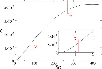
Figure 1: $C$ versus $\bar{\omega}\tau$. Notice the quadratic region extending up to times of order $\tau_{1}$ (inset) and the linear region (20) in the range $\tau_{1}<\tau<\tau_{2}$. The saturation level $2\delta S^{2}\simeq 0.0044$ is in full agreement with (10) [for $N=128$]. We set $x=0.09$ and $m^{2}=5$, so that $\bar{\omega}=2.62$. Observe that $\tau_{2}\simeq 200\;\tau_{1}$ is clearly an intermediate timescale, orders of magnitude smaller than $T_{\rm relax}$. Larger ratios $\tau_{2}/\tau_{1}$ are observed for smaller values of $x$, but the chain of inequalities (IV) always remains valid.

V Diffusion coefficient and intermediate timescales

The presence of the linear region (12) for the correlation function $C$ is observed in the whole range of $x$ investigated. This enables us to define a diffusion coefficient $D$ as the rate at which $C$ increases in its linear regime, so that in the region $\tau_{1}<\tau<\tau_{2}$ we have

$$C=D\tau+C_{0},$$ (20)

where $D$ and $C_{0}$ have in general a nontrivial dependence on $x$. In the following we will perform a systematic study of $D$, which is the physically most relevant quantity and characterizes the Brownian fluctuations. Notice that $C_{0}$ is related to the initial quadratic region (13) and therefore depends on the microscopic details of the motion.

The diffusion coefficient $D$ has no length dimension [$\nu=0$ in (7)] and therefore one expects it to be only a function of $x=g\epsilon=gE/N$ (at fixed $N$ and $m$). This expectation is numerically confirmed with high accuracy. In particular, $D$ is a monotonically increasing function of $x$, as can be seen from Figure 2. Each point in the figure is obtained by averaging at least $5$ numerical solutions with the same value of $x$. For $x\lesssim 0.1$, $D$ is accurately fit by a power law

$$D=\alpha\;x^{\beta},\quad\beta=1.987\pm 0.040.$$ (21)

This is an indication that the intermediate dynamics at these timescales can be tackled by a perturbative approach. Notice that, if one endeavors to fit the curves in Figure 2 with a stretched-exponential law of the type $D\propto\exp({\rm const}\cdot x^{-\delta})$, one finds the very small value $\delta=9.4\cdot 10^{-4}$. In our opinion, this is a rather strong indication in support of a power-law behavior. On the other hand, for large $x$, $D$ saturates to a constant ($m$-independent) value. Observe that the coefficient $\beta$ in (21) does not depend on $m$; the $m$-dependence of $\alpha$ will be analyzed in the following (see Figure 3).

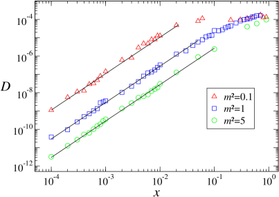
Figure 2: $D$ versus $x=g\epsilon=gE/N$ for different masses. The lines are the power law (21) and the error bars are included in the size of the dots.

The intermediate timescale $\tau_{2}$ is strictly related to the diffusion coefficient $D$, via the saturation value $2\delta S^{2}$ in (10), as discussed in connection with Figure 1. A consistent and natural definition is $\tau_{2}=2\delta S^{2}/D$, so that for $x\lesssim 0.1$

$$\tau_{2}\;\propto\;x^{-\beta}\simeq\;x^{-2}.$$ (22)

Note that in order to measure $\tau_{2}$ it is not even necessary to perform a numerical integration of the Hamilton equations for times of order $\tau_{2}$. It suffices to integrate them up to times larger than $\tau_{1}$ ($\ll\tau_{2}$), get $D$ and hence $\tau_{2}$.

The analytic dependence (22) of $\tau_{2}$ on $x$ is in full agreement with previous results and suggests the validity of a perturbative approach Lepri . One expects that for sufficiently small $x$ a sensible fraction of the phase space is covered with KAM tori, allowing only Arnol’d diffusion and yielding a consistent suppression of diffusion and a rapid divergence of the macroscopic equilibrium time. Related analytical and numerical work hints at a non-analytic divergence (such as a stretched exponential) of the macroscopic timescales (such as $T_{\rm relax}$) Nekhoroshev ; ParisiSFT ; Casetti97 for $x\to 0$. The fact that the intermediate timescale here analyzed diverges with a power law (22) indicates the local presence of a Brownian motion (in the region of parameters studied), so that diffusion should be suppressed on macroscopic regions of phase space.

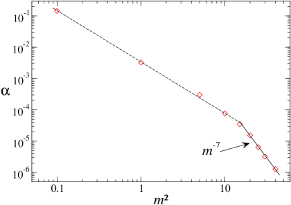
Figure 3: $\alpha=D/x^{2}$ versus $m^{2}$ [in the quadratic region (21)]. The solid line is theoretical prediction for large masses $\alpha\propto m^{-7}$. The dashed line is the fit $\alpha\propto m^{-3.3}$.

The dependence of $\alpha=D/x^{2}$ on $m$ is not trivial. However, in the region of validity of (21) and for large masses $m^{2}\gg 1$, one expects a power-law dependence $\alpha\propto m^{-7}$. Indeed, for large $m^{2}$ we get from (2) $\epsilon\sim m^{2}q^{2}$, so that, at fixed $\epsilon$, $q$ scales like $1/m$. Therefore the strength $g$ of the quartic potential (and hence $x=g\epsilon$) scales like $m^{4}$. Considering that $[D]=t^{-1}$ and the characteristic oscillation time (14) scales like $1/m$, an additional factor $m$ is obtained, yielding

$$\alpha\propto m^{-7},\qquad\mbox{for}\quad m^{2}\gtrsim 15\ .$$ (23)

As shown in Figure 3, this prediction is well confirmed by our numerical data, provided $m^{2}\gtrsim 15$. For $0.1\lesssim m^{2}\lesssim 15$ we numerically found $\alpha\propto m^{-3.3}$, for which we offer no explanation. Moreover, for $m\to 0$ one expects a qualitatively different situation, since $\omega_{\mathrm{MAX}}/\omega_{\mathrm{min}}=\sqrt{4+m^{2}}/m\to\infty$, such a ratio representing the available primary resonances between normal modes Lichtenberg . Actually, we observed the formation of metastable states for $m^{2}\lesssim 0.05$ (not shown in Figure 3): as a consequence, the correlation function showed marked oscillations of definite frequency, hindering a consistent definition of a diffusion coefficient.

VI Conclusions

The analytic (power-law) divergence (22) of the intermediate timescales describing the Brownian motion on the constant energy surface suggests that a perturbative approach, based on a Liouville-Fokker-Planck equation Prigogine60 should apply, at least locally, and that an eventually non-analytic divergence of the relaxation time from far to equilibrium should be ascribed to a nontrivial structure of the phase space at larger scales. The dependence of the intermediate timescale on the mass and the presence of long-lived metastable states indicates that the problem is very involved also at the (supposedly simpler) level of the local dynamics in phase space. In this context, one might speculate that the relaxation from states that are not too far to equilibrium depends on the “mesoscopic” features of phase space. (The expression “mesoscopic” is not used here in its most familiar meaning, related to the interplay of classical and quantum effects, but rather in the sense of intermediate between “microscopic” and “macroscopic,” i.e. pertaining to the total system.) The approach we propose enables one to extract sensible information from the dynamics at intermediate timescales (from close to equilibrium) that are usually less studied than the longer ones, describing the relaxation from far to equilibrium. This has obvious positive spinoffs from the perspective of numerical investigations, as it requires less computing time. From a more conceptual viewpoint, we have proved the existence of a diffusive process (without introducing any randomization “by hand”), that constitutes a building block for the global equilibration process.

*

Appendix A

Let us show that, in order to compute the average of any function of the spectral entropy $S$, the microcanonical and the canonical ensemble are equivalent. This conclusion is a consequence of the following theorem:

In an ensemble of $N$ noninteracting integrable classical systems, where the energies $E_{i}>0$ are homogeneous functions of the action variables $I_{i}$, the average of functions of the kind $F(E_{i}/E)$, where $E=\sum E_{i}$, computed according to the Boltzmann distribution, is equal to that computed according to the microcanonical distribution. Moreover, this average is independent of the temperature $\beta$ of the canonical ensemble and the energy ${\mathcal{E}}$ of the microcanonical ensemble.

We prove this theorem by calculating the canonical average of a quantity $F$ (the angle variables are trivially integrated over since they do not contribute to the energies)

$$\left<F\right>_{c} = \frac{1}{Z_{c}}\int d^{N}\;Ie^{-\beta E}F\left(\frac{E_{i}}{E}\right)$$ (24)

$$= \frac{1}{Z_{c}}\int d^{N}E\;J(E_{i})e^{-\beta E}F\left(\frac{E_{i}}{E}\right),$$

where

$$Z_{c}=\int d^{N}I\;e^{-\beta E}$$ (25)

is the canonical partition function and $J=\|\partial I_{j}/\partial E_{i}\|$ the Jacobian. Due to our hypotheses, this is a homogeneous function of the $E_{i}$’s. We obtain

$$\left<F\right>_{c} = \frac{1}{Z_{c}}\int d^{N}E\int_{0}^{\infty}d\xi$$ (26)

$$\times\delta\left(\xi-\sum_{i}E_{i}\right)e^{-\beta E}J(E_{i})F\left(\frac{E_{i}}{E}\right)$$

$$= \frac{1}{Z_{c}}\int_{0}^{\infty}d\xi\;e^{-\beta\xi}\xi^{N-1}$$

$$\times\int d^{N}x\;J(\xi x_{i})\delta\left(1-\sum_{i}x_{i}\right)F\left(x_{i}\right)$$

$$= \frac{1}{Z_{c}}\int_{0}^{\infty}d\xi\;\xi^{N-1+N\alpha}e^{-\beta\xi}$$

$$\times\int d^{N}xJ(x_{i})\delta\left(1-\sum_{i}x_{i}\right)F\left(x_{i}\right)$$

$$= \frac{1}{Z_{c}}\beta^{-N(1+\alpha)}\Gamma(N(1+\alpha))$$

$$\times\int d^{N}xJ(x_{i})\delta\left(1-\sum_{i}x_{i}\right)F\left(x_{i}\right),$$

where $\Gamma$ is the Gamma function, we defined $x_{i}=E_{i}/\sum_{j}E_{j}$ and used the homogeneity of the Jacobian to write

$$J\left(\xi x_{i}\right)=\xi^{N\alpha}J(x_{i}),$$ (27)

which defines the quantity $\alpha$. By repeating the same derivation with $F=1$, one readily shows that

$$\frac{Z_{c}}{\beta^{-N(1+\alpha)}}=\Gamma(N(1+\alpha))\;\frac{Z_{m}}{{\mathcal{E}}^{N-1+N\alpha}},$$ (28)

where the $Z_{m}$ is the microcanonical partition function

$$Z_{m}=\int d^{N}I\;\delta({\mathcal{E}}-E).$$ (29)

Incidentally, notice that both sides of (28) are independent of $\beta$ and ${\mathcal{E}}$. In conclusion

$$\left<F\right>_{c} = \frac{{\mathcal{E}}^{N-1+N\alpha}}{Z_{m}}\int d^{N}x\;J(x_{i})\delta\left(1-\sum_{i}x_{i}\right)F\left(x_{i}\right)$$ (30)

$$= \frac{1}{Z_{m}}\int d^{N}I\;\delta\left({\mathcal{E}}-E\right)F\left(\frac{E_{i}}{E}\right)=\left<F\right>_{m}.$$

This proves our assertion. Equations (9)-(10) are readily obtained by explicitly calculating the (simpler) canonical average of $F=S$ and $F=S^{2}$.

As a corollary, one sees that if the $E_{i}$s are random variables distributed with $e^{-E_{i}}$, the variables $x_{i}=E_{i}/\sum_{j}E_{j}$ are distributed like $\delta(1-\sum_{j}x_{j})$. This provides a fast numerical recipe to generate microcanonically distributed variables.

References

- (1) E. Fermi, J. Pasta and L. Ulam, Collected Papers of Enrico Fermi, E. Segrè ed., Univ. of Chicago Press, Chicago (USA), 1965, Vol.2, p.978.
- (2) Y. G. Sinai, Sov. Math. Dokl. 4, 1818 (1963).
- (3) A. N. Kolmogorov, Dokl. Akad. Nauk. SSSR 30, 299 (1954); V. I. Arnol’d, Russ. Math. Surv. 18, n.6, 85 (1963); J. Moser, Mem. Am. Math. Soc. 81, 1, (1968).
- (4) N. N. Nekhoroshev, Russ. Math. Surv. 32, 1 (1977). G. Benettin and G. Gallavotti, J. Stat. Phys. 44, 293 (1986).
- (5) V. I. Arnol’d, Sov. Math. Dokl. 5, 581 (1964).
- (6) A. J. Lichtenberg and M. A. Lieberman, Regular and chaotic dynamics, Springer, New York, 1992; J. Guckenheimer and P. Holmes, Nonlinear oscillations, and dynamical systems, Springer, New York, 1997.
- (7) G. Parisi, Statistical Field Theory, Perseus, Reading (Massachussetts, USA), 1998.
- (8) L. Casetti et al., Phys. Rev. E 55, 6566 (1997); M. Pettini and M. Landolfi, Phys. Rev. A 41, 768 (1990); M. Pettini and M. Cerruti-Sola, ibid. 44, 975 (1991); R. Livi et al, ibid. 31, 1039 (1985).
- (9) G. P. Tsironis and S. Aubry, Phys. Rev. Lett. 77 5225 (1996); A. Bikaki et al., Phys. Rev. E 59, 1234 (1999); R. Reigada, A. Sarmiento and K. Lindenberg, Physica A 305, 467 (2002).
- (10) G. Parisi, Europhys. Lett., 40, 357 (1997).
- (11) S. Lepri, Phys. Rev. E 58, 7165 (1998).
- (12) M. Abramovitz and I. A. Stegun, Handbook of Mathematical Functions, Dover, New York, 1968.
- (13) C. G. Goedde, A. J. Lichtenberg and M. A. Lieberman, Physica D 59, 200 (1992).
- (14) B. Mandelbrot, The Fractal Geometry of Nature, Freeman, New York, 1983.
- (15) C. W. Gardiner, Handbook of Stochastic Methods, Springer, Berlin, 1990; N. G. Van Kampen, Stochastic processes in physics and chemistry (Elsevier, Amsterdam 1992).
- (16) I. Prigogine, Non-Equilibrium Statistical Mechanics, Interscience, New York, 1962; R. Balescu, Equilibrium and Non Equilibrium Statistical Mechanics, Wiley, 1991.