Lipids diffusion mechanism of stress relaxation in a bilayer fluid membrane under pressure.

Abstract

A theory of a lateral stress relaxation in a fluid bilayer membrane under a step-like pressure pulse is proposed. It is shown theoretically that transfer of lipid molecules into a strained region may lead to a substantial decrease of the membrane’s free energy due to local relaxation of the stress. Simultaneously, this same effect also causes appearance of the spontaneous curvature of the membrane. Proposed stress relaxation mechanism may explain [1] recent experimental observations of a collapse of the ionic conductance through the protein mechanosensitive channels piercing the E-coli’s membrane [2, 3]. The conductance decreases within seconds after opening of the channels by applied external pressure. The time necessary for a propagation of a stress over the largest membrane’s dimension is $5\div 6$ orders of magnitude shorter. On the other hand, theoretical estimates of the phospholipids diffusion time inside the strained area is favorably comparable with the experimental data [3]. Our theory also predicts that the membrane’s curvature increases simultaneously with the stress relaxation caused by the lipids diffusion. This effect is proposed for experimental check up of the theoretical predictions.

I Introduction

The functioning of the protein channels (pores) in the cell membranes regulates flows of ions in- and out of the cell, thus influencing signal transmission processes in the neural networks of the biological systems [4]. Therefore, the gating mechanisms of the channels are of great interest for the fundamental and practical matters, e.g. like enhancement of the efficiency of the general anesthesia methods [5]. Mechanical stresses in cell membranes may cause opening of the protein mechanosensitive (MS) channels [6], which hence play a role of mechanoreceptors in the cellular organisms. One of the biological objects convenient for experimental study is the large conductance MS channel (MscL) in the inner membrane of the Escherichia coli (E-coli) bacteria. It is possible to measure a single channel conductance, an find its dependence on the internal lateral tension in the membrane. The tension, which causes opening of the channel, could be evaluated using video microscopy measurements of the membrane curvature formed under the applied external pressure [2].

The time-dependence of the membrane’s conductance observed by C.C. Hase et al. [3] reveals gradual collapse of the ionic currents through the MscL’s within seconds after their opening. According to existing hypothesis [1], this may happen due to mutual slide of the lipid monolayers, constituting a bilayer membrane of the E-coli. This slide would then encourage a relaxation of the lateral stress inside the membrane, which is necessary for an opening of the MscL’s. The slide of the monolayers should be encouraged by the same pressure pulse, which causes initial opening of the ionic channels.

In this paper we propose a theory of such a stress-relaxation process and demonstrate that the slide of the monolayers under a constant external pressure is indeed thermodynamically advantageous. In order to show this, we calculate the free energy difference between two possible equilibrium states of a membrane under a pressure gradient pulse.

The first (”intermediate”) equilibrium state, is achievable shortly after the beginning of a pressure pulse $P$, within the time of propagation of the mechanical stress along a membrane $\Delta t>10^{-6}$sec (evaluated below). In this state the initial numbers of the phospholipid molecules in the monolayers constituting the bilayer membrane, $N_{1}$ and $N_{2}$, yet, remain unchanged: $N_{1}=N_{2}=N_{0}$. Here $N_{0}$ is the number of the molecules in a monolayer before external pressure gradient is applied. We neglect a small probability [7, 8] of the flip-flop process, i.e. exchange of lipids between the monolayers. Then, the tensions $T_{1}$, $T_{2}$, in both monolayers approximately coincide, since the radius $R$, of the membrane is of order $1\div 2\mu m$, while its thickness $l_{0}$, is about $2nm$ [3].

In the second, (final) equilibrium state, achievable within diffusion time $\tau\sim 1\mbox{sec}\gg\Delta t$, the extra lipid molecules from the outer patch of E-coli’s material have enough time to be ”sucked in” inside the concave-side monolayer, see Fig. 1, until the tension in the monolayer is relaxed at a finite curvature: $T_{1}=0$. Then, the tension $T_{2}$ in the convex-side monolayer (which is stuck to the pipette and thus can not absorb extra molecules [2, 3], see Fig. 1) alone maintains a mechanical equilibrium under the same external pressure difference $P$ across the membrane. In accord with the Laplace’s law we have:

$$T_{1}+T_{2}=T_{2}=Pr/2;\;\;\;\mbox{at}\;\;T_{1}=0.$$ (1)

Here $r$ is the radius of curvature. Next, we calculate self-consistently the free energy of the whole system: membrane+patch, in both equilibrium states. Important, the free energy in the relaxed, second state, proves to be lower than in the intermediate state with constrained numbers of lipids, Fig. 2. Choosing the second, relaxed state we then evaluate the number $\Delta N_{1}$ of the ”sucked in” lipids and find, see Fig. 4, that it is of a macroscopic magnitude, e.g. $\Delta N_{1}\sim 15{\%}N_{1}$. Based on these results and using experimentally determined diffusion coefficient of individual lipid molecules in bio-membranes at room temperature [9] $D\sim 1\div 20\mu m^{2}/sec$, we estimate the characteristic diffusion time $\tau$:

$$\tau\sim\displaystyle\frac{\Delta N_{1}}{N_{1}}\frac{R^{2}}{D}\sim 1\mbox{sec},$$ (2)

which is comparable by the order of magnitude with the experimental data [3]. Thus, we predict a macroscopic increase of the number of lipid molecules $\Delta N_{1}$ in the concave monolayer and, hence, propose to measure the concomitant change of the weight of the part of the membrane sucked in in the pipette during the decrease of the ionic conductance (in the setup of the works [2, 3]).

Besides, as it is apparent from Fig. 2, the equilibrium curvature of the membrane (indicated with the arrows) also changes significantly as the membrane passes from the intermediate to the final equilibrium state. Hence, it should be possible to check our theory also by measuring the time-dependent increase of the curvature, which should then accompany the decay of the ionic conductance observed [3] under a constant external pressure gradient.

The plan of the article is as follows. In Section II we describe a free energy functional in our model of a bilayer membrane and derive the self-consistent equations for the membrane in the equilibrium state under a constant pressure gradient. Both versions of the equilibrium state discussed above are considered. In Section III we give analytical and numerical solutions of the derived equations and discuss in detail corresponding calculated dependencies. Finally, we discuss in the last Section IV possible experimental verifications and future improvements of the theory.

II The model free energy

We use the microscopic model of a bilayer membrane as described e.g. in [7, 8]. First write a single i-th monolayer ($i=1,2$) free energy per lipid molecule $f_{i}$:

$$f_{i}=f_{si}+f_{hi}+f_{ti}\equiv\gamma a_{i}+\frac{C}{a_{i}}+\displaystyle\frac{k_{s}}{2}(l_{i}-l_{s})^{2}$$ (3)

Here $f_{si}$ is the external surface energy of the monolayer, which increases with the area per lipid molecule $a_{i}$ due to the hydrocarbon tails interaction energy with the solvent. The short-range repulsion between the polar molecular heads at the surface of the membrane is represented by the second term in Eq. (3). The third term, though looks like a spring elastic energy (with not stretched spring length $l_{s}$), codes for the entropic repulsion between the hydrocarbon tails in the depth of each monolayer [8]. In what follows we omit the second term in Eq.(3) on the empirical grounds [8] relevant for the chain molecules in phospholipid bilayers. There is no interface energy term included in (3) for the internal surfaces of the monolayers forming the bilayer, as the latter are not reachable for the solvent molecules. We also assume a vanishing interdigitation of the tails between the adjoint monolayers. The length of a lipid molecule $l_{i}$, i.e. the thickness of the i-th monolayer, is not an independent variable from the aria per molecule $a_{i}$. The volume $v$ per lipid molecule is conserved, i.e. the latter could be considered as incompressible [7, 8]. Due to this conservation condition the length $l_{i}$ is related to the mean and gaussian curvatures $H$ and $K$ at the interface between the monolayers by a well known differential geometry formulas [7]:

$$l_{1}=l_{01}-l_{01}^{2}H+\displaystyle\frac{2}{3}l_{01}^{3}K$$ (4)

$$l_{2}=l_{02}+l_{02}^{2}H+\displaystyle\frac{2}{3}l_{02}^{3}K$$ (5)

Here the change of sign in front of $H$-term in the equation (5) relative to that in equation (4) is due to a simple geometrical fact that the external normal vector to e.g. the layer 1 is simultaneously an internal normal vector to the layer 2 at their mutual interface. Different $l_{0i}$ parameters just reflect the incompressibility of the lipid molecules mentioned above:

$$l_{0i}=\frac{v}{a_{i}}$$ (6)

Substituting Eqs. (4),(5) into the third term of Eq. (3) one finds contributions to the free enrgy from the tails in the form:

$$f_{t1}=\frac{k_{s}l_{01}^{4}}{2}\left[(H-C_{01})^{2}+\frac{4}{3}C_{01}l_{01}K\right]$$ (7)

$$f_{t2}=\frac{k_{s}l_{02}^{4}}{2}\left[(H+C_{02})^{2}+\frac{4}{3}C_{02}l_{02}K\right]$$ (8)

where parameters $C_{0i}$ have meaning of the local spontaneous curvatures of the $i$-th layer:

$$C_{0i}=\frac{l_{0i}-l_{s}}{l_{0i}^{2}}$$ (9)

We readily recognize the Helfrisch’s formula [10] for the free energy of a membrane in Eqs. (7), (8). In a symmetric bilayer case $N_{1}=N_{2}$ (where again $N_{1}$ and $N_{2}$ signify the numbers of lipid molecules in the 1-st and 2-nd monolayer respectively), with equivalent conditions on the opposite surfaces of the membrane $a_{1}=a_{2}$, the linear in $H$ terms in Eqs. (7), (8) would cancel in the total free energy $F$:

$$F=\sum_{i=1,2}F_{i}=\sum_{i=1,2}N_{i}f_{i}$$ (10)

Nevertheless, as shown below, a linear in $H$ term may arise when the up vs down symmetry of a membrane is broken, e.g. by applied pressure gradient in combination with the different boundary conditions at the monolayers peripheries, see Fig. 1.

To make the whole idea transparent we restrict our present derivation to the case of a spherically ”homogeneous distributions” of molecules, i.e. considering $a_{i}$’s as being different for the different indices i’s, but position-independent within i-th monolayer. Below, we neglect the inhomogeneous distribution of the strain across the thickness of each monolayer. Also, we consider only spherical shapes of the deformed bilayer membrane, while introducing position independent (over the membrane’s surface) mean and gaussian curvatures:

$$H=\frac{1}{r}\,;\;\;\;K=H^{2}=\displaystyle\frac{1}{r^{2}}$$ (11)

where $r$ is the radius of curvature. The radius of the base of the curved membrane is fixed at $R\leq r$, in accord with the fixed radius of the pipette, which sucks in the membrane, and creates a pressure difference $P$ between inside and outside surfaces of the membrane in the experimental setup [2, 3]. According to experimental data [2, 3] the membrane under consideration is rather thin:

$$l_{s}\sim 10^{-3}R\ll R\leq r\,.$$ (12)

Choose direction ”up” inside the pipette, perpendicular to the plane of the initially flat membrane. Also, ascribe indices ”1” and ”2” to the parameters of the lower and upper monolayer of the membrane respectively. Then, the external surface areas $S_{1}$ and $S_{2}$ of the lower (concave) and upper (convex) monolayers and the numbers of the molecules in them are related by the following equations:

$$S_{1}=2\pi(r-l_{1})^{2}\left(1-\displaystyle\sqrt{1-\frac{R^{2}}{(r-l_{1})^{2}}}\right)=N_{1}a_{1}\;;$$ (13)

$$S_{2}=2\pi(r+l_{2})^{2}\left(1-\displaystyle\sqrt{1-\frac{R^{2}}{(r+l_{2})^{2}}}\right)=N_{2}a_{2}\;;$$ (14)

$$\pi R^{2}=N_{0}a_{0}\;,\mbox{at $r=\infty$}.$$ (15)

Here the thicknesses $l_{i=1,2}$ of the i-th monolayer are defined in Eqs. (4), (5). A flat, undeformed membrane has a monolayer thickness $l_{0}=v/a_{0}$ under zero external pressure gradient, where the area per molecule $a_{0}$ is determined from the condition of the minimum of the free energy $F$ defined in Eq. (10):

$$\displaystyle\frac{\delta F}{\delta a_{0}}=0\;,\;\;\;\mbox{at:}\;\;\;a_{1}=a_{2}=a_{0},\;\;\;H=K=0,\;\;\;N_{1}=N_{2}=N_{0}.$$ (16)

Allowing for the experimental setup [1], it is reasonable to suppose that the number of molecules in the upper monolayer $N_{2}$, which ”sticks” by its peripheral to the pipette walls, is fixed during the experiment:

$$N_{2}=N_{0}.$$ (17)

Hence, Eq. (17) together with Eqs. (14), (11), (5), and (6) relates curvature radius $r$ to the area per molecule $a_{2}$:

$$a_{2}=a_{2}(H)$$ (18)

In order to find the equilibrium areas $a_{1}$ and $a_{2}$ one has to solve different sets of self-consistency equations, depending on the conservation/nonconservation of the number of molecules $N_{1}$ in the 1-st monolayer.

When $N_{1}$ is conserved we have:

$$N_{1}=N_{0}=N_{2}.$$ (19)

This equation, together with Eqs. (13), (11), (4), and (6) relates $a_{1}$ to the curvature $H$ similar to Eq. (18):

$$a_{1}=a_{1}(H)$$ (20)

Hence, the only independent variables left are the curvature radius $r$, and the pressure difference across e.g. 1-st monolayer $P_{1}$. The equilibrium values of these parameters minimize the free energy in the equilibrium state of the membrane exposed to the total applied pressure difference $P$:

$$\displaystyle\frac{\delta F_{i}}{\delta a_{i}}=T_{i}=\frac{P_{i}r}{2};\;\;P_{1}+P_{2}=P;\;\;\;P_{1}\approx P_{2}=\frac{P}{2}.$$ (21)

Here the tensions $T_{i}$ (force per unit length of the peripheral) acting in the monolayers are related to the corresponding pressure differences $P_{i}$ via the Laplace’s law (1). A distribution of the pressure differences $P_{i}$, acting across each monolayer, generally should be determined self-consistently by a minimization of the membrane’s free energy $F$, but for a thin membrane (see (12)) we choose them approximately equal.

In the case, when $N_{1}$ is not fixed and the 1-st monolayer is free to absorb extra lipid molecules from the patch/reservoir through its peripheral edge, we substitute equilibrium conditions (21) by the different ones:

$$\displaystyle\frac{\delta\tilde{F}}{\delta a_{1}}=T_{1}=0\;;$$ (22)

$$\displaystyle\frac{\delta\tilde{F}}{\delta a_{2}}=T_{2}=\frac{Pr}{2}\;;$$ (23)

$$\tilde{F}=F+F_{\mbox{patch}}\;,\;\;\;\;N_{1}+N_{2}+N_{\mbox{patch}}=const$$ (24)

where for simplicity the patch free energy $F_{\mbox{patch}}$ is assumed to be equal to the energy of a flat piece of the bilayer membrane under zero pressure and zero tension, which contains $N_{\mbox{patch}}$ lipid molecules in total:

$$F_{\mbox{patch}}=\sum_{i=1,2}\displaystyle\frac{1}{2}{N_{\mbox{patch}}}f_{0};\;\;f_{0}=f_{1}=f_{2}\;\;\mbox{at:}\;\;\;a_{1}=a_{2}=a_{0},\;\;\;H=K=0.$$ (25)

The free energies $f_{i}$ are defined in (3). Finally, we solve equations (21) and (22), (23). As a result, we determine the final state with the lowest energy by a direct comparison of the values of the free energy $\tilde{F}$ in the two different cases of the ”patch-disconnected” and ”patch-connected” membrane.

III Solutions

It is convenient for calculational purposes to rewrite expressions obtained in the previous Section using dimensionless parameters instead of $a_{i}$ and $H$. Because the expressions for the free energy (10), (25) will be studied mainly numerically, we shall incorporate tensions $T_{i}$ into the free energy and look for the minima of the latter on the proper manyfold of the independent variables, rather than solve directly equations (21) - (23) of the Euler-Lagrange type. For this purpose we pass from the free energies $f_{i}$ to the new ones $\tilde{f}_{i}$, which are Helmholtz free energies per lipid molecule in the i-th monolayer under an external pressure difference $P_{i}$:

$$\tilde{f}_{i}=f_{i}(z_{i}(h),h)-\displaystyle\int^{z_{i}(h)}_{z_{0}}\frac{P_{i}v}{2h_{i}(z^{\prime})}dz^{\prime}\;;$$ (26)

$$f_{1}(z_{1},h)\equiv\epsilon_{s}z_{1}+\epsilon_{t}\left\{\displaystyle\frac{h^{2}}{3}(7z_{1}^{-4}-4z_{1}^{-3})+2h(z_{1}^{-2}-z_{1}^{-3})+1+z_{1}^{-2}-2z_{1}^{-1}\right\};$$ (27)

$$f_{0}=f_{1}(z_{0},h=0)=\epsilon_{s}z_{0}+\epsilon_{t}\{1+z_{0}^{-2}-2z_{0}^{-1}\};$$ (28)

$$f_{2}(z_{2},h)=f_{1}(z_{2},-h).$$ (29)

Here dimensionless parameters $z_{i}$ and $h$, as well as the other ones, are defined as follows:

$$\displaystyle z_{i}=\frac{a_{i}l_{s}}{v};\;\;h=\frac{l_{s}}{r}\equiv Hl_{s};\;\;h_{0}=\frac{l_{s}}{R};\;\;\epsilon_{s}=\frac{\gamma v}{l_{s}};\;\;\epsilon_{t}=\frac{k_{s}l_{s}^{2}}{2}.$$ (30)

A dependence $h_{i}(z)$ on the right-hand-side of Eq. (26) is just the inverse of either Eq. (20) or Eq. (18) written in the dimensionless units (30). It is useful for the comprehension of the rest of the paper to mention here orders of magnitude of the main parameters. As it follows from (12): $h\sim 10^{-3}\ll 1$. Next, it follows from the definition (6) and Eqs. (4), (5) that $v\approx l_{s}a_{i}$, which leads to an estimate: $z_{i}\sim 1$. The entropic nature of the $f_{ti}$ term in Eq. (3) is reflected in the temperature dependent coefficient $k_{s}$, which for the known phospholipid bilayers is of the order [8]: $k_{s}l_{s}^{2}\sim 1\div 10kT$, where $k$ is the Boltzman’s constant and $T$ is the absolute temperature. The scale of the surface term $f_{si}$ in Eq. (3) is characterized by the coefficient $\gamma$, which at room temperature is of the order [8]: $\gamma\sim 0.1kT/\AA^{2}$. Gathering all the estimates, and also taking into account that the typical value of an area per molecule is [8]: $a_{i}\sim 60\AA^{2}$, we obtain the following list of the estimates (taken for the room temperature $T\sim 300K$):

$$\displaystyle z_{i}\sim 1;\;\;h\sim 10^{-3};\;\;\epsilon_{s}\sim 10^{-13}\mbox{erg};\;\;\epsilon_{t}\sim 1\div 10\epsilon_{s}.$$ (31)

An additional important dimensionless parameter relates characteristic experimental value of the pressure difference $P\sim 50$mm Hg [2, 3] with the ”microscopical bending energy” $\epsilon_{t}$:

$$\displaystyle\frac{Pv}{2\epsilon_{t}}\sim 4\cdot 10^{-4}\;\;\;\mbox{at:}\;\;\epsilon_{t}\sim 10^{-13}\mbox{erg};\;\;v\sim 1.2\cdot 10^{3}\AA^{3},$$ (32)

where we use an estimate $l_{s}\sim 20\AA$ for the typical length of a phospholipid molecule in a bilayer membrane [8].

Now, coming to a description of the results, we first solve equation for $z_{0}$:

$$\displaystyle\frac{\partial{f_{0}}}{\partial{z_{0}}}=\epsilon_{s}+2\epsilon_{t}\{z_{0}^{-2}-z_{0}^{-3}\}=0$$ (33)

or in the Cardano’s form:

$$z_{0}^{3}+pz_{0}+q=0;\;\;\mbox{where:}\;\;\displaystyle p=-q=\frac{2\epsilon_{t}}{\epsilon_{s}}$$ (34)

$$\mbox{and:}\;\;\displaystyle\left(\frac{q}{2}\right)^{2}+\left(\frac{p}{3}\right)^{3}\equiv\left(\frac{\epsilon_{t}}{\epsilon_{s}}\right)^{2}+\left(\frac{2\epsilon_{t}}{3\epsilon_{s}}\right)^{3}>0.$$ (35)

The inequality in (35) proves that there is a unique real root of the cubic equation (34). In the limit $p\gg 1$ the real root of Eq. (34), first order accurate in $p^{-1}$, is:

$$z_{0}\approx 1-\frac{1}{p}=1-\displaystyle\frac{\epsilon_{s}}{2\epsilon_{t}}.$$ (36)

A Patch-disconnected case

In the patch-disconnected case, or during a short enough time $t$: $\Delta t\leq t\ll\tau$, after an application of a pressure difference $P$ across the membrane’s plane, the numbers of the lipid molecules in the both monolayers of the bilayer membrane remain equal: $N_{1}=N_{2}=N_{0}$. Hence, the areas per molecule $a_{i=1,2}$ also remain equal to each other, while simultaneously undergoing an increment with respect to the initial undeformed value $a_{0}=vz_{0}/l_{s}$. Neglecting small corrections $\propto l_{i}/r\sim 10^{-3}$ in Eqs. (13), (14) one finds:

$$z_{i}(h)\approx z_{0}\frac{2h_{0}^{2}}{h^{2}}\left(1-\displaystyle\sqrt{1-\frac{h^{2}}{h_{0}^{2}}}\right);\;\;i=1,2.$$ (37)

Thus, $a_{i}$ ranges from $a_{0}$ to $2a_{0}$, or equivalently: $z_{0}\leq z_{i}(h)\leq 2z_{0}$, on the interval of the membrane’s curvatures: $0\leq 1/r\leq 1/R$, or in dimensionless units: $0\leq h\leq h_{0}$. The inverse of Eq. (37) yields:

$$h(z_{i})\approx\frac{2h_{0}z_{0}}{z_{i}}\displaystyle\sqrt{\frac{z_{i}}{z_{0}}-1};\;\;i=1,2.$$ (38)

Now, we substitute (38) into the integral on the right-hand-side of (26) and find after an integration:

$$\tilde{f}_{i}=f_{i}(z_{i}(h),h)-\displaystyle\frac{P_{i}vz_{0}}{2h_{0}}\sqrt{\frac{z_{i}(h)}{z_{0}}-1}\left[1+\frac{1}{3}\left(\frac{z_{i}(h)}{z_{0}}-1\right)\right].$$ (39)

Substituting $P_{i}=P/2$ in (39), and then substituting $\tilde{f}_{i}$ from Eq. (39) into Eq. (10) instead of $f_{i}$ we find the $F(h)/N_{0}$ dependence (in the units of $\epsilon_{t}$) plotted with the dashed curve in Fig. 2. A position of the minimum, defined as the point at which $\partial F/\partial h$ changes sign, is indicated with the vertical arrow. It is apparent from the Fig. 2 that the minimum is rather shallow and happens at the curvature radius $r$ comparable with the radius $R$ of the pipette (e.g. of the membrane’s base). This indicates a substantial deviation of the membrane from the planar shape and is in accord with the experiments demonstrating nearly spherical shape of the membrane at this pressure [2, 3]. Thus, it is not surprising that, unlike in the case of a weakly bent thin plate [11], now both sides of the membrane’s surface are stretched. Hence, an important property of this deformed state is the presence in both monolayers of nearly equal tensions $T_{i}$ stretching the membrane and causing opening of the protein mechanosensitive channels [2, 3]: $T_{1}\approx T_{2}=Pr/4$. Let us consider another situation, where the symmetry of the tension distribution is broken.

B Patch-connected case

Now assume that enough time had elapsed after the beginning of the pressure pulse for a transfer of a substantial amount of the lipid molecules from the patch to the ”sucked in the pipette” part of the membrane (see Fig. 1): $t\geq\tau$. Hence, we consider the number of molecules $N_{1}$ in the patch-connected monolayer as an additional variational parameter. In this case the system of equations (22), (23) applies. The first equation written in the dimensionless variables and allowing for the general expression (27) yields:

$$\epsilon_{s}+\epsilon_{t}\displaystyle\left\{\displaystyle\frac{h^{2}}{3}\left(-\frac{28}{z_{1}^{5}}+\frac{12}{z_{1}^{4}}\right)+2h\left(\frac{3}{z_{1}^{4}}-\frac{2}{z_{1}^{3}}\right)+2\left(\frac{1}{z_{1}^{2}}-\frac{1}{z_{1}^{3}}\right)\right\}=0.$$ (40)

This equation defines now a $z_{1}(h)$ for the tension-free monolayer with a finite curvature $h\neq 0$, and thus, substitutes equation (33), which is valid for the tension-free, but flat case ($h=0$). Simultaneously, equation (37) remains valid for the 2-nd monolayer with conserved number of lipids $N_{2}=N_{0}$, and provides dependence $z_{2}(h)$:

$$z_{2}(h)\approx z_{0}\frac{2h_{0}^{2}}{h^{2}}\left(1-\displaystyle\sqrt{1-\frac{h^{2}}{h_{0}^{2}}}\right).$$ (41)

In the Fig. 3 we present our numerical solutions of the Eqs. (33) (dash-dotted curve) , (40) (solid curves), as well as a dependence given by Eq. (41) (dotted curve). The insert in Fig. 3 demonstrates that actually $z_{1}(h)$ remains nearly equal to $z_{0}$ at all curvatures $h$. This result is not surprising. Namely, equations (33) and (40) differ only by $\propto h^{2}\ll 1$ and $\propto h\ll 1$ terms. This means, that the tension-free, relaxed 1-st monolayer, in order to reach its final equilibrium state, absorbs as much molecules from the patch as necessary to compensate for an increase of its area at a finite curvature. In this way the area per molecule remains nearly constant and equal to $\approx z_{0}$ (see insert in Fig. 3). Then, as in the flat case, the equilibrium value $z_{1}$ is again determined by the balance of the surface tension and entropic repulsion of the lipid tails. Using dimensionless area $z_{1}(h)$ determined from (40), we find the (variable) number of the lipid molecules $N_{1}(h)$, normalized by $N_{0}$, as a function of curvature $h$, see Fig. 4. This result was obtained using the following formula:

$$\displaystyle\frac{N_{1}}{N_{0}}=\displaystyle 2\frac{z_{0}}{z_{1}(h)}\left(\frac{h_{0}}{h}\right)^{2}\left(1-\sqrt{1-\left(\frac{h}{h_{0}}\right)^{2}}\right),$$ (42)

where equation (13) and definitions (30) where used.

Now, in order to find the equilibrium value of the curvature $h$ (indicated with the arrow in Figs. (3),(4)) at a given pressure difference $P$, we calculate the total free energy $\tilde{F}$ from Eq. (24) normalized by $N_{0}$ using the following expression:

$$\frac{\tilde{F}}{N_{0}}=f_{1}(z_{1}(h),h)\frac{N_{1}}{N_{0}}+f_{2}(z_{2}(h),h)-\displaystyle\frac{Pvz_{0}}{2h_{0}}\sqrt{\frac{z_{2}(h)}{z_{0}}-1}\left[1+\frac{1}{3}\left(\frac{z_{i}(h)}{z_{0}}-1\right)\right]-$$ (43)

$$\displaystyle f_{0}\left(\frac{N_{1}}{N_{0}}-1\right).$$ (44)

The physical meaning of the factor $N_{1}/N_{0}$ in front of $f_{1}$ in combination with the last subtracted term $\propto f_{0}$ in (44) is simple. Namely, the total number of molecules in the system membrane$+$patch is conserved. Therefore, an increase of the number of molecules in the first monolayer, with the free energy per molecule $f_{1}$, occurs at expense of the decrease of the number of molecules in the patch, with the energy per molecule $f_{0}$. Calculation of the free energy ${\tilde{F}}/{N_{0}}$, normalized by $\epsilon_{t}$, provides its dependence on $h$ expressed with the solid curve in Fig. 2. The arrow indicates position of the minimum of the free energy (obtained from the calculation of the zero root of the first derivative of the free energy with respect to the curvature).

We have also calculated the dependencies of the dimensionless equilibrium curvature $h=R/r$ on the applied pressure difference $P$ for the symmetric strain (dashed line): $T_{1}=T_{2}$, and asymmetric strain (solid line): $T_{1}=0,T_{2}\neq 0$, equilibrium states, see Fig. 5. As it follows from the figure, the power-law dependencies prove to be the same: $1/r\sim const\cdot P^{\alpha},\;\alpha\approx 1/3$, but with the constant pre-factor slightly smaller in the symmetric case.

The influence of the effective surface tension energy $f_{si}=\gamma a_{i}$ in Eq. (3), characterized by the energy $\epsilon_{s}$ (30), is demonstrated in Fig. 6. Here, it is obvious, that an increase of the surface energy coefficient at a fixed entropic repulsion $\epsilon_{t}$, causes a greater bending rigidity of the membrane and as a result, a decrease of the equilibrium curvature caused by an applied external pressure difference.

IV Conclusions and experimental proposals

A direct comparison of the two curves in Fig. 2 leads to the main conclusion of this work, i.e. the free energy of the relaxed, partially tension-free asymmetric equilibrium state: $T_{1}=0,T_{2}=Pr/2$ is lower than the free energy of the non-relaxed symmetric equilibrium state: $T_{1}\approx T_{2}=Pr/4$. Thus, the membrane would change its state until the equilibrium state with the lowest free energy would be reached. The number of the lipids in the 1-st monolayer $N_{1}$ in the relaxed state is greater than the initial one $N_{0}$ by a macroscopical amount ($\sim 15\%N_{0}$, see Fig. 4). Hence, a process of reaching the relaxed state would take time necessary for diffusion of the molecules from the patch into the 1-st monolayer through its peripheral edge (see Fig 1). This time, $\tau$, as evaluated in Section II, Eq. (2), is of order of seconds, and thus is in correspondence with the characteristic time of the collapse of the ionic conductance through the protein mechanosensitive channels piercing the E-coli’s membrane [3]. Hence, our theory confirms the idea [1], that an inter-layer slide in a membrane, soon after the beginning of the pressure pulse, may cause a relaxation of the lateral stress. This stress had initially opened the protein mechanosensitive channels and thus had given rise to the ionic conductance. Closing back of the channels within seconds after the beginning of the pulse would cause simultaneous decrease of the ionic conductance as seen experimentally [3]. A separate consideration of the two equilibrium states discussed above, is justified by the fact that the characteristic stress relaxation time: $\tau\sim 1sec$ differs by 5$\div$6 orders of magnitude from the characteristic time $\Delta t$ necessary for a propagation of the bending deformations over a membrane with the linear dimensions $R\sim 1\mu m$:

$$\displaystyle\Delta t\sim R^{2}\left(\frac{\rho l_{0}}{\epsilon_{t}}\right)^{1/2}\sim 10^{-8}cm^{2}\left(\frac{1g/cm^{3}\cdot 10^{-7}cm}{10^{-13}erg}\right)^{1/2}\sim 10^{-5}sec\;,$$ (45)

where we used a well known formula for the frequency of the bending waves in a thin plate [11]:

$\displaystyle\omega=q^{2}\left(\frac{k_{B}}{\rho l_{0}}\right)^{1/2},$

where $k_{B}$ is a bending modulus, $\rho$ is a mass density, $l_{0}$ is a thickness, and $q$ is a wave-vector. We also allowed for the role of a bending coefficient $k_{B}$ played by the energy $\epsilon_{t}$, which follows from direct comparison of the free energy expressions (7), (8) and the definition of $\epsilon_{t}$ given in (30).

Based on our results, shown in Figs. 2, 4, we propose here the following possible experimental verifications of the theory. First, it is obvious from the Fig. 2 that the equilibrium curvature is greater in the relaxed state than in the non-relaxed one, changing correspondingly from $1/r=0.525R^{-1}$ in the ”intermediate” equilibrium state to $0.675R^{-1}$ in the relaxed state. Hence, we propose to measure this change experimentally as an accompanying process of the decrease of the ionic conductance. This change of curvature signifies a simple fact. Shortly after the application of the pressure difference $P$ it is balanced by the two strained monolayers of a membrane. After enough time has elapsed, a relaxation of the strain in the 1-st monolayer occurs, and hence, only the strain in the 2-nd monolayer compensates the applied pressure, thus the curvature has to change.

Second, from Fig. 4 it follows that, as a result of the relaxation of the strain in the 1-st monolayer, this monolayer acquires extra lipid molecules from the patch, hence the number of molecules in the pipette increases by: ($\Delta N_{1}\approx 15\%N_{0}$). As this change $\Delta N_{1}$ is macroscopic, a corresponding increase of the weight of the sucked in membrane during, the decrease of the ionic conductance should be, in principle, measurable.

Finally, we mention some possible future improvements of the theory. These could be made by lifting of our simplifying restrictions of the homogeneity of the lateral stresses (tensions) across the thickness of each monolayer, as well as the approximation of a constant area per molecule over each external surface of the membrane. As a consequence, in a more complete scheme of derivations one would like not to restrict himself to the spherical symmetry of the membrane’s shape. Nevertheless, we believe that these improvements can not overturn the main physical concept considered in this paper of a diffusion mechanism of a stress relaxation in a bilayer membrane with an inter-layer slide.

V Figure Captions

Fig. 1. Sketch of the experimental setup [2]. The numbering 1,2 of the monolayers within a bilayer membrane is indicated.

Fig. 2. Free energy $F/{(\epsilon_{t}N_{0})}$ normalized by $\epsilon_{t}$ and number of lipid molecules $N_{0}$ versus dimensionless curvature $h$. Solid curve corresponds to the asymmetric strain state with $N_{2}=N_{0}<N_{1}$. Dashed curve corresponds to the symmetric strain case with conserved numbers of lipids in the monolayers: $N_{1}=N_{2}=N_{0}$. Arrows indicate positions of the minima of the free energy.

Fig. 3. Dimensionless areas per molecule $z_{i}$ in the i-th monolayer of a bilayer membrane as functions of the membrane’s curvature $h$ in the asymmetric strain state $T_{1}=0,T_{2}=Pr/2$ (see text). Arrow indicates equilibrium value of the curvature. $z_{0}$ is the equilibrium value under zero external pressure difference.

Fig. 4. Calculated number of the lipid molecules $N_{1}$ in the first monolayer as a function of curvature $h$ in the asymmetric strain state $T_{1}=0,T_{2}=Pr/2$. Arrow indicates equilibrium value of the curvature at $Pv/(2\epsilon_{t})=0.0004$.

Fig. 5. Calculated dependencies of the dimensionless equilibrium curvature $h=R/r$ on the applied pressure difference $P$ for the symmetric strain (dashed line) and asymmetric strain (solid line) equilibrium states in the logarithmic scales.

Fig. 6. Free energy $F/{(\epsilon_{t}N_{0})}$ normalized by $\epsilon_{t}$ and number of lipid molecules $N_{0}$ versus dimensionless curvature $h$. All notations are as in Fig. 2. The main panel corresponds to the ratio $\epsilon_{t}/\epsilon_{s}=50$, which is 10 times greater than for the Fig. 2. An insert calculated for the ratio $\epsilon_{t}/\epsilon_{s}=0.05$. Arrows indicate equilibrium values of the curvature.

 

FIG. 1.:

 

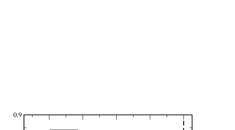
FIG. 2.:

 

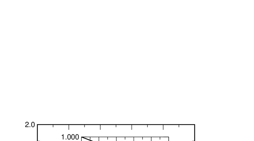
FIG. 3.:

 

FIG. 4.:

 

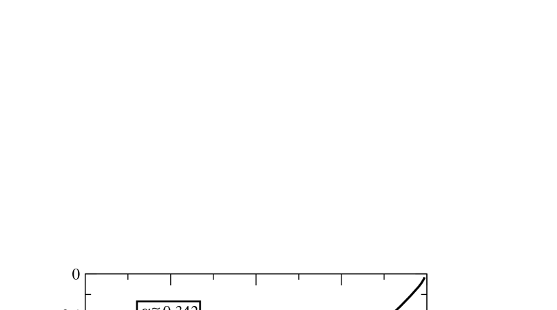
FIG. 5.:

 

FIG. 6.:

REFERENCES

- [1] S.I. Sukharev, private communication.
- [2] S.I. Sukharev, W.J. Sigurdson, C. Kung, and F. Sachs, J.Gen.Physiol. 113, 525 (1999).
- [3] C.C. Hase, A.C. Le Dain, and B. Martinac, J. Biol. Chem. 270, 18329 (1995).
- [4] Ming Zhou, J.H. Morais-Cabral, S. Mann, and R. MacKinnon, Nature 411, 657 (2001); D.A. Doyle, J.M. Cabral, R.A. Pfuetzner, A. Kuo, J.M. Gulbis, S.L. Cohen, B.T. Cahit, and R. MacKinnon, Science, 280, 69 (1998).
- [5] R.S. Cantor, Biophysical Journal 76, 2625 (1999).
- [6] S. Sukharev, M. Betanzos, C.-S. Chiang, and H.R. Guy, Nature 409, 720 (2001).
- [7] S.A. Safran, ”Statistical thermodynamics of surfaces, interfaces and membranes”(Frontiers in Physics, vol.90), 270 p., Perseus Pr. Publisher, 1994.
- [8] A. Ben-Shaul, Molecular theory of chain packing, elasticity and lipid-protein interaction in lipid bilayers. In: Dynamics of Membranes. Elsevier/North Holland, Amsterdam, pp.359-401, 1995; T.-X. Xiang and B.D. Anderson, Biophysical Journal 66, 561 (1994).
- [9] A. Sonnleitner, G.J. Schúltz, and Th. Schmidt, Biophysical Journal 77, 2638 (1999).
- [10] Ou-Yang Zhong-Can and W. Helfrich, Phys. Rev. Lett. 59, 2486 (1987); and Phys. Rev. A 39, 5280 (1989);and Hu Jian-Guo and Ou-Yang Zhong-Can, Phys. Rev. E 47, 461 (1993); and Q.H. Liu, H.J. Zhou, J.X. Liu, and O.Y. Zhong-Can, Phys. Rev. E 60, 3227 (1999).
- [11] L.D. Landau and E.M. Lifshitz, ”Theoretical Physics”, Vol. 7 ”Theory of Elasticity”, Pergamon Press, N.Y., 1980.