Theory of superconducting fluctuations in the thinest carbon nanotubes

Abstract

The low-energy electronic Hamiltonian for the thinest zigzag carbon nanotube, embedded into a dielectric host, is derived and its phase diagram is discussed. The specific multi-band structure and the microscopic form of the electron-electron interaction in this systems is considered. The interband repulsive interaction, which is almost unscreened, leads to a retarded intraband attraction between the electrons and can stabilize the Cooper pairs. For a dielectric constant of the host $\epsilon_{d}\sim 2-4$, the theory predicts that the superconducting fluctuations should develop, which is in agreement with the experiment. For $\epsilon_{d}\gtrsim 8$, the density wave fluctuations should be amplified. Between the two phases, there is a metallic state where all two-particle fluctuations are suppressed.

Carbon nanotubes Iijima91 attract the attention because of their unique geometrical structure, mechanical, chemical or electrical properties, and possible applications in electronic devices Review ; Saito98 . A single-wall carbon nanotube (SWNT) is made of a graphite layer rolled up into a cylinder Saito98 with the smallest diameter about $4\AA$ Qin00 . In such thinest SWNTs, superconducting fluctuations (SCFs) were observed with the mean-field critical temperature about $15\;K$ Tang01 . Since it is a one-dimensional (1-d) system, the true off-diagonal long-range order is suppressed. Nevertheless, the SCFs might develop and the question arises about their microscopic origin.

The low-energy electronic excitations in the metallic SWNT with a moderate diameter are described by the Luttinger liquid theory with four collective modes Egger97 . The SCFs induced by the backscattering of the electrons might appear only at the lowest energy scale and it is rather unlikely that they can be ascribed to the occurrence of such fluctuations in the $4\AA$-SWNTs Tang01 . Theories considering lattice vibrations require a large reduction of the the repulsive electron-electron interaction to stabilize the Cooper pairs Gonzalez02 . The renormalization group analysis confirms that the SCFs due to phonons in the SWNTs can easily be destroyed by the competing Coulomb repulsion Sedeki02 . The theory Gonzalez02 explains the superconductivity in ropes of the SWNTs Kociak01 , where also the intertube hopping plays the role. However, in the experiment Tang01 , the SWNTs were embedded into a zeolite dielectric host and they were isolated from each others. Therefore, it seems rather unlikely that the SCFs in such a system may develop due to phonons.

In the present paper we derive a low-energy electronic Hamiltonian for the thinest zigzag SWNTs embedded into a dielectric host. Because of a large curvature of the cylindrical shell in such SWNTs, there are three 1-d bands crossing the Fermi level. We find a phase diagram determined by the slowest decaying in space two-particle correlator. For realistic parameters, corresponding to the experimental realization Tang01 , the SCFs are developed in the system. They are induced by the unscreened interband Coulomb interaction. Changing the dielectric properties of the host, other possible phases are predicted.

The simplest tight-binding approximation predicts that the $(n,m)$ SWNT is metallic if ${\rm mod}(n-m,3)=0$ (where $(n,m)$ is a chiral vector describing uniquely the infinitely long SWNT) Saito98 . In such a case there are two bands crossing the Fermi level.

When the curvature of the cylinder is not neglected, it turns out that from all of the metallic SWNTs only those with the $(n,n)$ chiral vectors (armchair SWNTs) remain metallic and the rest are semiconductors with a small gap in the spectrum gap . However, for the thinest SWNT $(n,0)$ (zigzag SWNTs) with $n=4,5$ and $6$, it has been shown that the Koster-Slater parameterization in the tight binding approximation is not adequate because it does not capture correctly the hybridization between the $\sigma-\pi$ orbitals Blase94 . The functional density calculations within the local-density approximation (LDA) have shown that such nanotubes are metallic. Because of the very strong $\sigma-\pi$ hybridization, the nondegenerate band originating from a $\Gamma-M$ line in the hexagonal Brillouin zone is strongly repulsed and pushed down crossing the two-fold degenerate valance bands. As a result the Fermi level is lowered and there are three 1-d bands that are partially populated by the electrons leading to the metallic band structure.

The low-energy theory for the thinest zigzag SWNTs is given by the three-band Tomonaga-Luttinger model with one nondegenerate band and two-bands that are two-fold degenerate. The corresponding 1-d Hamiltonian has the following kinetic part

$$H_{0}=-i\sum_{j=0}^{2}\sum_{\sigma,r}(-1)^{r}v_{F}^{j}\int dx\;\psi^{\dagger}_{rj\sigma}(x)\partial_{x}\psi_{rj\sigma}(x),$$ (1)

where $\psi_{rj\sigma}(x)$ are slowly varying Fermi fields for the right $r=R$ and the left $r=L$ moving electrons with the spin $\sigma$ in one of the three bands labeled by $j$. The non-degenerate band is labeled by $j=0$ and has the Fermi velocity $v_{F}^{0}$. The two-fold degenerate bands are labeled by $j=1$ and $2$ and have the same Fermi velocity $v_{F}$. The Fermi velocities might be determined from the LDA band structures, which were calculated in the supercells geometry of the SWNTs Blase94 . In the experimental realization Tang01 , the SWNTs were in 1-d channels of a porous zeolite (AlPO₄-$5$) and, in principle, interacted with the walls of the host by the van der Waals forces. The qualitative structure of the bands should not be changed with respect to the LDA results, however, small differences in the position of the Fermi level and the bottom of the $\Gamma-M$ band might be expected. Therefore, the numerical values for the Fermi velocities require more detailed investigation considering the presence of the host. In the following we keep these two velocities as parameters in the model. For further convenience we introduce the ratio $\eta\equiv v_{F}^{0}/v_{F}$ and parameterize the model by $v_{F}$ and $\eta$.

The long-range Coulomb interaction between the electrons is modified by the zeolite host, which has a dielectric constant $\epsilon_{d}$. One-dimensional wire embedded in a host with a different dielectric constant was studied in Byczuk99 where the potential describing the electron-electron and the electron-image-charge interactions was derived. Using now the wave functions centered at the cylindrical shell of the SWNT, we calculate the Fourier component $V(q)$ of the electrostatic potential in the tube embedded into the dielectric host. Explicitly, the potential takes the form

$$V(q)=\frac{e^{2}}{\pi\epsilon_{1}}\left[I_{0}(qR)K_{0}(qR)+\right.$$

$$\left.\frac{\left(1-\frac{\epsilon_{d}}{\epsilon_{1}}\right)K_{1}(qa)K_{0}(qa)}{\frac{\epsilon_{d}}{\epsilon_{1}}K_{1}(qa)I_{0}(qa)+K_{0}(qa)I_{1}(qa)}I_{0}(qR)\right],$$ (2)

where $a$ is the radius of the cavity in the zeolite, $R\leq a$ is the radius of the SWNT, $\epsilon_{1}$ is the dielectric constant of the SWNT, and $I_{n}$ and $K_{n}$ are modified Bessel functions. For small $q$ the potential diverges as $\ln|qR|$. For large $q$ the tail of the potential $V(q)$ is suppressed because of the image charges. Therefore, a scattering with large momentum transfer, in particular the backscattering with $q=2k_{F}$, in the SWNTs embedded into the dielectric host should be suppressed and change the phase diagram only at the lowest energy/temperature scales.

The low-energy Hamiltonian requires the screened electron-electron Coulomb potential obtained by removing self-consistently high-energy degrees of freedom. In the random-phase-approximation the particle-hole polarization diagrams are only kept and it leads to the dynamically screened electron-electron Coulomb potential given by the algebraic equation $\sum_{ll^{\prime}}\epsilon_{ll^{\prime}nn^{\prime}}(q,\omega)V^{s}_{ll^{\prime}mm^{\prime}}(q,\omega)=V_{nn^{\prime}mm^{\prime}}(q),$ where $V_{nn^{\prime}mm^{\prime}}$ ($V^{s}_{ll^{\prime}mm^{\prime}}$) is the matrix element for the bare (screened) Coulomb potential and $\epsilon_{ll^{\prime}nn^{\prime}}=\delta_{ln}\delta_{l^{\prime}n^{\prime}}-\Pi_{ll^{\prime}}V_{ll^{\prime}nn^{\prime}}$ is the matrix dielectric function expressed by the particle-hole polarization function $\Pi_{ll^{\prime}}(q,\omega)$ Tavares01 . The indexes correspond to the Bloch functions of the corresponding band. In the static limit $\omega=0$ and for the momentum transfer $q\rightarrow 0$ we obtain the screened intraband potential $V^{s}_{0000}\approx V_{0000}(1-2V_{1111}\Pi_{11})/\epsilon_{intra}$ and $V^{s}_{1111}=V^{s}_{2222}\approx V_{1111}(1-V_{0000}\Pi_{00})/\epsilon_{intra}$ with $\epsilon_{intra}\approx(1-V_{0000}\Pi_{00})(1-2V_{1111}\Pi_{11})$ comment0 . However, the interband Coulomb potential remains almost unscreened within this limit, i.e $V^{s}_{0101}=V^{s}_{0202}\approx V_{0101}/\epsilon_{inter}$ with $\epsilon_{inter}\approx 1$.

The effective interaction between the electrons is described by the two-particle part of the Hamiltonian

$$H_{F}=\frac{1}{4}\sum_{i,j=0}^{2}\sum_{rr^{\prime}}\sum_{\sigma\sigma^{\prime}}\int dxdx^{\prime}\rho_{ri\sigma}(x)U_{ij}(x-x^{\prime})\rho_{r^{\prime}j\sigma^{\prime}}(x^{\prime}),$$ (3)

where $\rho_{ri\sigma}(x)=\psi^{\dagger}_{rj\sigma}(x)\psi_{rj\sigma}(x)$ is the density fluctuation operator. Taking the bare potential $V_{iiii}(q)=V_{ijij}(q)=V(q)$ and approximate it by its average value $V_{\rm av}$ calculated between the infrared-cutoff $q_{c}^{\rm inf}=2\pi/L$, where $L$ is the nanotube length, and the ultraviolet-cutoff $q_{c}^{\rm ult}=5\cdot 10^{8}\;m^{-1}$ (which gives the energy cutoff $E_{c}=0.1\;eV$), we obtain the following local potential $U_{ij}(x-x^{\prime})=U_{ij}\delta(x-x^{\prime})$ with $U_{00}=V_{\rm av}/[1+2V_{\rm av}/\pi\eta v_{F}]\equiv U_{0}$, $U_{11}=U_{22}=U_{12}=V_{\rm av}/[1+4V_{\rm av}/\pi v_{F}]\equiv U_{1}$, and $U_{01}=U_{02}=V_{\rm av}\equiv U^{\prime}$ comment1 .

To find exponents in the one- and two-particle correlation functions in the thinest SWNT, we need the explicit solution of the Hamiltonian $H=H_{0}+H_{F}$, where $H_{0}$ and $H_{F}$ are expressed by Eqs. (1) and (3). This can be achieved by using the nonabelian bosonization where conjugate fields $\phi_{j\sigma}(x)$ and $\Pi_{j\sigma}(x)$ are introduced for each of the band $j$ and the spin $\sigma$ bosonization . The Hamiltonian separates into different sectors if we introduce the collective variables

$$\left(\begin{array}[]{c}\phi_{0c}\\ \phi_{0s}\end{array}\right)=\frac{1}{\sqrt{2}}\left(\begin{array}[]{rr}1&1\\ 1&-1\end{array}\right)\left(\begin{array}[]{c}\phi_{0\uparrow}\\ \phi_{0\downarrow}\end{array}\right)$$ (4)

and

$$\left(\begin{array}[]{c}\phi_{c}\\ \phi_{s}\\ \phi_{f}\\ \phi_{x}\end{array}\right)=\frac{1}{2}\left(\begin{array}[]{rrrr}1&1&1&1\\ 1&-1&1&-1\\ 1&1&-1&-1\\ 1&-1&-1&1\end{array}\right)\left(\begin{array}[]{c}\phi_{1\uparrow}\\ \phi_{1\downarrow}\\ \phi_{2\uparrow}\\ \phi_{2\downarrow}\end{array}\right),$$ (5)

for nondegenerate and degenerate bands, respectively. There are six types of the collective oscillations in the system: four of them are neutral and two of them are charged. This feature distinguishes the thinest zigzag SWNTs from the other metallic SWNTs with moderate diameters.

The interaction appears only between the charged density modes. Rescaling the fields $\tilde{\phi}=\phi/\sqrt{K}$ and $\tilde{\Pi}=\sqrt{K}\Pi$, we obtain the following Hamiltonian in the charge sector

$$H_{c}=\int dx\left(\frac{\tilde{v}_{Fc}^{0}}{2}\left\{\tilde{\Pi}_{0c}^{2}(x)+\left[\partial_{x}\tilde{\phi}_{0c}(x)\right]^{2}\right\}+\right.$$

$$\left.\frac{\tilde{v}_{Fc}}{2}\left\{\tilde{\Pi}_{c}^{2}(x)+\left[\partial_{x}\tilde{\phi}_{c}(x)\right]^{2}\right\}+\lambda\left[\partial_{x}\tilde{\phi}_{0c}(x)\right]\left[\partial_{x}\tilde{\phi}_{c}(x)\right]\right),$$ (6)

where the Luttinger liquid parameters are $K_{0c}=1/\sqrt{1+U_{0}/\pi v^{0}_{F}}$ and $K_{c}=1/\sqrt{1+2U_{1}/\pi v_{F}}$, and the renormalized velocities are $\tilde{v}_{Fc}^{0}=v_{F}^{0}/K_{c0}$ and $\tilde{v}_{Fc}=v_{F}/K_{c}$. The coupling between $\tilde{\phi}_{0c}$ and $\tilde{\phi}_{c}$ modes is given by $\lambda=U^{\prime}\sqrt{2K_{0c}K_{c}}/\pi$. The particular band structure of the thinest SWNTs leads to the existence of the two charge modes which are coupled by the Coulomb interaction.

The Hamiltonian (6) is bilinear and can be diagonalized taking the free-boson form with two characteristic velocities $v_{\pm c}^{\;2}=[\tilde{v}_{F}^{0\;2}+\tilde{v}_{F}^{\;2}\pm\sqrt{(\tilde{v}_{F}^{0\;2}-\tilde{v}_{F}^{\;2})^{2}+4\lambda^{2}\tilde{v}_{F}^{0}\tilde{v}_{F}}]\big{/}2$ bogoliubov . The solution is real only if $v_{\pm c}^{\;2}\geq 0$, i.e. $\tilde{v}_{F}^{0}\tilde{v}_{F}\geq\lambda^{2}$. For large $\lambda$ the system is unstable toward the long-wave length density fluctuations. This kind of instability is known as the Bardeen-Wentzel instability (BWI), originally discussed in the case of the 1-d electrons coupled to phonons Wentzel51 ; Loss94 . The BWI for two electrostatically coupled Luttinger liquids was also discussed in Ref. Loss94 . In a proximity to the BWI but still on the metallic side, the repulsive interband interaction can lead to a retarded intraband attraction and the electrons may form Cooper pairs. This is a possible microscopic mechanism responsible for developing the SCFs in the $4\AA$-SWNTs.

In the neutral sector, the Hamiltonian takes the simple free-boson form with four characteristic velocities $\tilde{v}_{Fs}^{0}=v_{F}^{0}/K_{0s}$ and $\tilde{v}_{F\nu}=v_{F}/K_{\nu}$, where $K_{0s}=1$ and $K_{\nu}=1$, and $\nu=s,f$ or $x$. We have left the Luttinger liquid parameters ($K_{0s}$ and $K_{\nu}$) explicitly because they are expected to flow due to a renormalization caused by backscattering processes.

The one-particle correlation functions at zero temperature decay with a distance $\langle\psi_{rj\sigma}(x)\psi_{rj\sigma}^{\dagger}(0)\rangle\sim x^{-\alpha_{j}}$, where the interaction dependent exponents $\alpha_{0}=K_{0s}/4+1/4K_{0s}+K_{0c}A_{0}/4+B_{0}/4K_{0c}$, and $\alpha_{1}=\alpha_{2}=K_{s}/8+1/8K_{s}+K_{f}/8+1/8K_{f}+K_{x}/8+1/8K_{x}+K_{c}A/8+B/8K_{c}$. The coefficients $A$s and $B$s are given by certain combination of the effective velocities and Bogoliubov parameters coefficients .

Deviations form $\alpha_{j}=1$ indicate the Luttinger liquid behavior and can be experimentally detected by measuring the tunneling conductance through the SWNT LL . Each transport channel ($j$) contributes in parallel to the total conductance $G$ by its partial conductance $G_{j}(T,V_{sd})=T^{\alpha_{j}-1}F(eV_{sd}/kT)$, where $T$ is the temperature, $V_{sd}$ is an applied bias voltage, and $F(z)$ is a known universal function LL . We predict the following form of the conductance $G(T,V_{sd})=(T^{\alpha_{0}-1}+2T^{\alpha_{1}-1})F(eV_{sd}/kT)$ in the thinest zigzag SWNTs.

Two-particle correlation functions at zero temperature decay according to the power law $x^{-\beta_{j}}$ (with $\beta_{j}=2$ in the noninteracting case). The slowest decaying correlation function indicates which kind of fluctuations dominates in the system. We calculate the exponents $\beta_{j}$ corresponding to: a singlet superconducting order parameter (SSC), a triplet superconducting order parameter (TSC), a charge/spin density wave order parameter (CDW/SDWz), and a spiral density wave order parameter (SDWs), with the nesting vectors $Q_{j}=2k_{F}^{j}$ for the CDW/SDWz and SDWs cases ($k_{F}^{j}$ is the Fermi vector in the corresponding band). The results for the exponents of the intraband correlation functions are summarized in the Table I. The interband two-particle correlation functions decay much faster with $x$ and are not relevant here.

Table 1: Exponents for the two-particle correlation functions.

	bands-$00$	bands-$11$($22$)
SSC	$K_{0s}+\frac{B_{0}}{K_{0c}}$	$\frac{K_{s}}{2}+\frac{K_{x}}{2}+\frac{1}{2K_{f}}+\frac{B}{2K_{c}}$
TSC	$\frac{1}{K_{0s}}+\frac{B_{0}}{K_{0c}}$	$\frac{1}{2K_{s}}+\frac{1}{2K_{x}}+\frac{1}{2K_{f}}+\frac{B}{2K_{c}}$
CDW/SDWz	$K_{0s}+K_{0c}A_{0}$	$\frac{K_{s}}{2}+\frac{K_{x}}{2}+\frac{K_{f}}{2}+\frac{K_{c}}{2}A$
SDWs	$\frac{1}{K_{0s}}+K_{0c}A_{0}$	$\frac{1}{2K_{s}}+\frac{1}{2K_{x}}+\frac{K_{f}}{2}+\frac{K_{c}}{2}A$

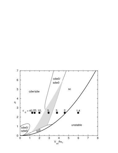
Figure 1: The phase diagram for the thinest zigzag carbon nanotubes in a parameter space given by the average bare interaction $V_{\rm av}/\hbar v_{F}$ and the ratio $\eta=v^{0}_{F}/v_{F}$ of the Fermi velocities. The sector of the diagram with the dominant superconducting fluctuations in the $j=1$ and $2$ ($j=0$) bands is marked by SC (SC0) and the portion with the dominant charge/spin density wave fluctuations in the $j=1$ and $2$ ($j=0$) bands is indicated by CDW/SDW (CDW0/SDW0). The gray area shows the metallic phase where all of the two-particle fluctuations are suppressed. The thick solid line points out the Bardeen-Wentzel instability. Large dots represent the averages for the bare interactions (2) with different $\epsilon_{d}$.

In Fig. 1 we present a phase diagram at zero temperature in the parameter space defined by the average bare interaction $V_{\rm av}$ (in units of $\hbar v_{F}$) and the ratio $\eta=v_{F}^{0}/v_{F}$. For large $\eta$ ($\gtrsim 6$) and small $V_{\rm av}/v_{F}$ the density wave fluctuations (DWFs) in the $j=1$ and $2$ bands appear to have the longest decaying length. For moderate $V_{\rm av}/\hbar v_{F}$, the DWFs dominate in the $j=0$ band and finally there is a wide part of the diagram where the SCFs develop in the $j=1$ and $2$ bands. This phase is terminated by the line where the BWI occurs. For moderate $\eta$, an additional phase appears where all kind of the two-particle fluctuations are suppressed (the gray area in Fig. 1). For small $\eta$ and $V_{\rm av}/\hbar v_{F}$, the DWFs evolve in the $j=0$ band and for larger $V_{\rm av}/\hbar v_{F}$, close to the BWI line, the SCFs are amplified in the $j=0$ band.

The SCFs with the longest decaying length develop in a band with a smaller renormalized velocity. In other bands, with a larger renormalized velocity, the SCFs are also amplified (with $\beta_{j}<2$). However, when the SCFs are enhanced, the DWFs are suppressed (with $\beta_{j}>2$) in all of the bands. Since $K_{0s}=K_{\nu}=1$, the exponents in the SSC and the TSC correlation functions are the same. This is also the case for the CDW/SDWz and the SDWs correlation functions. Further analysis, including the renormalization of the Luttinger liquid parameters due to backscattering processes, would resolve which particular correlation function has the longest decaying length.

We estimate the average value $V_{\rm av}$ of the bare interaction for the different dielectric constants $\epsilon_{d}$ of the zeolite host. We take the radius of the SWNT $a=2.1\AA$ and the radius of the 1-d cavity in the host $R=3.7\AA$ Qin00 ; Tang01 . The Fermi velocities are taken $v^{0}_{F}=6.9\cdot 10^{5}\;m/s$ and $v_{F}=2.8\cdot 10^{5}\;m/s$ Blase94 , which give the ration $\eta=2.46$. The dielectric constant for an isolated SWNT is $\epsilon_{1}=1.4$ Egger97 . The average potential decreases with increasing $\epsilon_{d}$ as is shown by dots going from the right to the left in Fig.1. For $\epsilon_{d}=\epsilon_{1}=1.4$, our estimation predicts that the metallic phase is unstable. For $\epsilon_{d}=2$ and $3$, the system is metallic and dominated by the SCFs. For $\epsilon_{d}=5$, we find that all two-particle fluctuations are suppressed. For $\epsilon_{d}=10,20$ and $40$, the DWFs appear to be dominant.

Dielectric properties of the host can change the physical properties of the SWNT. Creating and investigating electrical properties of the SWNTs in zeolites with different dielectric constants would be a direct verification of our theory. For the zeolite AlPO₄-5 with the dielectric constant $\epsilon_{d}\approx 2-4$, our theory predicts that the SCFs are amplified according to the experiment Tang01 . The dielectric constant of this zeolite after filling it in with the water is $\epsilon_{d}\approx 40$ zeolite . If one can still synthesis the SWNTs there, they should develop the DWFs.

In conclusion, fabricating the SWNTs inside the zeolite hosts with different dielectric constants would provide a rare opportunity to control the electron-electron interaction and to examine the different phases in such 1-d systems.

It is a pleasure to thank Prof. D. Vollhardt for discussion. Also information from Prof. P. Sheng on the experiment Tang01 are kindly acknowledged. This work was supported by the Alexander von Humboldt-Foundation.

References

- (1) S. Iijima, Nature 354, 56 (1991).
- (2) Physics Word, pp.29-53, Special issue - June (2000); and references therein.
- (3) R. Saito, G. Dresselhause, M.S. Dresselhause, Physical properties of carbon nanotubes (Imperial College Press, London 1998).
- (4) L-Ch. Qin et al., Nature 408, 50 (2000); N. Wang et al., ibid. 408, 51 (2000).
- (5) Z.K. Tang et al., Science 292, 2462 (2001).
- (6) R. Egger et al., Phys. Rev. Lett. 79, 5082 (1997); C.L. Kane et al., ibid. 79 5086 (1997); R. Egger et al., Eur. Phys. J. B3, 281 (1998); H. Yoshioka et al., Phys. Rev. Lett. 82, 374 (1999).
- (7) J. González, Phys. Rev. Lett. 88, 076403-1 (2002); cond-mat/ 0204171.
- (8) A. Sédéki et al., Phys. Rev. B 65, 140515-1 (2002).
- (9) M. Kociak et al., Phys. Rev. Lett. 86, 2416 (2001).
- (10) M. Quyang et al., Science 292, 702 (2001).
- (11) X. Blase et al., Phys. Rev. Lett. 72, 1878 (1994); O. Gülseren et al., Phys. Rev. B 65, 153405-1 (2002); K. Kanamitsu et al., J. Phys. Soc. of Japan 71, 483 (2002).
- (12) K. Byczuk et al., Phys. Rev. 60, 1507 (1999).
- (13) M.R.S. Tavares, et al., Phys. Rev. B 63, 045324-1 (2001).
- (14) Due to the time reversal symmetry the matrix elements . Additionally, in the limit the fast-oscillating terms can be neglected and the polarization functions . Also, because of the degeneracy between the bands, .
- (15) Formally, the potential should be slightly different from that given in the text because in deriving the effective Hamiltonian (3) one should terminate the renormalization of the interaction at some finite energy . However, the difference should be small and can be disregarded in the following.
- (16) F.D.M. Haldane, J. Phys. C 14, 2585 (1981); V.J. Emery et al., Phys. Rev. B 59, 15641 (1999).
- (17) The coefficients in the Bogoliubov transformation diagonalizing (6) are given by .
- (18) G. Wentzel, Phys. Rev. 83 168 (1951); J. Bardeen, Rev. Mod. Phys. 23, 261 (1951).
- (19) D. Loss et al., Phys. Rev. B 50, 12160 (1994); T. Martin et al., Int. J. Mod. Phys. B 9, 495 (1995).
- (20) M. Bockrath et al., Nature 397, 598 (1999); Z. Yao et al., ibid. 402, 273 (1999).
- (21) Explicitly, , , , and , where the upper (lower) sign corresponds to ().
- (22) Ch. Stenzel et al., J. of Microwave Power & Electromagnetic Energy 36, 155 (2001).