Dynamical properties of model communication networks

Abstract

We study the dynamical properties of a collection of models for communication processes, characterized by a single parameter $\xi$ representing the relation between information load of the nodes and its ability to deliver this information. The critical transition to congestion reported so far occurs only for $\xi=1$. This case is well analyzed for different network topologies. We focus of the properties of the order parameter, the susceptibility and the time correlations when approaching the critical point. For $\xi<1$ no transition to congestion is observed but it remains a cross-over from a low-density to a high-density state. For $\xi>1$ the transition to congestion is discontinuous and congestion nuclei arise.

I Introduction

The interaction between the elements of social, technological, biological, chemical and physical systems usually defines complex networks. The study of topological properties in such networks has recently generated a lot of interest among the scientific community watts98 ; barabasi99 ; amaral00 ; albert02 ; dorogovtsev?? . Part of this interest comes from the attempt to understand the behavior of technology based communication networks such as the Internet faloutsos99 , the World Wide Web albert99 ; huberman99 , e-mail networks ebel?? or phone call networks adamic01 . The study of communication processes is also of interest in other fields, notably in the design of organizations radner93 ; decanio98 . It is estimated that more than one-half of the U.S. work force is dedicated to information processing, rather than to make or sell things in the narrow sense radner93 .

Tools taken from statistical mechanics are used to understand not only the topological properties of these communication networks, but also their dynamical properties. Particularly interesting is the phenomenon of congestion. In has been observed, both in real networks jacobson88 and in model communication networks, ohira98 ; tretyakov98 ; arenas01 ; sole01 that the system only behaves efficiently when the amount of information handled is small enough. The network collapses above a certain threshold and some information is accumulated and remains undelivered over large time periods—or it is simply lost. This transition from a free to a congested regime is indeed a phase transition and could be related to the appearance of the $1/f$ noise observed in Internet flow data csabai94 ; takayasu96 .

Understanding congestion is also important from an engineering point of view. For instance, in October of 1986, during the first Internet collapse reported in the literature, the speed of the connection between the Lawrence Berkeley Laboratory and the UC at Berkeley—separated by 200 meters— dropped by a factor of 100 jacobson88 . Although the problem of congestion, and in particular its prevention and control jacobson88 , has been studied because of its implications in digital communications, a deep understanding of the physics of congestion for general communication processes and beyond particular protocols is still lacking.

A general collection of models that captures the essential features of communication processes has been recently proposed arenas01 . In these models, agents—nodes—are organized in a hierarchical network—a Cayley tree— and interchange information packets. Each agent has a certain capability that decreases as the number of packets to deliver increases. When the capability is inversely proportional to the number of accumulated packets, a continuous phase transition was found between the free and the congested phases. This transition was characterized by means of an order parameter.

The aim of this paper is to study the collection of models mentioned above, since only hierarchical lattices and a very particular congestion behavior—capability inversely proportional to the number of accumulated packets—were considered. An extension to consider the existence of cost to maintain communication channels has already been done guimera01 . First, the network model is extended beyond purely hierarchical Cayley trees. In particular, 1-dimensional and 2-dimensional lattices are considered. It should be noted that simple models such as Cayley trees and regular lattices can capture the main characteristics of the dynamics of information flow in complex networks. Hierarchical trees have been considered to model the TCP/IP protocol in the Internet csabai94 ; takayasu96 . On the other hand, computer based communication networks have been described by placing routers and servers in square lattices ohira98 ; sole01 .

Moreover it is shown that, independently of the topology, the collection of models can be split into three groups according to how the network collapses. In the first group, agents deliver more packets as they are more congested—although their capability, as defined in arenas01 , decreases—, and the network never collapses. In the second group, agents deliver always the same number of packets independently of their load—number of packets to deliver—; this behavior leads to a continuous phase transition as reported for hierarchical lattices in arenas01 . Finally, when agents deliver fewer packets as their loads increase, the transition to the congested phase is discontinuous and the network collapses in an inhomogeneous way giving rise to congestion nuclei. To characterize these behaviors, the order parameter defined in arenas01 is used, but also the power spectrum of the fluctuations and a susceptibility-like function. Most of the current effort is focused on the quantitative study of the continuous transition and the critical behavior associated to such a transition.

The paper is organized as follows. Section 2 presents the collection of models and describes some details concerning the extension beyond hierarchical lattices, including 1D and 2D lattices. In section 3, these models are studied numerically and analytically. The scaling of the critical point with the size of the system, the behavior of the order parameter, and the divergence of the characteristic time at the critical point are studied in detail. Finally, section 4 includes the discussion of the results and the conclusions.

II The model

The model considers three basic components: (i) the physical support for the communication process—agents and communication channels—, (ii) the discrete information packets that are interchanged, and (iii) the limited capability of the agents to handle such packets.

The communication network is mapped onto a graph where nodes mimic the communicating agents (for instance, employees in a company, routers and servers in a computer network, etc.) and the links between them represent communication lines. In particular, the three different topologies depicted in Fig. 1 are considered: 1D lattices of length $L$, 2D square lattices of side length $L$ and size $S=L^{2}$, and hierarchical Cayley trees with branching $z$ and a number of generations or levels $m$, hereafter denoted $(z,m)$.

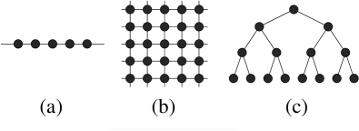
Figure 1: Network topologies studied. (a) 1D lattice with $L=5$; (b) 2D lattice with $L=5$ and $S=25$; and (c) $(2,3)$ Cayley tree with branching $z=2$ and $m=3$ levels or generations.

The dynamics of the model is as follows. At each time step $t$, an information packet is created at every node with probability $p$. Therefore $p$ is the control parameter: small values of $p$ correspond to low density of packets and high values of $p$ correspond to high density of packets. When a new packet is created, a destination node, different from the origin node, is chosen randomly in the network. Thus, during the following time steps $t+1,\,t+2,\ldots,\,t+T$, the packet travels toward its destination. Once the packet reaches the destination node, it is delivered and disappears from the network.

The time that a packet remains in the network is related not only to the distance between the source and the target nodes, but also to the amount of packets in its path. In particular, at each time step, all the packets move from their current position, $i$, to the next node in their path, $j$, with a probability $q_{ij}$. This probability $q_{ij}$ is called the quality of the channel between $i$ and $j$, and was defined in arenas01 as

$$q_{ij}=\sqrt{k_{i}k_{j}}\,,$$ (1)

where $k_{i}$ represents the capability of agent $i$ at each time step. The quality of a channel is, thus, the geometric average of the capabilities of the two nodes involved, so that when one of the agents has capability 0, the channel is disabled. High qualities ($q_{ij}\approx 1$) imply that packets move easily while low qualities ($q_{ij}\approx 0$) imply that it takes a long time for a packet to jump from one node to the next. The general equation proposed for $k_{i}$ is:

$$k_{i}=f(n_{i})$$ (2)

where $n_{i}$ is the total number of packets currently at node $i$. The function $f(n)$ determines how the capability evolves when the number of packets at a given node changes,

$$f(n)=\left\{\begin{array}[]{lcl}1&\quad\mbox{for}&n=0\\ n^{-\xi}&\quad\mbox{for}&n=1,2,3,\ldots\end{array}\right.$$ (3)

with $\xi\geq 0$. Equation (3) defines a complete collection of models with agents that behave differently depending on the exponent $\xi$.

The average number of packets delivered during one time step by a node $i$ to another node $j$ is proportional to $n_{i}/(n_{i}^{\xi/2}n_{j}^{\xi/2})$. Assuming that $n_{i}\propto n_{j}$ the former expression reads $n_{i}^{1-\xi}$. The proportionality is exact both in the hierarchical lattice and in large enough 1D and 2D lattices, where adjacent nodes are statistically equivalent.

Therefore, for $\xi<1$ the number of delivered packets increases with the number of accumulated packets. For $\xi>1$ the number of delivered packets decreases as the number of accumulated packets increases. Finally, for the particular case $\xi=1$, the number of delivered packets is independent of the number of accumulated packets. Note that this particular case is consistent with simple models of queues ohira98 .

The last point that needs to be explained to completely define the current model is the routing algorithm or, in other words, the set of rules that the nodes follow to select where to send a certain packet. In all the topologies considered (1D, 2D and Cayley) the packets follow paths of minimum length from their origin to their destination—open boundary conditions are set in both 1D and 2D networks. In 1D lattices and Cayley trees it is trivial to follow a minimum path because there is only one minimum path between two arbitrary nodes. In 2D lattices, however, there are many minimum paths. If a node can choose between two neighbors when sending a given packet, and both neighbors belong to a minimum path between the origin and the destination of the packet, one of them is chosen randomly with equal probability. This algorithm is indeed the simplest one and the interpretation of the results is clearer than for more complex routing algorithms. However, congested nodes will still have lower probability of receiving packets because of the definition of the quality of a channel. Therefore packets will avoid those nodes to some extent, as would happen in more sophisticated routing algorithms.

III Results

For certain parameters of the model (in particular $\xi=1$ arenas01 ) and for similar models of traffic ohira98 , a transition from a free regime, where all the packets reach their destination, to a congested, regime where some packets are accumulated in the network, has been found. This transition is properly described by means of the following order parameter $\eta(p)$ introduced previously arenas01 :

$$\eta(p)=\lim_{t\rightarrow\infty}\frac{1}{pS}\frac{\left\langle\Delta N\right\rangle}{\Delta t}$$ (4)

In this equation $\Delta N=N(t+\Delta t)-N(t)$ and $\langle\ldots\rangle$ indicates average over time windows of width $\Delta t$. These averages can be over one or many realizations, yielding the same result. Essentially, the order parameter represents the ratio between undelivered and generated packets calculated at long enough times such that $\Delta N\propto\Delta t$. Thus, $\eta$ is only a function of the probability of packet generation per node and time step, $p$.

The power spectrum $S(f)$ of the total number of packets in the network $N(t)=\sum_{i}n_{i}$ is also used here to further understand the phase transition. By means of the power spectrum the behavior of the time correlations of the system can be studied.

Let us study separately the critical case $\xi=1$ and the non critical cases $\xi<1$ and $\xi>1$.

III.1 The critical case $\xi=1$

A continuous transition between the free regime and the congested regime occurs in hierarchical networks for $\xi=1$, as reported in arenas01 . For small values of $p$, all the packets reach their destination and the total number of packets $N(t)$ fluctuates around a finite value. In this case the order parameter is $\eta=0$. However, as $p$ increases, a critical point $p_{c}$ is reached, where the fluctuations in $N(t)$ become very large and the characteristic time of the system diverges (critical slowing down). Beyond this point, some packets remain undelivered and $\langle N(t)\rangle$ grows linearly with $t$. The same qualitative behavior is observed here for 1D and 2D lattices, although there are quantitative differences.

From an engineering point of view it is interesting to study first the behavior of $p_{c}$ as the number of nodes in the network $S$ changes, because it will provide valuable information about the scalability of the network. Note that $N_{c}=p_{c}S$ is the maximum number of packets that the network can handle per time step and, thus, it is a measure of the capacity of the network.

For the hierarchical Cayley tree, a mean field calculation of $p_{c}$ was obtained in arenas01 :

$$p_{c}^{CT}=\frac{\sqrt{z}}{\frac{z(z^{m-1}-1)^{2}}{z^{m}-1}+1}\approx\frac{z^{3/2}}{(z-1)}\frac{1}{S}\mbox{ ,}$$ (5)

where the approximation holds for $z^{m-1}\gg 1$.

It is also possible to derive a mean field expression of $p_{c}$ for the 1D lattice. Since the most congested node is, from symmetry arguments, the central one—the node at $\ell=L/2$—, the network will collapse when the amount of packets received by this central node is higher than the maximum number of packets that it is able to deliver. Since in a large enough network it is safe to assume that the central node will be congested similarly to its neighbors, $n_{\ell-1}=n_{\ell}=n_{\ell+1}$, the maximum number of delivered packets should be 1. On the other hand, the number of packets arriving to the central node at each time step is the number of packets that are generated at each time step at the left half of the network and have their destination at the right half and conversely, this is $pL/2$. Then the critical condition is given by

$$1=\frac{p_{c}^{1D}L}{2}\Rightarrow p_{c}^{1D}=\frac{2}{L}.$$ (6)

These mean field expressions (5) and (6) can be compared with simulations. Nevertheless, the fluctuations of $N(t)$ become very large near $p_{c}$ and it is difficult to calculate the value of the order parameter. Instead, a susceptibility-like function $\chi(p)$ can be defined by analogy with equilibrium thermal critical phenomena, and used to estimate more accurately the value of the critical probability of packet generation, $p_{c}$. The susceptibility $\chi$ is related to the fluctuations of the order parameter by

$$\chi(p)=\lim_{T\rightarrow\infty}T\sigma_{\eta}(T)$$ (7)

where $T$ is the width of a time window, and $\sigma_{\eta}(T)$ is the standard deviation of the order parameter estimated from the analysis of many different time windows of width $T$. Thus a calculation implies a long realization of $N(t)$, its division into windows of width $T$, calculation of the average value of the order parameter in each window and finally the determination of the standard deviation of these values. The susceptibility shows (Fig. 2) a singularity at $p_{c}$ as $T$ grows, as expected.

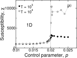
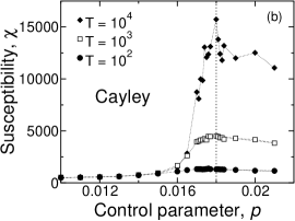
Figure 2: Susceptibility for (a) a 1D lattice with $L=100$ and (b) a (5,4) Cayley tree, for different time windows $T$. The vertical dotted line corresponds to the mean field calculation of the critical point (equations (6) and (5) respectively.)

Fig. 3 shows that there is good agreement between expressions (5) and (6) and the values of $p_{c}$ obtained numerically by means of susceptibility measures for different network sizes.

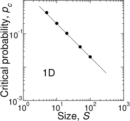
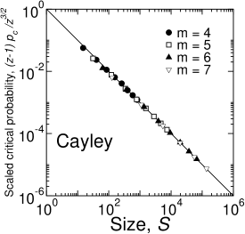
Figure 3: Comparison between analytical (lines) and numerical (symbols) values of $p_{c}$ obtained for the (a) 1D and (b) the Cayley trees. The error bars of the numerical points are smaller than the size of the symbols.

For the 2D lattice it is more difficult to obtain even a mean field expression for $p_{c}$. However, since for 1D lattices and Cayley trees the scaling relation $p_{c}\propto S^{-1}$ holds—where $S$ is the size of the network—, one may expect the same behavior for the 2D lattice. Using the susceptibility to numerically determine $p_{c}$ from simulations, one finds that this turns out to be incorrect. Although it is difficult to obtain a precise value of the exponent, Fig 4 shows that it is close to 0.6 instead of 1.0:

$$p_{c}^{2D}\propto S^{-0.6}.$$ (8)

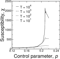
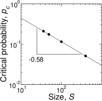
Figure 4: (a) Susceptibility for a 2D $6\times 6$ lattice. (b) Scaling of the critical probability of packet generation as a function of the size of the system for 2D square lattices.

This result suggests that the existence of multiple paths to get from the origin to the destination has important consequences, not only in shifting the value of $p_{c}$, but actually changing its critical scaling behavior.

The behavior of the order parameter is studied next. It is possible to derive an analytical expression for the simplest 1D case where there are only two nodes that exchange packets. Since from symmetry considerations $n_{1}=n_{2}$, the average number of packets eliminated in one time step is $2$, while the number of generated packets is $2p$. Thus $p_{c}=1$ and with the present formulation of the model it is not possible to reach the super-critical congested regime. However, $p$ can be extended to be the average number of generated packets per node at each step (instead of a probability) and in this case it can actually be as large as needed. As a result, the order parameter for the super-critical phase is $\eta=(p-1)/p$. As observed in Fig. 5, the general form

$$\eta(p/p_{c})=\frac{p/p_{c}-1}{p/p_{c}}$$ (9)

fits very accurately the behavior of the order parameter not only for this simple 1D lattice with $L=2$ or the Cayley tree arenas01 , but also for any 1D lattice. Two-dimensional lattices again deviate from this behavior, although the deviation is small.

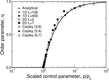
Figure 5: Behavior of the order parameter in the case $\xi=1$. The solid line corresponds to the analytical calculation for two nodes exchanging information packets. Symbols correspond to simulations performed in 1D, 2D and Cayley lattices.

In particular, near $p_{c}$, equation (9) implies

$$\eta(p)\propto(p-p_{c})$$ (10)

and thus the critical exponent for the order parameter is equal to 1 at least for the 1D lattice and the Cayley tree.

The analysis of the power spectrum shows that in the sub-critical regime, i.e. in the free phase, the spectrum is well fitted by a Lorentzian characterized by a frequency, $f_{c}$, corresponding to exponentially decaying correlations with a characteristic time $\tau$, as depicted in Fig. 6. As $p$ approaches $p_{c}$, it is observed that $f_{c}\rightarrow 0$ and the power spectrum becomes $1/f^{2}$ for the whole range of frequencies. Alternatively the characteristic time diverges as $\tau\rightarrow\infty$ (critical slowing down). This qualitative behavior is common to all the topologies of the underlying network, as shown in Fig. 6.

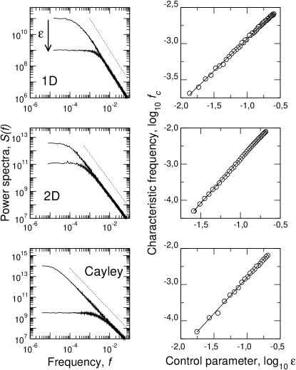
Figure 6: Left: Log-Log plot of the power spectrum of $N(t)$ for different topologies and different values of the control parameter $\epsilon=(p_{c}-p)/p_{c}$ for the 1D case ($L=100$), 2D case ($L=6$), and Cayley $(7,5)$. Power spectra have been obtained averaging over 100 realizations of $N(t)$. Dotted lines represent a power law with exponent -2. Right: Characteristic frequency as a function of the control parameter $\epsilon$ for the different topologies. As observed, the characteristic frequency tends to 0 as $p\rightarrow p_{c}$ following a power law. The straight lines correspond to fittings of equation (11).

It is interesting to study how the characteristic frequency drops to 0 for each network topology. Near the critical point, one expects the scaling behavior

$$f_{c}\propto(p_{c}-p)^{\gamma}.$$ (11)

The value of the critical exponent $\gamma$ can be estimated by fitting Eq. (11) to values of $f_{c}(p)$ close enough to the critical point, as shown in Fig. 6. Note that we fit $p_{c}$ and $\gamma$ simultaneously. This procedure yields very accurate values of $p_{c}$ but the values of $\gamma$ are subject to large errors. Fig. 6 yields $\gamma\approx 0.9$ for a 1D network with $L=100$, $\gamma\approx 2.5$ for a 2D network with $L=7$, and $\gamma\approx 2$ for a (7,5) Cayley tree.

The determination of $\gamma$ is interesting not only from an academic point of view, but also from an engineering perspective. Indeed, this exponent is related to divergences of other relevant quantities near the critical point. Any characteristic time $\tau$—the average time to deliver a packet, for instance—will diverge as

$$\tau\propto(p_{c}-p)^{-\gamma}$$ (12)

and similarly the total number of packets

$$N\propto(p_{c}-p)^{-\gamma}$$ (13)

since

$$\frac{N}{\tau}=pS$$ (14)

from Little’s law allen90 . This law states that, in steady state, the number of delivered packets and the number of generated packets are equal.

The estimation of $\gamma$ is particularly interesting in electronic communication protocols. Indeed, Eq. (12) is used to determine the waiting time before a packet is considered lost in the network and therefore sent again jacobson88 . In practice, the exponent $\gamma=1$ predicted by classical queue theory allen90 is assumed, while our current results suggest that more complex settings can lead to exponents even larger than 2.

III.2 Non critical cases $\xi<1$ and $\xi>1$

We have shown that the number of packets delivered by node $i$ is $n_{i}^{1-\xi}$ and thus, when $\xi<1$, it increases with the number of packets that this node accumulates. It is difficult to imagine a real scenario with this characteristic. However, this case has been included to understand the critical behavior when $\xi=1$, i.e., to show the relationship between criticality and the amount of packets that can be delivered when load increases. As a consequence of the increase of the deliver capability with the load, the transition to collapse will never occur because, at some point in time, the number of accumulated packets will be large enough and the number of delivered and created packets will balance each other. Thus, the order parameter will be zero for any value of the control parameter $p$, and the correlations will decay exponentially. As shown in Fig. 7, the characteristic frequency tends asymptotically to $f_{c}^{*}$ as $p$ increases. This asymptotic value depends on the size of the system.

For a 1D lattice with a high density of packets ($p\rightarrow 1$), the number of packets that are delivered by a node is $n_{i}^{1-\xi}$ while the number of packets that are being delivered to this node is proportional to $L$ (for instance, for the central node, this number is simply $pL/2$). Therefore, $n_{i}\propto L^{1/(1-\xi)}$. The total number of packets is $N=\sum_{i}n_{i}\sim L^{1+1/(1-\xi)}$ and according to Little’s Law

$$f_{c}^{*}\propto\frac{pL}{N}\propto L^{\frac{-1}{1-\xi}}$$ (15)

On the other hand, for $p\rightarrow 0$ the scaling of the characteristic frequency is given by

$$f_{c}^{0}\propto L^{-1}$$ (16)

since the packets success to jump from one node to the next at each time step, and therefore the characteristic time is directly the average path length between nodes.

Therefore, although there is no phase transition in this case $\xi<1$, there is a cross-over from a low density behavior to a high density behavior, as shown in Fig. 7. This crossover is also observed in 2D lattices and Cayley trees.

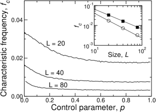
Figure 7: Characteristic frequency $f_{c}$ as a function of the probability of packet generation $p$, for $\xi=0.2$ and different sizes of a 1D lattice. As observed, $f_{c}$ never becomes 0 as happens in the critical $\xi=1$ case. Inset: Characteristic frequency at $p\rightarrow 0$, $f_{c}^{0}$ (squares), and characteristic frequency at large $p$, $f_{c}^{*}$ (circles). The lines represent the fittings provided by equation (16) $f_{c}^{0}\propto L^{-1}$, and equation (15) $f_{c}^{*}\propto L^{-1/(1-\xi)}$, respectively.

The phase transition observed for $\xi=1$ is recovered when $\xi>1$. Above a certain threshold, some packets are accumulated in the network and the order parameter differs from 0. However, the number of packets delivered by a node $i$ in this case $\xi>1$ decreases with the number of packets accumulated at that node. Therefore, when some packets are accumulated, $n_{i}$ grows and finally no packets are delivered at all. Thus suddenly above the transition, which is discontinuous, the order parameter becomes 1.

The change in the order of the phase transition affects the spreading of the collapse over the network. In the critical case $\xi=1$, the collapse starts at the most central node and then spreads from this point to the rest of the network. In this case $\xi>1$, the reinforcement effect—the fact that the more collapsed a node is, the more collapsed will get in the future—leads to the formation of many congestion nuclei generated by fluctuations, that spread over the whole network. Figure 8 illustrates the formation of these congestion nuclei for 2D lattices with $\xi=5$ and $p=0.001$, and $\xi=2$ and $p=0.01$

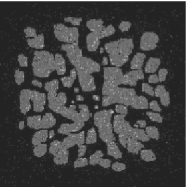
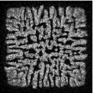
Figure 8: Congestion nuclei formation for large 2D lattices of $L=200$, in the non critical case $\xi>1$. Dark regions represent regions with small congestion levels while bright regions correspond to highly congested regions. Left: $\xi=5$ and $p=0.001$. Right: $\xi=2$ and $p=0.01$.

IV Discussion and conclusions

A collection of models recently proposed for hierarchical networks arenas01 has been examined in detail for several network topologies including 1D and 2D lattices, to characterize the phase transition to collapse. New congestion scenarios have been analyzed.

First, it has been shown that the congestion behavior is governed by the ability of agents to deliver information packets when their load increases. When agents deliver packets at a constant ratio independently of their load—number of packets to deliver—, a continuous transition as the one reported in arenas01 for Cayley trees is also observed for 1D and 2D lattices, the order parameter being the fraction of accumulated packets. When the number of delivered packets increases with the load, no phase transition is observed. Conversely, when the number of delivered packets decreases with the load, the order parameter jumps from zero to one and the transition becomes discontinuous. These different behaviors are tuned by a single parameter $\xi$, which is the exponent that determines how the capability of nodes evolves with the number of accumulated packets. When $\xi<1$ there is no transition to the congested regime, for $\xi=1$ the transition is continuous and for $\xi>1$ the transition is discontinuous. Note that the continuous transition (reported in arenas01 and in some models of queues tretyakov98 ; sole01 ) is only a particular case between a no-congestion behavior and a discontinuous transition behavior. Thus, the critical behavior is intimately related to the independence between load and deliver capability of nodes.

These different behaviors have been analyzed separately. The critical case $\xi=1$ presents the most interesting behavior. To properly understand the physics of the collapse process it is necessary to know how the system approaches the critical point. The order parameter becomes useless in this region due to the emergence of large fluctuations, and then we have defined a susceptibility-like function that is related, by analogy to equilibrium critical phenomena, to fluctuations of the order parameter. This quantity shows a peak at the critical point and allows to study the dependence on the size and topology of the system. For 1D lattices and Cayley trees, it has been shown (by means of simulation and also with mean field calculations) that $p_{c}$ scales as the inverse of the size of the system, $p_{c}\propto S^{-1}$. However, for 2D lattices a different scaling $p_{c}\propto S^{-0.6}$ is obtained. It is suggested that the existence of multiple paths from the origin to the destination of the packets is the responsible for this change in the scaling behavior. On the other hand, the study of the power spectrum of the number of the packets in the network as a function of time has provided valuable information about the variation of temporal correlations in the system. In particular, below $p_{c}$ correlations decay exponentially, with a characteristic time $\tau$ that diverges at $p_{c}$. The exponent of this divergence is significantly larger than what is expected from queue theory. This can be relevant to accurately forecast the temporal behavior in complex communication settings.

For $\xi<1$, no phase transition is observed. Instead, a cross-over from a low-density to a high-density regime occurs. In the low density regime, the characteristic frequency is determined by the average distance between nodes, while in the high density regime the characteristic frequency is determined by the capability of agents to deliver information packets. In 1D lattices, the cross-over changes the scaling from $f_{c}\propto L^{-1}$ at low densities to $f_{c}\propto L^{-1/(1-\xi)}$ at high densities.

Finally, when $\xi>1$ the transition to the congested regime is discontinuous, since the number of delivered packets decreases with the load and for long times no packets are delivered at all. Thus the order parameter jumps from 0 to 1. Moreover, due to the reinforcement effect—the fact that the more collapsed a node is, the more collapsed it will get in the future—leads to the formation of many congestion nuclei generated by fluctuations, that spread over the whole network. The existence and distribution of such congestion nuclei can also be of interest from an engineering point of view.

- (1) D. Watts and S. Strogatz, Nature 393, 440 (1998).
- (2) A.-L. Barabasi and R. Albert, Science 286, 509 (1999).
- (3) L. A. N. Amaral, A. Scala, M. Barthelemy, and H. E. Stanley, Proc. Nat. Acad. Sci. 97, 11149 (2000).
- (4) R. Albert and A.-L. Barabasi, Reviews of Modern Physics 74, 47 (2002).
- (5) S. Dorogovtsev and J. F. F. Mendes, Preprint cond-mat/0106144 (2001).
- (6) M. Faloutsos, P. Faloutsos, and C. Faloutsos, Comp. Comm. Rev. 29, 251 (1999).
- (7) R. Albert, H. Jeong, and A.-L. Barabasi, Nature 401, 130 (1999).
- (8) B. Huberman and L. Adamic, Nature 401, 131 (1999).
- (9) H. Ebel, L.-I. Mielsch, and S. Bornholdt, Preprint cond-mat/0201476 (2002).
- (10) L. A. Adamic, R. M. Lukose, A. R. Puniyani, and B. A. Huberman, Physical Review E 64, 046135 (2001).
- (11) R. Radner, Econometrica 61, 1109 (1993).
- (12) S. DeCanio and W. Watkins, Journal of Economic Behavior and Organization 36, 275 (1998).
- (13) V. Jacobson, in Proceedings of SIGCOMM ’88 (ACM, Standford, CA, 1988).
- (14) T. Ohira and R. Sawatari, Physical Review E 58, 193 (1998).
- (15) A. Tretyakov, H. Takayasu, and M. Takayasu, Physica A 253, 315 (1998).
- (16) A. Arenas, A. Diaz-Guilera, and R. Guimera, Physical Review Letters 86, 3196 (2001).
- (17) R. Sole and S. Valverde, Physica A 289, 595 (2001).
- (18) I. Csabai, Journal of Physics A: Mathematical and General 27, L417 (1994).
- (19) M. Takayasu, H. Takayasu, and T. Sato, Physica A 233, 824 (1996).
- (20) R. Guimera, A. Arenas, and A. Diaz-Guilera, Physica A 299, 247 (2001).
- (21) O. Allen, Probability, statistics and queueing theory with computer science application, 2nd ed. (Academic Press, New York, 1990).