Finite Size Scaling analysis of the avalanches in the 3d Gaussian Random Field Ising Model with metastable dynamics

Abstract

A numerical study is presented of the 3d Gaussian Random Field Ising Model at $T=0$ driven by an external field. Standard synchronous relaxation dynamics is employed to obtain the magnetization versus field hysteresis loops. The focus is on the analysis of the number and size distribution of the magnetization avalanches. They are classified as being non-spanning, 1d-spanning, 2d-spanning or 3d-spanning depending on whether or not they span the whole lattice in the different space directions. Moreover, finite-size scaling analysis enables identification of two different types of non-spanning avalanches (critical and non-critical) and two different types of 3d-spanning avalanches (critical and subcritical), whose numbers increase with L as a power-law with different exponents. We conclude by giving a scenario for avalanche behaviour in the thermodynamic limit.

I Introduction

Systems with first-order phase transitions exhibit a discontinuous change of their properties when driven through the transition point. Sometimes, due to the existence of energy barriers larger than thermal fluctuations, such systems evolve following a path of metastable states and exhibit hysteresis. Metastable phenomena develop more often in the case of systems at low temperature and with quenched disorder. In many cases the first-order phase transition occurs, instead of at a certain transition point, in a broad range of the driving parameter and the discontinuity is split into a sequence of jumps or avalanches between metastable states. Moreover, under certain conditions such avalanches do not show any characteristic spatial or time scale: the distribution of their size and duration becomes a power-law. This framework, which has sometimes been called fluctuationless first-order phase transitions Vives and Planes (1994); Carrillo et al. (1998), is one of the basic mechanisms responsible for power-laws in nature D.Sornette (2000). Experimental examples have been found in a broad set of physical systems: magnetic transitions P.J.Cote and L.V.Meisel (1991), adsorption M.P.Lilly et al. (1993), superconductivity W.Wu and P.W.Adams (1995), martensitic transformations Vives et al. (1994), etc.

A paradigmatic model for such fluctuationless first-order phase transitions in disordered system is the Gaussian Random Field Ising Model (GRFIM) at $T=0$ driven by an external field $H$. The amount of quenched disorder is controlled by the standard deviation $\sigma$ of the Gaussian distribution of independent random fields acting on each spin. Metastable evolution is obtained with appropriate local relaxation dynamics which assumes a separation of time scales between the driving field rate $dH/dt$ and the avalanche duration. The response of the system to the driving field can be followed by measuring the total magnetization $m(H)$. The response exhibits the above-mentioned metastable phenomena: hysteresis and avalanches.

Since the model was introduced some years ago Sethna et al. (1993); Dahmen and J.P.Sethna (1993), different studies (numerical and analytical) have been carried out in order to characterize the hysteresis loops $m(H)$ and the magnetization avalanches Perković et al. (1995); Dahmen and J.P.Sethna (1996); Tadić (1996); Perković et al. (1999); Kuntz et al. (1999); J.H.Carpenter and K.A.Dahmen (2002). Two of the most well-studied properties are the number of avalanches $N(\sigma)$ and the distribution $D(s;\sigma)$ of avalanche sizes $s$ along half a hysteresis loop. For large amounts of disorder ($\sigma>\sigma_{c}$) the loops look smooth and continuous. They consist of a sequence of a large number of tiny avalanches whose size distribution $D(s;\sigma>\sigma_{c})$ decays exponentially with $s$. On the other hand, for small amounts of disorder ($\sigma<\sigma_{c}$), besides a certain number of small avalanches, one or several large avalanches produce a discontinuity $\Delta m$ in the hysteresis loop. For an intermediate critical value $\sigma_{c}$ the distribution $D(s,\sigma_{c})$ of avalanche sizes $s$ can be approximated by a power-law: $D(s;\sigma_{c})\sim s^{-\tau}$.

Many of the properties of the GRFIM have been understood by assuming the existence of a $T=0$ critical point $(\sigma_{c},H_{c})$ on the metastable phase diagram. The more recent estimation Perković et al. (1999) renders: $\sigma_{c}=2.16\pm 0.03$ and $H_{c}=1.435\pm 0.004$. Although partial agreement on the values of the critical exponents has been reached, other features are still controversial.

One of the fundamental problems is the definition of the order parameter. From a thermodynamic point of view the discontinuity of the hysteresis loop $\Delta m$ seems to be an appropriate order parameter if $\Delta m>0$ for $\sigma<\sigma_{c}$ and $\Delta m=0$ for $\sigma>\sigma_{c}$. Nevertheless, in the $T=0$ numerical simulations, due to the finite size of the system and for a given realization of disorder, all the magnetization changes are discontinuous. Note that this does not occur for standard thermal numerical simulations in which, due to thermal averaging, magnetization is continuous for finite systems. Only finite-size scaling analysis will reveal which are the “large avalanches” and whether or not avalanches become vanishingly small in the thermodynamic limit. It is thus very important to study the properties of the “spanning” avalanches. These are avalanches that, for a finite system with periodic boundary conditions, cross the system from one side to another. In particular it would be interesting to measure the number $N_{s}(\sigma)$ of spanning avalanches and their size distribution $D_{s}(s;\sigma)$.

A second unsolved question, related to the previous one, is the spatial structure of the avalanches. It has been suggested that they are not compact Perković et al. (1995); O.Perković et al. (1996). A fractal dimension ($d_{f}=1/0.34<3$) has been estimated from the avalanche size distribution Dahmen and J.P.Sethna (1996). It would be interesting to understand how such a fractal behaviour may, in the thermodynamic limit, represent a magnetization discontinuity.

A third problem is the definition of the scaling variables in order to characterize the critical properties close to the critical point $(\sigma_{c},H_{c})$. When focusing on the study of avalanche properties, it should be pointed out that the scaling analysis is performed by using quantities ($N(\sigma)$ and $D(s,\sigma)$) measured recording all the avalanches along half a hysteresis loop. The measurement of non-integrated distributions, i.e. around a certain value of $H$, will require large amounts computing effort in order to reach good statistics for large enough systems. Therefore, the dependence on the field $H$ is integrated out and the distance to the critical point $\sigma_{c}$ is measured by a single scaling variable $u(\sigma)$. Although in pioneering papers Sethna et al. (1993); Dahmen and J.P.Sethna (1993) the most usual scaling variable $u_{1}=\left(\sigma-\sigma_{c}\right)/\sigma_{c}$ was used in order to scale the avalanche size distribution, forthcoming studies Perković et al. (1995); Dahmen and J.P.Sethna (1996); Perković et al. (1999) changed the definition to $u_{3}=\left(\sigma-\sigma_{c}\right)/\sigma$. Apparently both definitions are equivalently close to the critical point, but it can be checked that the “phenomenological” scaling of the distributions $D(s;\sigma)$ using $u_{3}$ (with $u_{3}>0.04$) as suggested in the inset of Fig. 1 in Ref. Perković et al., 1995, is not possible when using $u_{1}$.

Finite-size scaling analysis has been carried out O.Perković et al. (1996); Perković et al. (1999) for the number of spanning avalanches $N_{s}(\sigma;L)$. Nevertheless, such finite-size scaling has not been presented either for the avalanche size distributions $D(s;\sigma,L)$ or for the number of non-spanning avalanches $N_{ns}(\sigma;L)$. Most of the studies Perković et al. (1995, 1999) have proposed collapses by neglecting the fact that simulated systems are finite. There is an exception Tadić (1996); B.Tadić and U.Nowak (2000) for which the scaling of the avalanche distributions with $L$ has been studied. In this case, nevertheless, the dependence on the distance to the critical point has been neglected and, consequently, parameter-dependent exponents have been obtained. In our opinion, scaling of the avalanche distribution must be studied on a two dimensional plane, including a scaling variable which accounts for the finite-size $L$ and another which accounts for the distance to the critical point.

Previous studies have provided simulations of very large system sizes (up to $L=1000$) Kuntz et al. (1999). This has been advantageous for the study of self-averaging quantities. Nevertheless, the properties of the spanning avalanches are non-self averaging. This is because, as will be shown, the number of spanning avalanches per loop does not grow as $L^{3}$. This means that, in order to obtain better accuracy, it is more important to perform averages over different disorder configurations (which will be indicated by $\langle\cdot\rangle$ ) than to simulate very large system sizes.

In this paper we present intensive numerical studies of the metastable 3d-GRFIM and focus on analysis of the spanning avalanches. In section II the model, the definition of a spanning avalanche and the details of the numerical simulations are presented. In section III raw numerical results are given. In section IV some of the Renormalization Group (RG) ideas will be reviewed, which will be taken into account for the analysis of the critical point. A finite-size scaling analysis of the avalanche numbers is presented in section V. The same analysis for size distributions and their $k$-moments are presented in sections VI and VII respectively. Section VIII presents a discussion on the behaviour of magnetization. The discussion of the results in relation with previous works is presented in section IX. Finally in section X a full summary and conclusions is given.

II Model

The 3d-GRFIM is defined on a cubic lattice of size $L\times L\times L$. On each lattice site ($i=1,\dots,L^{3}$) there is a spin variable $S_{i}$ taking values $\pm 1$. The Hamiltonian is:

$${\cal H}=-\sum_{i,j}^{n.n.}S_{i}S_{j}-\sum_{i=1}^{L^{3}}h_{i}S_{i}-H\sum_{i=1}^{L^{3}}S_{i}\;\;,$$ (1)

where the first sum extends over all nearest-neighbour (n.n) pairs, $H$ is the external applied field and $h_{i}$ are quenched random fields, which are independent and are distributed according to a Gaussian probability density

$$dP(h_{i})=\frac{1}{\sqrt{2\pi}\sigma}e^{-\frac{h_{i}^{2}}{2\sigma^{2}}}dh_{i}\;\;,$$ (2)

where the standard deviation $\sigma$, is the parameter that controls the amount of disorder in the system. Note that $\langle h_{i}\rangle=0$ and $\langle h_{i}^{2}\rangle=\sigma^{2}$.

The system is driven at $T=0$ by the external field $H$. For $H=+\infty$ the state of the system which minimizes $\cal H$ is the state with maximum magnetization $m=\sum_{i=1}^{L^{3}}S_{i}/L^{3}=1$. When the external field $H$ is decreased, the system evolves following local relaxation dynamics. The spins flip according to the sign of the local field:

$$h_{i}+H+\sum_{j=1}^{6}S_{j}\;\;,$$ (3)

where the sum extends over the 6 nearest-neighbouring spins of $s_{i}$. Avalanches occur when a spin flip changes the sign of the local field of some of the neighbours. This may start a sequence of spin flips which occur at a fixed value of the external field $H$, until a new stable situation is reached. $H$ is then decreased again. This “adiabatic” evolution corresponds to the limit for which avalanches are much faster than the decreasing field rate. Note that, once the local random fields are fixed, the metastable evolution is completely deterministic, no inverse avalanches may occur and the hysteresis loops exhibit the return point memory property Sethna et al. (1993).

The size of the avalanche $s$ corresponds to the number of spins flipped until a new stable situation is reached. Note that the corresponding magnetization change is $\Delta m=2s/L^{3}$.

For a certain realization of the random fields, corresponding to a given value of $\sigma$, we have recorded the sequence of avalanche sizes during half a hysteresis loop, i.e. decreasing $H$ from $+\infty$ to $-\infty$. The two main quantities (see Table 1) that are measured after averaging over different realizations of disorder, are the total number of avalanches per loop $N(\sigma,L)$ and the distribution of avalanche sizes $D(s;\sigma,L)$, normalized so that:

$$\sum_{s=1}^{L^{3}}D(s;\sigma,L)=1\;\;.$$ (4)

Note that given this normalization condition and the fact that $s$ is a natural number, then $D(s;\sigma,L)\leq 1$.

averaged number	notation
avalanches	$N(\sigma,L)$
spanning avalanches	$N_{s}(\sigma,L)$
non-spanning avalanches	$N_{ns}(\sigma,L)$
critical non-spanning avalanches	$N_{nsc}(\sigma,L)$
non-critical non-spanning avalanches	$N_{ns0}(\sigma,L)$
1d-spanning avalanches	$N_{1}(\sigma,L)$
2d-spanning avalanches	$N_{2}(\sigma,L)$
3d-spanning avalanches	$N_{3}(\sigma,L)$
critical 3d-spanning avalanches	$N_{3c}(\sigma,L)$
subcritical 3d-spanning avalanches	$N_{3-}(\sigma,L)$
normalized size distribution	notation
avalanches	$D(s;\sigma,L)$
spanning avalanches	$D_{s}(s;\sigma,L)$
non-spanning avalanches	$D_{ns}(s;\sigma,L)$
critical non-spanning avalanches	$D_{nsc}(s;\sigma,L)$
non-critical non-spanning avalanches	$D_{ns0}(s;\sigma,L)$
1d-spanning avalanches	$D_{1}(s;\sigma,L)$
2d-spanning avalanches	$D_{2}(s;\sigma,L)$
3d-spanning avalanches	$D_{3}(s;\sigma,L)$
critical 3d-spanning avalanches	$D_{3c}(s;\sigma,L)$
subcritical 3d-spanning avalanches	$D_{3-}(s;\sigma,L)$

Table 1: Notation of the studied quantities in this work. All the quantities refer to the analysis of half a hysteresis loop and are obtained after averaging over many different realizations of disorder.

The numerical algorithm we have used is the so-called brute force algorithm propagating one avalanche at a time Kuntz et al. (1999). We have studied system sizes ranging from $L=5(L^{3}=125)$ to $L=48(L^{3}=110592)$. The measured properties are always averaged over a large number of realizations of the random field configuration for each value of $\sigma$. Typical averages are performed over a number of configurations that ranges between $10^{5}$ for $L\leq 16$ to $2000$ for $L=48$.

We have used periodic boundary conditions: the numerical simulations correspond, in fact, to a periodic infinite system. Therefore, strictly speaking, all avalanches are infinite. Nevertheless, we need to identify which avalanches will become important in the thermodynamic limit. The definition that best matches this idea is the concept of spanning avalanches: those avalanches that, at least in one of the $x$, $y$ or $z$ directions, extend over the length $L$. This definition is very easy to implement numerically in the brute force algorithm. Spanning avalanches are detected by using three ($x,y,z$) mask vectors of size $L$ whose elements are set to 0 at the beginning of each avalanche. During the evolution of the avalanche the mask vectors record the shade of the flipping spins along the three perpendicular directions (by changing the 0’s to 1’s). When the avalanche finishes, it can be classified as being non-spanning, $1d$-spanning , $2d$-spanning or $3d$-spanning depending on the number of such mask vectors that have been totally converted to $1$. The number and size distribution of 1d, 2d and 3d-spanning avalanches is also studied and averaged over different realizations of disorder. Table 1 shows the definitions of avalanche numbers and distributions that will be used throughout the paper. In Table 2 the list of mathematical relations between the avalanche numbers and distributions is given. We will use the subscript $\alpha$ to indicate any of the avalanche numbers or distributions in Table 1.

Closure relations	$N=N_{s}+N_{ns}$
	$N_{ns}=N_{nsc}+N_{ns0}$
	$N_{s}=N_{1}+N_{2}+N_{3}$
	$N_{3}=N_{3c}+N_{3-}$
Normalization condition	$\sum_{s=1}^{L^{3}}D_{\alpha}(s;\sigma,L)=1$
Distribution relations	$ND=N_{s}D_{s}+N_{ns}D_{ns}$
	$N_{ns}D_{ns}=N_{nsc}D_{nsc}+N_{ns0}D_{ns0}$
	$N_{s}D_{s}=N_{1}D_{1}+N_{2}D_{2}+N_{3}D_{3}$
	$N_{3}D_{3}=N_{3c}D_{3c}+N_{3-}D_{3-}$

Table 2: Main mathematical relationships between the quantities defined in Table 1. The dependence on $\sigma$, $L$ and $s$ has been suppressed in order to clarify the Table. The subscript $\alpha$ stands for all the possible sub-indices in Table 1.

It should be mentioned that, although the definition of spanning avalanches used in this paper is equivalent to the definition in previous worksKuntz et al. (1999); O.Perković et al. (1996); Perković et al. (1999), the average number of spanning avalanches $N_{s}$, in some cases, does not coincide with the previous estimations. We guess that the reason is because, in previous works, the method used to count spanning avalanches was averaging twice the $2d$-spanning avalanches and was averaging three times the $3d$-spanning avalanches. Therefore, in order to compare, for instance with Ref. Perković et al., 1999, one should take into account that their number of spanning avalanches $N$ is not equal to the present $N_{s}$ but satisfies: $N=(N_{1}+2N_{2}+3N_{3})/3$. Moreover, we should point out the following remark before presenting the data. As a consequence of the numerical analysis, several “kinds” of avalanches will be identified (see Table 1). Such a separation in different kinds will, in some cases, be justified by the measurement of different physical properties (such as whether the avalanche spans the lattice or not) but, in other cases, will be an “a priori” phenomenological hypothesis to reach a good description of the data. Although some authors will prefer to identify such new “kinds” of avalanches as “corrections to scaling”, it will turn out that after the finite size scaling analysis we will be able to identify which different physical properties characterize each “kind” of avalanche.

III Numerical results

Fig. 1 shows an example of the distribution of avalanches $D(s;\sigma,L)$ on a log-log scale for three values of $\sigma$ corresponding to a system with size $L=24$. The qualitative behaviour of $D(s;\sigma,L)$ is that already described in the introduction: when $\sigma$ is decreased the distribution changes from being approximately exponentially damped ($\sigma>\sigma_{c}$) to a distribution exhibiting a peak for large values of $s$ ($\sigma<\sigma_{c}$). Therefore, one can suggest that at the critical value $\sigma_{c}$ the distribution exhibits power-law behaviour. Nevertheless, it is also evident from Fig. 1 that the finite size of the system masks this excessively simplistic description. Only after convenient finite-size scaling analysis shall we discover which features remain in the thermodynamic limit.

Figure 1: Avalanche size distribution corresponding to (a) $\sigma=1.7$, (b) $\sigma=2.21$ and (c) $\sigma=2.6$. Data have been obtained from a system with size $L=24$ after averaging over $10^{5}$ realizations of the disorder.

The peak occurring for $\sigma<\sigma_{c}$ is basically caused by the existence of spanning avalanches. This is shown in Fig. 2 where the peak in $D(s;\sigma,L)$ [Fig. 2(a)] is compared with the two contributions $D_{ns}(s;\sigma,L)$ and $D_{s}(s;\sigma,L)$ [Fig. 2(b)].

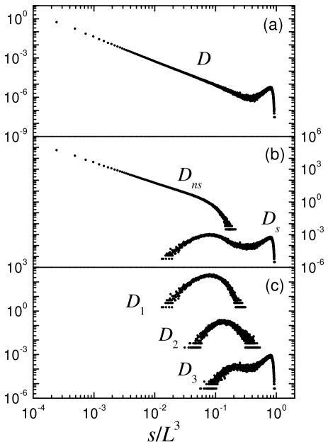
Figure 2: Analysis of the different contributions to $D(s;\sigma,L)$ for $\sigma=2.317$ and $L=16$. Data corresponds to an average of $2\times 10^{5}$ realizations. (a) Full distribution, (b) distribution of spanning avalanches $D_{s}(s;\sigma,L)$; (c) Distributions $D_{1}(s;\sigma,L)$, $D_{2}(s;\sigma,L)$ and $D_{3}(s;\sigma,L)$.

As can be seen the distribution of spanning avalanches $D_{s}(s;\sigma,L)$ is far from simple. It exhibits a multipeak structure caused by the contributions from $D_{1}(s;\sigma,L)$ , $D_{2}(s;\sigma,L)$ and $D_{3}(s;\sigma,L)$ shown in Fig. 2c. Moreover, $D_{3}(s;\sigma,L)$ itself also exhibits two peaks suggesting that the 3d-spanning avalanches may be of two different kinds. We shall denote critical 3d-spanning avalanches (indicated by the subscript $3c$) as those corresponding to the peak on the left and subcritical 3d-spanning avalanches (indicated by the subscript $3-$) as those corresponding to the peak on the right. As will be explained below, the 1d-spanning avalanches, the 2d-spanning avalanches and the critical 3d-spanning avalanches do not exist in the thermodynamic limit except when $\sigma=\sigma_{c}$. This is the reason for having chosen the word “critical” for this kind of 3d spanning avalanche. It will also be shown that, in the thermodynamic limit, subcritical 3d-spanning avalanches only exist for $\sigma\leq\sigma_{c}$. As regards the non-spanning avalanches, they will also be classified into two types at the end of this section, although this separation cannot be deduced from the behaviour in Fig. 2(b).

Fig. 3 shows the evolution of $D_{1}(s,\sigma,L)$, $D_{2}(s,\sigma,L)$ and $D_{3}(s,\sigma,L)$ when $\sigma$ is increased. Note that the right-hand peak of $D_{3}(s;\sigma,L)$ shifts to smaller values of $s$ and becomes flat, indicating that the mean size of these subcritical 3d-spanning avalanches decreases. Moreover, above $\sigma_{c}$ [Fig. 3(d)] this right-hand peak disappears and a peak on the left emerges.

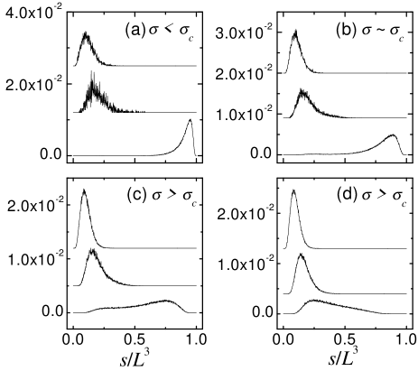
Figure 3: Analysis of the dependence of $D_{1}(s,\sigma;L)$ (top), $D_{2}(s,\sigma;L)$ (middle) and $D_{3}(s,\sigma;L)$ (bottom) with $\sigma$. Data correspond to averages of $2\times 10^{5}$ realizations of a $L=10$ system with (a) $\sigma=1.9$, (b) $\sigma=2.2$, (c) $\sigma=2.5$ and (d) $\sigma=2.8$.

Besides the normalized distributions, it is also interesting to analyze the actual average numbers of spanning avalanches $N_{1}(\sigma,L)$, $N_{2}(\sigma,L)$ and $N_{3}(\sigma,L)$, which also exhibit singular behaviour at $\sigma_{c}$ as shown in Fig. 4.

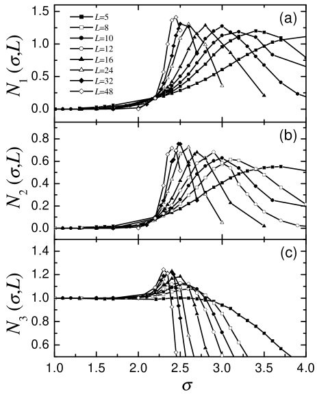
Figure 4: Number of spanning avalanches in 1d (a), 2d (b) and 3d (c) as a function of $\sigma$. The different curves correspond to $L=5,8,10,12,16,24,32$ and $48$ as indicated by the legend. Lines are a guide to the eye.

From the direct extrapolation of the data corresponding to different system sizes to $L\rightarrow\infty$, we can make the following assumptions: in the thermodynamic limit $N_{1}(\sigma)$ and $N_{2}(\sigma)$ will display a $\delta$-function discontinuity at $\sigma_{c}$. $N_{3}(\sigma)$ will display step-like behaviour: for $\sigma<\sigma_{c}$ there is only one 3d-spanning avalanche, for $\sigma>\sigma_{c}$ there are no 3d-spanning avalanches and at $\sigma=\sigma_{c}$ the data supports the assumption that $N_{3}$ will also display a $\delta$-function singularity at the edge of the step function. This reinforces the suggestion that there are two different types of 3d-spanning avalanches: as will be shown, in the thermodynamic limit, the number of subcritical 3d spanning avalanches $N_{3-}$ behaves as a step function, whereas the number of critical avalanches $N_{3c}$ exhibits divergence at $\sigma_{c}$.

The total number of spanning avalanches $N_{s}(\sigma,L)$ and non-spanning avalanches $N_{ns}(\sigma,L)$, are displayed in Figs. 5(a) and 5(b) respectively. $N_{s}(\sigma,L)$ shows, as a result of the divergence of $N_{3c}$, $N_{1}$ and $N_{2}$, a $\delta$-function singularity at $\sigma_{c}$ when $L\rightarrow\infty$ suggesting that the critical point is characterized by the existence of $\infty$ spanning avalanches. We would like to point out that previous studies have not clarified this result for the 3d-GRFIM Perković et al. (1999)

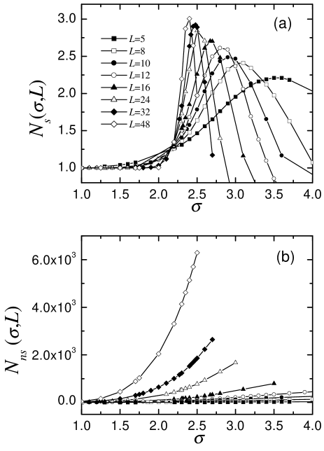
Figure 5: (a) Total number of spanning avalanches $N_{s}(\sigma,L)$ and (b) non-spanning avalanches as a function of $\sigma$ for different system sizes $L$ as indicated by the legend. Lines are a guide to the eye.

The analysis of $N_{ns}$ is more intricate. Fig. 5(b) shows that $N_{ns}(\sigma,L)$ grows with $\sigma$ and $L$. For large amounts of disorder ($\sigma\rightarrow\infty$) one expects that the hysteresis loop consists of a sequence of non-spanning avalanches of size $1$. Therefore, their number will equal $L^{3}$. To reveal this behaviour Fig. 6 shows the dependence of $N_{ns}(\sigma,L)/L^{3}$ as a function of $\sigma$. One expects that these lines tend to $1$ when $\sigma\rightarrow\infty$. Moreover, a closer look reveals that at $\sigma_{c}\simeq 2.21$, there is a contribution to $N_{ns}(\sigma,L)/L^{3}$ which decreases with system size. For low values of $\sigma$ one expects that non-spanning avalanches always exist, except at $\sigma=0$. This last statement can easily be understood by noticing that an approximate lower bound to the number of non-spanning avalanches can be computed by analyzing how many of the spins $S_{i}$ will flip by themselves, independently of their neighbours, due to the fact that the local field $h_{i}$ is either larger than $6$ or smaller than $-6$. This analysis renders $N_{ns}/L^{3}>\Phi_{err}\left(6/\sigma\right)$ where $\Phi_{err}$ is the error function.

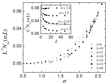
Figure 6: Number of non-spanning avalanches $N_{ns}(\sigma,L)$ divided by $L^{3}$ as a function of $\sigma$ and different system sizes, as indicated by the legend. The inset shows the behaviour of the same quantity as a function of $L$ for different values of $\sigma$. The dashed line indicates the value $N/L^{3}=0.028$ and the continuous line is a fit of the behaviour proposed in equation (26).

From these considerations, we expect that for $L\rightarrow\infty$ the curves in Fig. 6 tend to a certain limiting behaviour which increases smoothly from $0$ to $1$. This can also be appreciated in the inset in Fig. 6, which shows the behaviour of $N_{ns}(\sigma,L)/L^{3}$ as a function of $L$ for four different values of the amount of disorder: $\sigma=1.7$, $\sigma=2.21\simeq\sigma_{c}$, $\sigma=2.5$ and $\sigma=2.7$. The four curves exhibit a tendency to extrapolate to a plateau when $L\rightarrow\infty$. For the case of $\sigma\simeq\sigma_{c}$ an estimation of the extrapolated value is $N_{ns}(\sigma_{c},L)/L^{3}\rightarrow 0.028$.

Consequently, it is necessary to consider the existence of, at least, two kinds of non-spanning avalanches. Those whose number $N_{ns0}$ increases as $L^{3}$ will be denoted as non-critical non-spanning avalanches (with the subscript $ns0$), and those whose number $N_{nsc}$ increases with $L$ with a smaller exponent will be called critical non-spanning avalanches (with the subscript $nsc$). In fact, a log-log plot of $N_{ns}(\sigma_{c},L)/L^{3}-0.028$ versus $L$ provides an estimation for this exponent $N_{nsc}(\sigma_{c},L)\sim 0.085L^{2.02}$.

All the assumptions that have been presented, corresponding to behaviour in the thermodynamic limit, will be confirmed by the finite-size scaling analysis presented in the following sections.

IV Renormalization Group and scaling variables

The basic hypothesis for the analysis of the above results using RG techniques is the existence of a fixed point in the multidimensional space of Hamiltonian parameters. This fixed point sits on a critical surface which extends along all the irrelevant directions. By changing the two tuneable parameters $\sigma$ and $H$, the critical surface can be crossed at the critical point $(\sigma_{c},H_{c})$. As has been explained in the Introduction concerning the analysis of the avalanche number and size distributions, the dependence along the external field direction $H$ has been integrated out. One expects that such integration may distort some of the exponents and the shape of scaling functions, but not the possibility of an RG analysis. This is because the integration range crosses the critical surface where the divergences occur.

For a $L\rightarrow\infty$ system we assume a unique scaling variable $u(\sigma)$ which measures the distance to $\sigma_{c}$. The dependence of $u$ on $\sigma$ should be smooth, but its proper form is unknown S.K.Ma (1973). We will discuss three different possibilities:

1. The standard choice is to use a dimensionless first approximation by expanding $u(\sigma)$ as:

   $$u_{1}=\frac{\sigma-\sigma_{c}}{\sigma_{c}}\;\;.$$ (5)

   Nevertheless, in general, the correct scaling variables may have a different dependence on $\sigma$. For instance, this may be due to the existence of other relevant parameters, such as the external field, which has been integrated out.

2. A second choice is to extend the expansion of $u(\sigma)$ to second order by including a fitting amplitude $A$:

   $$u_{2}=\frac{\sigma-\sigma_{c}}{\sigma_{c}}+A\left(\frac{\sigma-\sigma_{c}}{\sigma_{c}}\right)^{2}\;\;.$$ (6)

3. A third choice, which has been used in previous analyses and may be “phenomenologically” justified is:

   $$u_{3}=\frac{\sigma-\sigma_{c}}{\sigma}\;\;.$$ (7)

   Note that the Taylor expansion of this function is:

   $$u_{3}=\frac{\sigma-\sigma_{c}}{\sigma_{c}}-\left(\frac{\sigma-\sigma_{c}}{\sigma_{c}}\right)^{2}+\left(\frac{\sigma-\sigma_{c}}{\sigma_{c}}\right)^{3}+\cdots\;\;.$$ (8)

Fig. 7, shows the behaviour of the three scaling variables $u_{1}(\sigma)$, $u_{2}(\sigma)$ and $u_{3}(\sigma)$. For the representation of $u_{2}$ we have chosen $A=-0.2$, which is the result that we will fit in the following sections. The three choices are equivalently close enough to the critical point. Nevertheless, the amplitude of the critical zone, where the scaling relations are valid, may be quite different. Since $A<0$, the variable $u_{2}$ cannot be used for $\sigma\gg\sigma_{c}$ since $u_{2}(\sigma)$ shows a maximum at $\sigma=7.735=3.5\sigma_{c}$. A similar problem occurs with $u_{3}$ since, due to its asymptotic behaviour ($u_{3}\rightarrow 1$ for $\sigma\rightarrow\infty$), systems with a large value of $\sigma$ cannot be distinguished one from another.

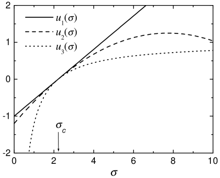
Figure 7: Comparison of the behaviour of the three choices for the scaling variable $u$, discussed in the text. We have used $\sigma_{c}=2.21$.

For the finite system, the magnitudes presented in Table 1, depend on $\sigma$, $L$ and, in the case of the size distributions, on $s$. In order to identify the scaling variables, let us consider a renormalization step of a factor $b$ close to the critical point M.N.Barber (1983); J.Cardy (1996), such that lengths behave as:

$$L_{b}=b^{-1}L\;\;.$$ (9)

(The variables with the $b$ subscript correspond to the renormalized system). We expect that after re-scaling the variable $u$, measuring the distance between $\sigma$ and $\sigma_{c}$ changes as:

$$u_{b}=b^{1/\nu}u\;\;,$$ (10)

which is the standard definition of the exponent $\nu$ which characterizes the divergence of the correlation length when $\sigma\rightarrow\sigma_{c}$. Under the same renormalization step we assume that:

$$s_{b}=b^{-d_{\alpha}}s\;\;.$$ (11)

This latter equation introduces an exponent $d_{\alpha}$ (which has been called $1/\nu\sigma$ by other authors Sethna et al. (1993)) and can be interpreted as the fractal dimension of the avalanches. As mentioned in the previous section, we expect to find different types of avalanches. As will be shown numerically from the scaling plots in the following sections, it is possible to assume that the different types of avalanches behave with the same fractal dimension $d_{\alpha}=d_{f}$, except for subcritical 3d-spanning avalanches (for which $d_{3-}\neq d_{f}$) and non-critical non-spanning avalanches.

Close to the critical point the system exhibits invariance under re-scaling. Therefore, in order to propose a scaling hypothesis of the numbers of avalanches $N_{\alpha}$ and the avalanche size distributions $D_{\alpha}$, it is important to construct combinations of the variables $u$, $L$ and $s$, which remain invariant after renormalization. We find:

$$L_{b}^{1/\nu}u_{b} = L^{1/\nu}u\;\;,$$ (12)

$$L_{b}^{-d_{\alpha}}s_{b} = L^{-d_{\alpha}}s\;\;,$$ (13)

$$s_{b}^{1/\nu d_{\alpha}}u_{b} = s^{1/\nu d_{\alpha}}u\;\;.$$ (14)

Note that these three invariant quantities are not independent since equation (12) corresponds to equation (14) multiplied by equation (13) to the power of $-1/\nu d_{\alpha}$.

V Scaling of the numbers of avalanches $N_{\alpha}(\sigma,L)$

The discussion in the previous section, enables us to propose the following scaling hypothesis:

$$N_{\alpha}(\sigma,L)=L^{\theta_{\alpha}}\tilde{N}_{\alpha}\left(uL^{1/\nu}\right)\;\,.$$ (15)

The exponent $\theta_{\alpha}$ characterizes the divergence of the avalanche numbers at the critical point when $L\rightarrow\infty$. Note that this definition of $\theta_{\alpha}$ (which is the same used in previous works Perković et al. (1999)) is not consistent with the standard finite-size scaling criterion for which the magnitudes grow with exponents divided by $\nu$. M.N.Barber (1983); Goldenfeld (1992); J.Cardy (1996).

As will be shown, the behaviour of the number of 1d-spanning avalanches, 2d-spanning avalanches and critical 3d-spanning avalanches can be described with the same value of $\theta_{1}=\theta_{2}=\theta_{3c}=\theta$, so that:

$$N_{1}(\sigma,L)=L^{\theta}\tilde{N}_{1}\left(uL^{1/\nu}\right)\;\;,$$ (16)

$$N_{2}(\sigma,L)=L^{\theta}\tilde{N}_{2}\left(uL^{1/\nu}\right)\;\;,$$ (17)

$$N_{3c}(\sigma,L)=L^{\theta}\tilde{N}_{3c}\left(uL^{1/\nu}\right)\;\;.$$ (18)

We have tried, without success, to scale the number of critical non-spanning avalanches with the same exponent $\theta$. We therefore need to define a different exponent $\theta_{nsc}$, so that:

$$N_{nsc}(\sigma,L)=L^{\theta_{nsc}}\tilde{N}_{nsc}\left(uL^{1/\nu}\right)\;\;.$$ (19)

As regards the number of $N_{3-}$ avalanches, which is different from zero away from the critical point in the thermodynamic limit, we propose a scaling hypothesis that is compatible with the limiting behaviour at $\sigma=0$ and $\sigma=\infty$. This leads us to the following assumption:

$$N_{3-}(\sigma,L)=\tilde{N}_{3-}\left(uL^{1/\nu}\right)\;\;,$$ (20)

since in the absence of disorder we expect that the hysteresis loop displays a single avalanche of size $L^{3}$, and, consequently the number of avalanches must be $N_{3-}=1$ independent of the value of $L$.

As regards $N_{ns0}$ it has already been discussed that such avalanches will exist in the thermodynamic limit for all values of $\sigma$. Moreover, they are probably not related to critical phenomena at $\sigma_{c}$. For this reason we propose the following non-critical dependence:

$$N_{ns0}(\sigma,L)=L^{3}\tilde{N}_{ns0}(\sigma)\;\;,$$ (21)

In particular, as already mentioned, for large values of disorder ($\sigma\rightarrow+\infty$) these avalanches will be of size $s=1$, and their number will be $N_{ns0}(\infty)=L^{3}$.

It should also be mentioned that the scaling equations (15) admit alternate expressions by extracting the variable $uL^{-1/\nu}$ with the appropriate power so that it cancels out the dependence on $L$:

$$N_{\alpha}(\sigma,L)=|u|^{-\nu\theta_{\alpha}}\tilde{\tilde{N}}_{\alpha}\left(uL^{1/\nu}\right)\;\;.$$ (22)

Nevertheless, such expressions are not very useful for the scaling analysis close to $\sigma_{c}$ since they will display a large statistical error due to the fact that $u\rightarrow 0$ when $\sigma\rightarrow\sigma_{c}$.

Figs. 8 and 9 show the best collapses corresponding to equations (16) and (17) with the three different choices for the variable $u$, explained in section IV. Data corresponding to $L=5,8,10,12,16,24,32$ and $48$ have been used. The quality of the collapses close to $\sigma_{c}$ is quite good in the three cases. The values of the free parameters that optimize each collapse are indicated on the plots. By visual comparison one can see that $u_{2}$ is the best choice since it allows the smaller sizes to collapse too. Of course, this is because the collapses in this case have an extra free-parameter $A$. As regards the quality of the overlaps, no remarkable differences are observed between the choices $u_{1}$ and $u_{3}$. In the following collapses we will use $u_{2}$ with $A=-0.2$. Thus, the best estimations of the free parameters are: $\sigma_{c}=2.21\pm 0.02$, $\nu=1.2\pm 0.1$ and $\theta=0.10\pm 0.02$.

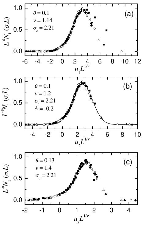
Figure 8: (a) Scaling plot of the number of 1d-spanning avalanches according to equation (16) using $u_{1}$ as the scaling variable. The values of the free parameters for the best collapses are indicated by the legend. Symbols correspond to the sizes indicated in the legend of Fig. 4. (b) Same plot, but using the scaling variable $u_{2}$. Note that in this case there is an extra free parameter. (c) Same plot but using $u_{3}$. The continuous line in (b) shows the fit of a Gaussian function.

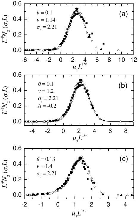
Figure 9: (a) Scaling plot of the number of 2d-spanning avalanches according to equation (17) using $u_{1}$ as the scaling variable. The values of the free parameters for the best collapses are indicated by the legend. Symbols correspond to the sizes indicated in the legend of Fig. 4. (b) Same plot, but using the scaling variable $u_{2}$. Note that in this case there is an extra free parameter. (c) Same plot but using $u_{3}$.The continuous line in (b) shows the fit of a Gaussian function.

The procedure for improving the collapse of the data corresponding to different system sizes, which will be used many times throughout this paper, renders what we will call “the best values” of the free parameters. Error bars represent the estimated range of values for which the collapses are satisfactory. We would like to note that the obtained value of $\sigma_{c}$ (for the three choices of the variable $u$) is slightly higher than the value $\sigma_{c}=2.16\pm 0.03$ proposed in Ref. Perković et al., 1999.

It is interesting to note that the scaling functions ${\tilde{N}}_{1}$ and ${\tilde{N}}_{2}$ can be very well approximated with Gaussian functions. The fits, shown in Figs. 8(b) and 9(b), have three free parameters: the amplitude $a$, the peak position $x$ and the width $w$. The best numerical estimations are: $a_{1}=0.946\pm 0.004$, $x_{1}=2.691\pm 0.008$, $w_{1}=1.293\pm 0.008$, $a_{2}=0.497\pm 0.002$, $x_{2}=2.227\pm 0.007$ and $w_{2}=1.086\pm 0.007$.

From the fact that the scaling functions in Figs. 8(b) and 9(b) are bounded and go exponentially to zero for $u_{2}L^{-1/\nu}\rightarrow\pm\infty$ (as can also be checked from a log-linear plot) one can deduce that, in the thermodynamic limit, 1d-spanning avalanches and 2d-spanning avalanches only exist at $\sigma=\sigma_{c}$. Their numbers increase as $L^{0.10}$ with amplitudes $\tilde{N}_{1}(0)=0.12\pm 0.01$ and $\tilde{N}_{2}(0)=0.07\pm 0.01$. Moreover, the peaks of the scaling functions $\tilde{N}_{1}$ and $\tilde{N_{2}}$ which are displaced from $u_{2}=0$, account for the fact that for a finite system the maximum number of 1d and 2d spanning avalanches occurs for a certain $\sigma_{c}(L)$ which shifts towards $\sigma_{c}$ from above.

As regards the 3d spanning avalanches, according to the previous discussions one must consider the contributions from $N_{3c}$ and $N_{3-}$. From the scaling assumptions (18) and (20) and the last closure relation in Table 2 one can write:

$$N_{3}(\sigma,L)=L^{\theta}\tilde{N}_{3c}\left(uL^{1/\nu}\right)+\tilde{N}_{3-}\left(uL^{1/\nu}\right)\;\;.$$ (23)

This equation indicates that $N_{3}(\sigma,L)$ cannot be collapsed in a straightforward way. We propose here a method to separate the two contributions in equation (23). This method, which we will call double finite-size scaling (DFSS), will be used several times throughout the paper for the analysis of similar equations. By choosing two systems with sizes $L_{1}$ and $L_{2}$ and amounts of disorders $\sigma_{1}$ and $\sigma_{2}$ so that $u(\sigma_{1})L_{1}^{1/\nu}=u(\sigma_{2})L_{2}^{1/\nu}$, one can write:

$$\tilde{N}_{3-}\left(u(\sigma_{1})L_{1}^{1/\nu}\right) = \tilde{N}_{3-}\left(u(\sigma_{2})L_{2}^{1/\nu}\right)=$$

$$= \frac{L_{1}^{-\theta}N_{3}(\sigma_{1},L_{1})-L_{2}^{-\theta}N_{3}(\sigma_{2},L_{2})}{L_{1}^{-\theta}-L_{2}^{-\theta}}$$

$$\tilde{N}_{3c}\left(u(\sigma_{1})L_{1}^{1/\nu}\right) = \tilde{N}_{3c}\left(u(\sigma_{2})L_{2}^{1/\nu}\right)=$$

$$= \frac{N_{3}(\sigma_{1},L_{1})-N_{3}(\sigma_{2},L_{2})}{L_{1}^{\theta}-L_{2}^{\theta}}\;\;.$$

Thus, we can check for the collapse of data corresponding to different pairs of $(L_{1},L_{2})$. From the numerical point of view, the DFSS method works quite well. An analysis of error propagation reveals that the scaling function corresponding to the contribution with a smaller exponent will display more statistical errors.

Fig. 10 shows the results of the DFSS analysis of $N_{3}$ according to equation (23). The different symbols, in this case, indicate the values of $L_{1}$ and $L_{2}$ used for each set of data. Fig. 10(a) corresponds to $\tilde{N}_{3-}(u_{2}L^{1/\nu})$ and Fig. 10(b) corresponds to $\tilde{N}_{3c}(u_{2}L^{1/\nu})$. It should be emphasised that such collapses are obtained without any free parameter. The values of $\theta$, $\sigma_{c}$, $\nu$ and $A$ are taken from the previous collapses of $N_{1}$ and $N_{2}$.

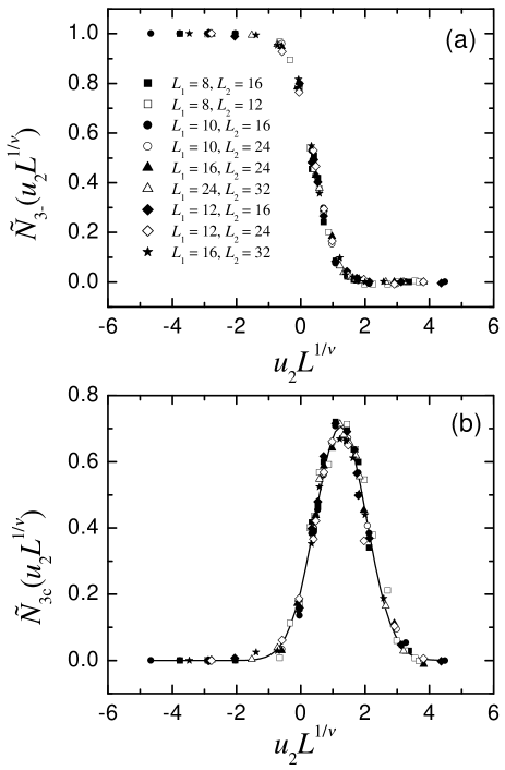
Figure 10: (a) Numerical estimation of $\tilde{N}_{3-}(u_{2}L^{1/\nu})$ and (b) of $\tilde{N}_{3c}(u_{2}L^{1/\nu})$. Data have been obtained according to equations V and V. Symbols, according to the legend, indicate the values of $L_{1}$ and $L_{2}$ used for obtaining each data set. The continuous line in (b) is a fit of a Gaussian function.

Again, from the shape of the scaling functions we can deduce the behaviour in the thermodynamic limit: from the crossing points of the scaling functions with the $u_{2}=0$ axis, we find that $N_{3c}(\sigma_{c},L)=(0.16\pm 0.02)L^{0.10}$ and $N_{3-}(\sigma_{c},L)=0.79\pm 0.02$. As occurred previously with the number of 2d and 1d spanning avalanches, $\tilde{N}_{3c}$ can also be very well approximated with a Gaussian function with amplitude $a_{3c}=0.706\pm 0.005$, peak position $x_{3c}=1.244\pm 0.007$ and width $w_{3c}=0.802\pm 0.009$. The fact that $\tilde{N}_{3c}(u_{2}L^{1/\nu})$ vanishes exponentially for $u_{2}L^{1/\nu}\rightarrow\pm\infty$ confirms that, in the thermodynamic limit, such avalanches only exist at the critical point. Furthermore, from the fact that $\tilde{N}_{3-}$ tends to $1$ and to $0$ exponentially fast when $u_{2}L^{1/\nu}\rightarrow\pm\infty$ we deduce that one subcritical 3d-spanning avalanche will exist for $\sigma<\sigma_{c}$ and there will be none above this value.

To end with the analysis of the number of avalanches, we will separate the two contributions to $N_{ns}$:

$$N_{ns}(\sigma,L)=L^{\theta_{nsc}}\tilde{N}_{nsc}\left(uL^{1/\nu}\right)+L^{3}\tilde{N}_{ns0}\left(\sigma\right)$$ (26)

In this case the DFSS method cannot be applied since $\tilde{N}_{nsc}$ and $\tilde{N}_{ns0}$ depend on different variables. A first check of the validity of this hypothesis has already been presented in section III. The fit of equation (26) to the data corresponding to $\sigma=\sigma_{c}$ $(u=0)$ , shown in the inset of Fig. 6, gives estimations of $\theta_{nsc}\simeq 2.02$ , $\tilde{N}_{ns0}\left(\sigma_{c}\right)=0.028$, and $\tilde{N}_{nsc}\left(0\right)=0.085$. Furthermore, we can also check that the derivative with respect to $\sigma$ behaves as:

$$\frac{1}{L^{3}}\left.\frac{\partial N_{ns}(\sigma,L)}{\partial\sigma}\right|_{\sigma_{c}}=L^{\theta_{nsc}+\frac{1}{\nu}-3}\left(\frac{\tilde{N}_{nsc}^{\prime}(0)}{\sigma_{c}}\right)+\tilde{N}_{ns0}^{\prime}\left(\sigma_{c}\right)$$ (27)

Fig. 11(a) demonstrates that the data (estimated using a two-point derivative formula) is compatible with this behaviour. The line shows the best fit (with two free parameters: $\tilde{N}_{nsc}^{\prime}\left(0\right)$ and $\tilde{N}_{ns0}^{\prime}\left(\sigma_{c}\right)$) of the function (27) with $\theta_{nsc}+1/\nu-3=-0.15$. One obtains $\tilde{N}_{nsc}^{\prime}\left(0\right)=-0.136\pm 0.011$ and $\tilde{N}_{ns0}^{\prime}\left(\sigma_{c}\right)=0.102\pm 0.003$. The good agreement is a test of the dependence with the variables $uL^{1/\nu}$ and $\sigma$ of the functions ${\tilde{N}}_{nsc}$ and ${\tilde{N}}_{ns0}$ respectively. To go further into the analysis of $N_{ns}$, one must provide some extra hypothesis on the shape of the scaling functions. Given the fact that we have found almost a perfect Gaussian dependence of the scaling functions $\tilde{N}_{1}$, $\tilde{N}_{2}$ and $\tilde{N}_{3c}$ one can guess that ${\tilde{N}}_{nsc}$ will also have a Gaussian dependence. By forcing the Gaussian function to satisfy ${\tilde{N}}_{nsc}(0)=0.085$ and the fact that that ${\tilde{N}}_{nsc}^{\prime}(0)=-0.136$ (from previous estimations) we end up with a trial function with a single free parameter that should be enough to satisfactorily scale the data from Fig. 6.

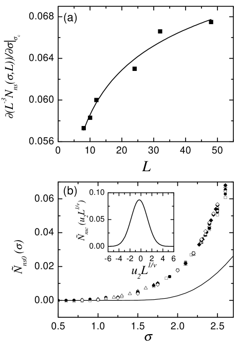
Figure 11: (a) Analysis of the consistency of Eq. (27). The points correspond to numerical data and the line is the best fit (with two free parameters) by fixing the value of $\theta_{nsc}+1/\nu$ to the previous estimations. (b) Scaling plot revealing the behaviour of ${\tilde{N}}_{ns0}(\sigma)$. The continuous line shows the behaviour of the approximate lower bound $\Phi_{err}(6/\sigma)$ estimated from the spins that flip independently of their neighbours. The inset shows the Gaussian function ${\tilde{N}}_{nsc}(u_{2}L^{1/\nu})$ used for the separation of the two contributions to $N_{ns}$.

The best collapse is shown in Fig. 11(b) which corresponds to ${\tilde{N}}_{ns0}(\sigma)$. The function ${\tilde{N}}_{nsc}$ used for the collapse is shown in the inset and corresponds to a Gaussian function with amplitude $a_{nsc}=0.085$, peak position $x_{nsc}=-0.6$ and width $w_{nsc}=1.485$. It is interesting to note that the peak position of this scaling function occurs at a value $u_{2}L^{1/\nu}=x_{nsc}<0$ as opposed to the case of the previous scaling functions ${\tilde{N}}_{1}$, ${\tilde{N}}_{2}$ and ${\tilde{N}}_{3c}$ for which the peak position was at $u_{2}L^{1/\nu}>0$. This indicates that the properties of the $1d$, $2d$ and $3c$ critical avalanches have opposite shifts with finite size $L$ compared to the $nsc$ critical avalanches.

To end with the analysis of the number of non-spanning avalanches it is interesting to compare the function ${\tilde{N}}_{ns0}(\sigma)$ with the approximate lower bound ($\Phi_{err}(6/\sigma)$) discussed in section III, which is represented by a continuous line in Fig. 11(b). The difference between the two curves, which becomes bigger when $\sigma$ increases, is due to the existence of clusters of several spins (not considered in the extremely facile analysis presented here) that flip independently of their neighbours contributing to the number of non-critical non-spanning avalanches.

VI Scaling of the distributions of sizes $D_{\alpha}(s;\sigma,L)$

Close to the critical point there are different ways to express the invariance of the size distributions corresponding to different choices of a pair of invariants among the three exponents proposed in equations (12), (13) and (14). For any generic distribution $D_{\alpha}(s;\sigma,L)$ one can write the following nine generic expressions:

$$D_{\alpha}(s;\sigma,L) = L^{-\tau_{\alpha}d_{\alpha}}\tilde{D}_{\alpha}\left(sL^{-d_{\alpha}},uL^{1/\nu}\right)\;,$$ (28)

$$D_{\alpha}(s;\sigma,L) = L^{-\tau_{\alpha}d_{\alpha}}\bar{D}_{\alpha}\left(s^{1/\nu d_{\alpha}}u,uL^{1/\nu}\right)\;,$$ (29)

$$D_{\alpha}(s;\sigma,L) = L^{-\tau_{\alpha}d_{\alpha}}\hat{D}_{\alpha}\left(s^{1/\nu d_{\alpha}}u,sL^{-d_{\alpha}}\right)\;,$$ (30)

$$D_{\alpha}(s;\sigma,L) = s^{-\tau_{\alpha}}\tilde{\tilde{D}}_{\alpha}\left(sL^{-d_{\alpha}},uL^{1/\nu}\right)\;,$$ (31)

$$D_{\alpha}(s;\sigma,L) = s^{-\tau_{\alpha}}\bar{\bar{D}}_{\alpha}\left(s^{1/\nu d_{\alpha}}u,uL^{1/\nu}\right)\;,$$ (32)

$$D_{\alpha}(s;\sigma,L) = s^{-\tau_{\alpha}}\hat{\hat{D}}_{\alpha}\left(s^{1/\nu d_{\alpha}}u,sL^{-d_{\alpha}}\right)\;,$$ (33)

$$D_{\alpha}(s;\sigma,L) = |u|^{\tau_{\alpha}\nu d_{\alpha}}\tilde{\tilde{\tilde{D}}}_{\alpha}\left(sL^{-d_{\alpha}},uL^{1/\nu}\right)\;,$$ (34)

$$D_{\alpha}(s;\sigma,L) = |u|^{\tau_{\alpha}\nu d_{\alpha}}\bar{\bar{\bar{D}}}_{\alpha}\left(s^{1/\nu d_{\alpha}}u,uL^{1/\nu}\right)\;,$$ (35)

$$D_{\alpha}(s;\sigma,L) = |u|^{\tau_{\alpha}\nu d_{\alpha}}\hat{\hat{\hat{D}}}_{\alpha}\left(s^{1/\nu d_{\alpha}}u,sL^{-d_{\alpha}}\right)\;.$$ (36)

Although we have used the generic index $\alpha$, it is evident that such assumptions can only be proposed for the distributions of avalanches of a single kind, i.e. $D_{1}$, $D_{2}$, $D_{3c}$, $D_{3-}$ and $D_{nsc}$. For the composite distributions $D_{3}$, $D_{s}$, $D_{ns}$ and $D$, one expects mixed behaviour, and concerning $D_{ns0}$ we cannot expect a dependence on $uL^{1/\nu}$. The exponents $\tau_{\alpha}$ could also be different for the different kinds of avalanches, but as will be discussed in the following paragraphs, in all cases $\tau_{\alpha}=1$ except for $\tau_{nsc}$, which will take a larger value.

As argued before, when scaling the numbers of avalanches, the last three expressions (34), (35) and (36) are not very useful for the numerical collapses because they introduce large statistical errors. Moreover, when trying to check the collapses expressed by equations (29) and (32), the two independent variables of the scaling function converge to zero when the critical point is approached. Thus, such a collapse cannot be checked for $u=0$. Therefore, the interesting scaling equations are (28), (30), (31) and (33).

The behaviour of the scaling functions is, in some cases, restricted by the normalization conditions. If scaling holds for the whole range of $s=1,\cdots,L^{3}$, from equation (28), one can write:

$$\sum_{s=1}^{L^{3}}L^{-\tau_{\alpha}d_{\alpha}}\tilde{D}_{\alpha}\left(sL^{-d_{\alpha}},uL^{1/\nu}\right)=1\;.$$ (37)

If $0<d_{\alpha}<3$, by defining a new variable $x=sL^{-d_{\alpha}}$, for large $L$, the above expression is transformed into the following integral:

$$L^{-(\tau_{\alpha}-1)d_{\alpha}}\int_{0}^{\infty}dx\tilde{D}_{\alpha}\left(x,uL^{1/\nu}\right)=1\;.$$ (38)

For those distributions for which the integral converges, it is necessary that $\tau_{\alpha}=1$. We expect that this condition can be applied to the cases of $D_{1}$, $D_{2}$, $D_{3c}$ and $D_{3-}$. In these four cases, as can be seen in Fig. 2(c), the distributions show a marked decay in the two limits of $s\rightarrow 0$ and $s\rightarrow L^{3}$. (Note that the plots have logarithmic scales and that $D_{3c}$ and $D_{3-}$ correspond to the left-hand and right-hand peaks in $D_{3}$ respectively). For the distribution $D_{nsc}$ the exponent $\tau_{nsc}$ can be larger than $1$ since this distribution may extend into the small $s$ region and convergence of the integral in (38) cannot be ensured.

Fig. 12 shows a 3d view of the collapses corresponding to $\tilde{D}_{1}\left(sL^{-d_{f}},u_{2}L^{1/\nu}\right)$. The lines show three cuts of the scaling surface corresponding to $u_{2}L^{1/\nu}=1.21$, $u_{2}L^{1/\nu}=0$ and $u_{2}L^{1/\nu}=-0.56$. The collapses of the curves corresponding to the different sizes are satisfactory within statistical error. The only free parameter in this case is $d_{f}$. The best estimation renders a fractal dimension $d_{f}=2.78\pm 0.05$ for such 1d-spanning avalanches. Similar behaviour is obtained for $\tilde{D}_{2}\left(sL^{-d_{f}},u_{2}L^{1/\nu}\right)$. Although, in principle, we have considered $d_{f}$ as a free parameter, the best collapses are obtained with the same value $d_{f}=2.78$ as that obtained for the 1d-spanning avalanches.

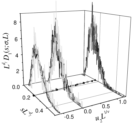
Figure 12: Collapses corresponding to $\tilde{D}_{1}\left(sL^{-d_{f}},u_{2}L^{1/\nu}\right)$. The three cuts of the scaling surface are taken at $u_{2}L^{1/\nu}=1.21$, $u_{2}L^{1/\nu}=0$ and $u_{2}L^{1/\nu}=-0.56$. Note that on each cut we have plotted 5 lines (with different shades of grey) corresponding to $L=8,10,12,16$ and $24$. Symbols on the horizontal plane show the behaviour of the first moment of the distribution according to the legend in figure 4. The line is a guide to the eye.

The analysis of $D_{3c}$ and $D_{3-}$ is more difficult. According to the corresponding distribution relation (see Table 2), and assuming the scaling hypothesis (18), (20) and (28), one can write:

$$N_{3}D_{3}(s;\sigma,L)=$$

$$=L^{\theta-d_{f}}\tilde{N}_{3c}(uL^{1/\nu})\tilde{D}_{3c}\left(sL^{-d_{f}},uL^{1/\nu}\right)+$$

$$+L^{-d_{3-}}\tilde{N}_{3-}(uL^{1/\nu})\tilde{D}_{3-}\left(sL^{-d_{3-}},uL^{1/\nu}\right)\;,$$ (39)

where we have taken into account the fact that for the subcritical 3d-spanning avalanches $\tau_{3d-}=1$ and they have a fractal dimension $d_{3-}$. Although it is possible to conceive a DFSS treatment to separate the two contributions in (39), the hard numerical effort needed as well as the associated statistical uncertainties make it very difficult. In the next section we will show that it is enough to analyze the behaviour of the $k$-moments of the distributions to obtain the critical exponents.

VII Scaling of the $k$-moments of the distributions

Besides the scaling of the entire distributions $D_{\alpha}(s;\sigma,L)$ that exhibit large statistical errors, it is also useful to analyze the behaviour of their $k$-moments. For those distributions for which the integral in Eq.(38) converges (and, therefore, $\tau_{\alpha}=1$), we can check the corresponding scaling functions. By using a similar argument as that used for deriving equation (38), we get:

$$\langle s^{k}\rangle_{\alpha}(\sigma,L)=\sum_{s=1}^{L^{3}}s^{k}D_{\alpha}(s;\sigma,L)=L^{kd_{\alpha}}\Psi_{\alpha}^{k}\left(uL^{1/\nu}\right)\;.$$ (40)

As an example of such collapses, we have indicated the behaviour of the scaled first moment of the distribution $D_{1}(s;\sigma,L)$ on the horizontal plane of Fig. 12. In this case the collapses are obtained without any free parameter.

As will be seen later, it is more convenient to analyze the scaling behaviour of the products $N_{\alpha}\langle s^{k}\rangle_{\alpha}$. By using equations (15) and (40), one gets:

$$N_{\alpha}(\sigma,L)\langle s^{k}\rangle_{\alpha}(\sigma,L)=L^{\theta+kd_{\alpha}}\tilde{N}_{\alpha}\left(uL^{1/\nu}\right)\Psi_{\alpha}^{k}\left(uL^{1/\nu}\right)$$ (41)

Fig. 13 shows the collapses corresponding to the first moment (average size) of $D_{1}$ and $D_{2}$. No free parameters are used in this case. Similar scaling plots can be obtained from the analysis of the second moments with the same set of scaling exponents.

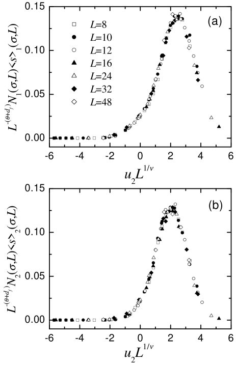
Figure 13: Collapses corresponding to $N_{1}(\sigma,L)\langle s^{k}\rangle_{1}(\sigma,L)$ (a) and $N_{2}(\sigma,L)\langle s^{k}\rangle_{2}(\sigma,L)$ (b). Symbols indicate the system sizes according to the legend.

As regards the scaling of $N_{3}\langle s\rangle_{3}$, multiplying expression (39) by $s$, summing over the whole $s$-range, and imposing condition (37), one obtains:

$$N_{3}\langle s\rangle_{3} = L^{\theta+d_{f}}\tilde{N}_{3c}\left(uL^{1/\nu}\right)\Psi_{3c}^{1}\left(uL^{1/\nu}\right)+$$ (42)

$$+ L^{d_{3-}}\tilde{N}_{3-}\left(uL^{1/\nu}\right)\Psi_{3-}^{1}\left(uL^{1/\nu}\right)\;.$$

This equation can be separated by a DFSS analysis. Figs. 14(a) and 14(b) show the collapses corresponding to $\tilde{N}_{3c}\Psi_{3c}^{1}$ and $\tilde{N}_{3-}\Psi_{3-}^{1}$ respectively. The only free parameter in this scaling plot is the fractal dimension of the subcritical 3d-spanning avalanches. The best value is $d_{3-}=2.98\pm 0.02$. Note that the shape of the scaling function in Fig. 14(b) indicates that, in the thermodynamic limit, the critical 3d-spanning avalanches only contribute to the first-moment for $\sigma=\sigma_{c}$

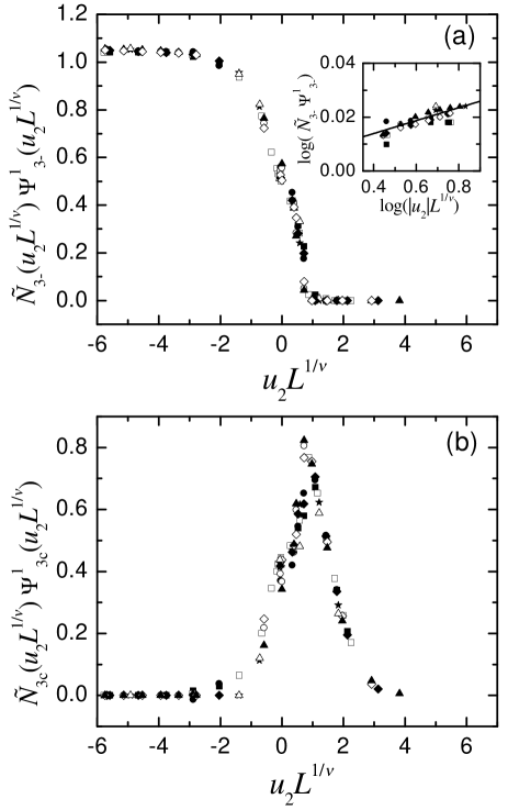
Figure 14: Collapses corresponding to $\tilde{N}_{3-}(uL^{1/\nu})\Psi_{3-}^{1}(u_{2}L^{1/\nu})$ (a) and $\tilde{N}_{3c}(u_{2}L^{1/\nu})\Psi_{3c}^{1}u_{2}L^{1/\nu})$ (b). Symbols indicate the values of $L_{1}$ and $L_{2}$ used for the DFSS analysis according to the legend in Fig. 10. The inset in (a) reveals the power-law behaviour $\tilde{N}_{3-}\Psi_{3-}^{1}\sim(|u_{2}|L^{1/\nu})^{\beta_{3-}}$ with $\beta_{3-}=0.024$.

On the other hand, the shape of the scaling function in Fig. 14(a) indicates that, in the thermodynamic limit, the subcritical 3d-spanning avalanches may contribute to the first moment in the whole $u_{2}<0$ range. Note that, as revealed by the inset in Fig. 14(a), the behaviour in the region of negative values of $u_{2}L^{1/\nu}$ is $\tilde{N}_{3-}\Psi_{3-}^{1}\sim(|u_{2}|L^{1/\nu})^{\beta_{3-}}$ with $\beta_{3-}=0.024\pm 0.012$. This numerical value is compatible with the equation:

$$\beta_{3-}=\nu(3-d_{3-})$$ (43)

This hyperscaling relation, when introduced into equation (42), results in a second term that grows with $L^{3}$. As will be analyzed in the next section, such a term will be responsible for the order parameter behaviour in the thermodynamic limit.

The analysis of the moments of the non-spanning avalanches presents extra difficulties, as occurred in the analysis of their number. The expected behaviour is:

$$N_{ns}(\sigma,L)\langle s^{k}\rangle_{ns}(\sigma,L)=$$

$$=L^{\theta_{nsc}+(1+k-\tau_{nsc})d_{nsc}}\tilde{N}_{nsc}(uL^{1/\nu})\Psi_{nsc}^{k}\left(uL^{1/\nu}\right)+$$

$$+L^{3}\tilde{N}_{ns0}(\sigma)\Psi_{ns0}^{k}\left(\sigma\right)\;.$$ (44)

As explained previously, the DFSS cannot be applied, given the different dependence on $uL^{1/\nu}$ and $\sigma$ of the two terms in (44). The possibility of using a trial function is, now, more difficult since we cannot make a straighforward hypothesis on the shape of $\Psi_{nsc}^{k}$. In order to fit the value of $\tau_{nsc}$ and $d_{nsc}$ we can analyze the dependence of the $k$-moment (for $k=2$ and $k=3$) and its derivatives with respect to $\sigma$ at $\sigma=\sigma_{c}$ ($u=0$). Data is shown in Fig. 15(a) and Fig. 15(b) with log-log scales. The almost perfect power-law behaviour for different values of $k$ and for the derivatives, indicates that the second term in (44) plays no role in $\sigma_{c}$. This is because the exponent of the first term is much larger than 3. Indeed, the best fits are obtained with $d_{nsc}=d_{f}=2.78\pm 0.05$ and $\tau_{nsc}=1.65\pm 0.02$ which render large values of the exponent of the first term ($>5.8$). Similar fits can be obtained from higher moments with the same values of the exponents $d_{nsc}$ and $\tau_{nsc}$.

VIII Magnetization discontinuity

In this section we discuss the behaviour of the discontinuity $\Delta m$ in the magnetization of the hysteresis loop. We would like it to behave as an order parameter. For large systems, it is clear that only spanning avalanches may produce a discontinuity in the magnetization. We can evaluate the total average magnetization jump $\Delta m_{s}$ due to the contribution of all the spanning avalanches ($1d$, $2d$, $3c$ and $3-$).

$$\Delta m_{s}=\frac{2}{L^{3}}N_{s}\langle s\rangle_{s}\;.$$ (45)

Fig. 16(a) shows the behaviour of $\Delta m_{s}$ versus $\sigma$ for different system sizes. According to the scaling analysis in the previous section, $\Delta m_{s}$ will behave as:

$$\Delta m_{s}(\sigma,L) = 2\left\{L^{\theta+d_{f}-3}\left[{\tilde{N}}_{1}(uL^{1/\nu})\Psi_{1}\left(uL^{1/\nu}\right)+{\tilde{N}}_{2}\left(uL^{1/\nu}\right)\Psi_{2}\left(uL^{1/\nu}\right)+{\tilde{N}}_{3c}\left(uL^{1/\nu}\right)\Psi_{3c}\left(uL^{1/\nu}\right)\right]\right.$$ (46)

$$+ \left.L^{d_{3-}-3}{\tilde{N}}_{3-}\left(uL^{1/\nu}\right)\Psi_{3-}\left(uL^{1/\nu}\right)\right\}\;.$$

This equation tells us that $\Delta m_{s}$ will display a mixed scaling behaviour. The first term in (46) accounts for the contributions of the 1d-spanning, 2d-spanning and critical 3d-spanning avalanches. We can define an exponent $\beta_{c}$ so that:

$$\frac{\beta_{c}}{\nu}\equiv-\left(\theta+d_{f}-3\right)\;\;.$$ (47)

Figure 15: (a) Behaviour of $N_{ns}(\sigma_{c},L)\langle s^{k}\rangle_{ns}(\sigma_{c},L)$ as a function of L for $k=1$ and $k=2$ in log-log scale. (b) Behaviour of the derivative with respect to $\sigma$ of the same two magnitudes. In both cases, the lines show the best fits of Eq.44 and its derivative at $\sigma=\sigma_{c}$.

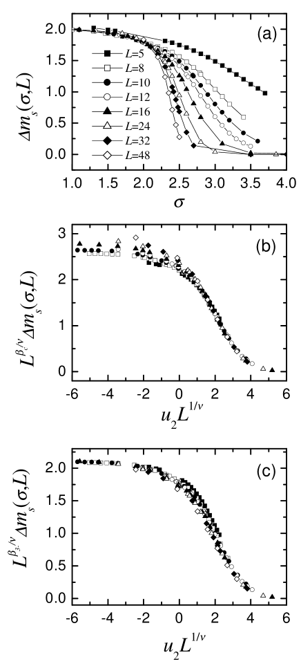
Figure 16: (a) Behaviour of the total contribution of the spanning avalanches to the magnetization jump as a function of $\sigma$. The inset reveals the crossing behaviour at $\sigma<\sigma_{c}$. (b) Scaling of $\Delta m_{s}$ by considering the 1d, 2d, and the critical 3d-spanning avalanches. Note the lack of collapse for the region $u_{2}L^{1/\nu}\lesssim 0$. (c) Scaling of $\Delta m_{s}$ by considering the subcritical 3d-spanning avalanches. Note the lack of collapse for the region $u_{2}L^{1/\nu}\sim 0$. Symbols indicate the system sizes according to the legend.

This relation is the same relation that other authors have called “violation of hyperscaling” A.Maritan et al. (1994); Dahmen and J.P.Sethna (1996); Perković et al. (1999). From our best estimations of $\theta$, $\nu$ and $d_{f}$, we obtain $\beta_{c}=0.15\pm 0.08$.

At this point, it is interesting to compare equations (43) and (47.) We would like to note that we could also have introduced an exponent $\theta^{\prime}$ that would transform Eq. (43) into an equation similar to (47). Nevertheless, the quality of the scalings of the numbers of 3d-spanning avalanches in Fig. 10 shows that such an exponent $\theta^{\prime}$ is either zero or very small. Moreover, an analysis of the behaviour of ${\tilde{N}}_{3-}$ for $uL^{1/\nu}\rightarrow-\infty$ reveals an exponential drift versus ${\tilde{N}}_{3-}=1$ which reinforces the idea that there is no need for an hyperscaling exponent $\theta^{\prime}$. Note that a value $\theta^{\prime}>0$ implies that the number of subcritical 3d-spanning avalanches ($3-$) will be infinite, in the thermodynamic limit. On the other hand, our assumption that $\theta^{\prime}=0$ indicates that $N_{3-}$ behaves as a step function in the thermodynamic limit.

By inserting equations (43) and (47) into (46) one can easily read the mixed scaling behaviour of $\Delta m_{s}$:

$$\Delta m_{s}(\sigma,L)\propto L^{-\beta_{c}/\nu}\Phi(uL^{1/\nu})+L^{-\beta_{3-}/\nu}\Phi^{\prime}(uL^{1/\nu})$$ (48)

where, $\beta_{c}/\nu=0.12$ and $\beta_{3-}/\nu=0.02$. $\Phi$ is a scaling function with a peaked shape (it corresponds to the sum of the scaling functions in Figs. 13(a), 13(b) and 14(b)) and $\Phi^{\prime}$ is twice the scaling function in Fig. 14(b). Consequently, in the thermodynamic limit, only the second term associated to the subcritical 3d-spanning avalanches will contribute to the magnetization jump (order parameter). For finite systems, the first term may affect the scaling of the data close to $\sigma_{c}$ given the peaked shape of $\Phi$.

This behaviour can be observed in Figs. 16(b) and 16(c), where the two possible scalings show the breakdown of the collapse for $u_{2}L^{1/\nu}<0$ when using the exponent $\beta_{c}/\nu$ and the breakdown of the collapse for $u_{2}L^{1/\nu}\simeq 0$ when using the exponent $\beta_{3-}/\nu$. The larger the system, the better will be the data collapse in Fig. 16(c) and the worse will be the collapse in Fig. 16(b).

IX Discussion

Table 3 shows a summary of the exponents that characterize the avalanche numbers and distributions obtained from our numerical simulations. We would like to point out that such exponents are independent of $\sigma$ and $L$ in a very large region around the critical point both for $\sigma>\sigma_{c}$ and $\sigma<\sigma_{c}$ simultaneously. Such an achievement has not been possible in previous analyses, even with larger system sizes. The reason is that some of the contributions we have identified (namely $3-$ and $ns0$), which reduce finite size effects, were previously neglected.

exponent	best value	values in Ref. Perković et al.,1999
$\nu$	$1.2\pm 0.1$	$1.41\pm 0.17$
$\theta$	$0.10\pm 0.02$	$0.15\pm 0.15$
$\theta_{nsc}$	$2.02\pm 0.04$
$d_{f}$	$2.78\pm 0.05$	$2.98\pm 0.43$ ($=1/\sigma\nu$)
$d_{3-}$	$2.98\pm 0.02$
$\tau_{nsc}$	$1.65\pm 0.02$
$\beta_{c}$	$0.15\pm 0.08$
$\beta_{3-}$	$0.024\pm 0.012$	$0.035\pm 0.032$ ($=\beta$)

Table 3: Summary of the values of the exponents obtained from the simulations in this work. We have indicated the names of the exponents from Ref. Perković et al., 1999, whose definition does not exactly correspond to our nomenclature between parentheses.

In Table 3 we also indicate previous estimations of the exponents found in the literature Perković et al. (1999). The comparison is quite satisfactory. Let us analyze the eight exponents:

• Although the value of $\nu$ does not fall within the error bars in Ref. Perković et al., 1999, we have already argued that the exact definition of the scaling variable $u$ used for the collapses may introduce some deviations in this value. By using $u_{1}$ we obtain $\nu=1.14$ and using $u_{3}$ we obtain $\nu=1.4$.

• As regards $\theta$ our value is in agreement with the value previously reported Perković et al. (1999) (We would like to note that in Ref. Perković et al., 1999, the authors also report a value of $0.015\pm 0.015$ probably due to a misprint). The fact that this exponent is non-zero implies that there are infinite spanning avalanches at the critical point in the thermodynamic limit.

• As regards $\theta_{nsc}$, to our knowledge there are no previous finite-size scaling analyses of the number of non-spanning avalanches.

• Concerning $d_{f}$ and $d_{3-}$, the numerical values are consistent with the value $d_{f}=2.98\pm 0.43$ estimated previously Perković et al. (1995). We shall note that this previous estimation was obtained from the analysis of the distributions of non-spanning avalanches. It should therefore correspond to our $d_{f}$ and not to our $d_{3-}$ (which corresponds to the subcritical 3d-spanning avalanches). Note also that the difference between $d_{f}$ and $d_{3-}$ suggests that there might be real physical differences between such two kinds of avalanches. The possibility of distinguishing them in the numerical simulation will be studied in a future work.

• The exponent $\tau_{nsc}$, according to our definitions, describes the scaling behaviour of the distribution of critical non-spanning avalanches. Previous measurements of a similar exponent, have analyzed $N_{ns}$ without distinguishing between critical (nsc) and non-critical (ns0) non-spanning avalanches and have not considered the fact that the system is finite. We can estimate what the value of an effective exponent $\tau_{eff}$ will be for the distribution of non-spanning avalanches for very large systems. From equation (44), taking $k>1$, and large values of $L$, only the first term in the sum survives, so that:

  $$N_{ns}(\sigma)\langle s^{k}\rangle_{ns}(\sigma)=$$

  $$=L^{\theta_{nsc}+(1+k-\tau_{nsc})d_{f}}\tilde{N}_{nsc}\left(uL^{1/\nu}\right)\Psi_{nsc}^{k}\left(uL^{1/\nu}\right).$$

  On the other hand, in the same limit, the analysis of equation (26) renders:

  $$N_{ns}(\sigma)=L^{3}\tilde{N}_{ns0}\left(\sigma\right)\;.$$ (50)

  Combining the last two equations, we get an estimation for the pseudo-scaling behaviour of the $k$-moment of the non-spanning avalanches:

  $$\langle s^{k}\rangle_{ns}(\sigma)=$$

  $$=L^{\theta_{nsc}+(1+k-\tau_{nsc})d_{f}-3}\frac{\tilde{N}_{nsc}(uL^{1/\nu})}{\tilde{N}_{ns0}(\sigma)}\Psi_{nsc}^{k}\left(uL^{1/\nu}\right)\;.$$

  If one approximates $\tilde{N}_{ns0}(\sigma)$ by $\tilde{N}_{ns0}(\sigma_{c})$ and imposes $\langle s^{k}\rangle_{ns}\sim L^{-(\tau_{eff}-k-1)d_{f}}{\cal S}^{k}(uL^{1/\nu})$ it is possible to deduce that the effective exponent is $\tau_{eff}=\tau_{nsc}+\left(3-\theta_{nsc}\right)/d_{f}$. From our numerical estimations of the different exponents in Table 3, one obtains $\tau_{eff}=2.00\pm 0.06$. This value is in very good agreement with the value $\tau_{eff}=2.03\pm 0.03$ found previously Perković et al. (1999). Nevertheless, we would like to point out that according to our analysis, such an exponent is not a real critical exponent and, therefore, will depend on $\sigma$ for finite systems as has been found previously O.Perković et al. (1996).

• As regards the values of $\beta_{c}$ and $\beta_{3-}$ we would like to note that previous analyses have not identified the two contributions to $\Delta m_{s}$. It is therefore not strange that different values have been obtained previously: $0.17\pm 0.07$ Sethna et al. (1993), $0.0\pm 0.43$ Dahmen and J.P.Sethna (1996), $0.035\pm 0.028$ Perković et al. (1999). The larger the system, the closer the effective exponent becomes to $\beta_{3-}$.

Finally, it is interesting to compare the behaviour of spanning avalanches, with the problem of percolation Stauffer and A.Aharony (1994). In percolation, the number of percolating clusters behaves as a step function, in the thermodynamic limit for $d<6$, exactly as $N_{3-}$. The order parameter is, in this case, the probability for a site to belong to the percolating cluster. However, this is precisely what we are evaluating by the function $N_{3-}\langle s\rangle_{3-}/L^{3}$ which is the second term in (46) and is the only relevant term in the thermodynamic limit. As occurs in percolation, the hyperscaling relation (43) between $\beta_{3-}$, $\nu$ and $d_{3-}$ is fulfilled since only one infinite avalanche contributes to the order parameter for $\sigma\rightarrow\sigma_{c}$ from below. Moreover, in the percolation problem for $d>6$ de Arcangelis (1987), the number of percolating clusters exhibits, besides the step function, an extra $\delta$-function singularity at the percolation threshold. In our case (3d-GRFIM) we also have such a contribution at $\sigma=\sigma_{c}$, which we have identified as 1d, 2d and critical 3d-spanning avalanches [the first term in (46)]. The existence of such an infinite number of avalanches exactly at $\sigma_{c}$ (the number of which grows as $L^{\theta}$) implies the breakdown of the hyperscaling relation $\beta_{c}=\nu[3-(\theta+d_{f})]$.

X Summary and conclusions

In this paper we have presented finite-size scaling analysis of the avalanche numbers and avalanche distributions in the 3d-GRFIM with metastable dynamics. After proposing a number of plausible scaling hypotheses, we have confirmed them by obtaining very good collapses of the numerical data corresponding to systems with sizes up to $L=48$.

The first result is that, in order to obtain a good description of the numerical data, one needs to distinguish between different kinds of avalanches which behave differently when the system size is increased. Avalanches are classified as being: non-spanning, 1d-spanning, 2d-spanning or 3d-spanning. Furthermore, we have shown that the 3d-spanning avalanches must be separated into two classes: subcritical 3d-spanning avalanches with fractal dimension $d_{3-}=2.98$ and critical 3d-spanning avalanches with fractal dimension $d_{f}=2.78$, as the $1d-$ and $2d-$spanning avalanches. Non-spanning avalanches occur for the whole range of $\sigma$. We have also proposed a separation between critical non-spanning avalanches and non-critical non-spanning avalanches in order to obtain good finite-size scaling collapses. The non-critical non-spanning avalanches are those whose size is independent of the system size and whose number scales as $L^{3}$. The critical non-spanning avalanches also have a fractal dimension $d_{f}=2.78$.

The second important result, is the scenario for the behaviour in the thermodynamic limit: below the critical point, there is only one subcritical 3d-spanning avalanche, which is responsible for the discontinuity of the hysteresis loop. Furthermore, at the critical point there are an infinite number of 1d-, 2d-, and 3d- critical spanning avalanches.

For finite systems, the six different kinds of avalanches can exist above, exactly at and below $\sigma_{c}$. The finite-size scaling analysis we have performed has also enabled us to compare different scaling variables $u$, which measure the distance between the amount of disorder in the system $\sigma$ and the critical amount of disorder $\sigma_{c}$. The best collapses are obtained using the variable $u_{2}=(\sigma-\sigma_{c})/\sigma_{c}+A\left[(\sigma-\sigma_{c})/\sigma_{c}\right]^{2}$ with $A=-0.2$.

So far the analysis presented in this paper, is restricted to the analysis of the numbers and distributions of avalanches integrated along half a hysteresis loop. Our analysis of the average magnetization discontinuity $\Delta m$ starts from the hypothesis that only spanning avalanches may contribute to such a discontinuity. However, as a future study, we suggest that the measurement of correlations in the sequence of avalanches and the analysis of non-integrated distributions, may reveal details of the singular behaviour at the critical field $H_{c}$. For instance, non-spanning avalanches could show a tendency to accumulate in $H_{c}$, in the thermodynamic limit. This could change some of the conclusions reached in this work.

As a final general conclusion we have shown that it is not necessary to simulate very large system sizes to estimate the critical exponents for this model. In order to identify the different kinds of avalanches it may even be better to analyze small systems with larger statistics.

XI Acknowledgements

We acknowledge fruitful discussions with Ll.Mañosa and A.Planes. We acknowledge an anonymous referee for helping us to understand the difference between the present method of counting avalanches and the method used in previous works. This work has received financial support from CICyT (Spain), project MAT2001-3251 and CIRIT (Catalonia) , project 2000SGR00025. F.J. P. also acknowledges financial support from DGICyT.

References

- Vives and Planes (1994) E. Vives and A. Planes, Phys. Rev. B 50, 3839 (1994).
- Carrillo et al. (1998) L. Carrillo, Ll.Mañosa, J. Ortín, A. Planes, and E.Vives, Phys. Rev. Lett. 81, 1889 (1998).
- D.Sornette (2000) D.Sornette, Critical Phenomena in Natural Sciences, Springer Series in Synergetics (Springer Verlag, 2000).
- P.J.Cote and L.V.Meisel (1991) P.J.Cote and L.V.Meisel, Phys. Rev. Lett. 67, 1334 (1991).
- M.P.Lilly et al. (1993) M.P.Lilly, P.T.Finley, and R.B.Hallock, Phys. Rev. Lett. 71, 4186 (1993).
- W.Wu and P.W.Adams (1995) W.Wu and P.W.Adams, Phys. Rev. Lett 74, 610 (1995).
- Vives et al. (1994) E. Vives, J. Ortín, L. Mañosa, I. Ràfols, R. Pérez-Magrané, and A. Planes, Phys. Rev. Lett. 72, 1694 (1994).
- Sethna et al. (1993) J. P. Sethna, K. Dahmen, S. Kartha, J. A. Krumhansl, B. W. Roberts, and J. D. Shore, Phys. Rev. Lett. 70, 3347 (1993).
- Dahmen and J.P.Sethna (1993) K. A. Dahmen and J.P.Sethna, Phys. Rev. Lett. 71, 3222 (1993).
- Perković et al. (1995) O. Perković, K. A. Dahmen, and J.P.Sethna, Phys. Rev. Lett 75, 4528 (1995).
- Dahmen and J.P.Sethna (1996) K. A. Dahmen and J.P.Sethna, Phys. Rev. B 53, 14872 (1996).
- Tadić (1996) B. Tadić, Phys. Rev. Lett. 77, 3843 (1996).
- Perković et al. (1999) O. Perković, K. A. Dahmen, and J.P.Sethna, Phys. Rev. B 59, 6106 (1999).
- Kuntz et al. (1999) M. C. Kuntz, O. Perković, K. A. Dahmen, B. Roberts, and J.P.Sethna, Computing in Science & Engineering July/August, 73 (1999).
- J.H.Carpenter and K.A.Dahmen (2002) J.H.Carpenter and K.A.Dahmen, cond-mat/0205021 (2002).
- O.Perković et al. (1996) O.Perković, K.A.Dahmen, and J.P.Sethna, cond-mat/9609072 (1996).
- B.Tadić and U.Nowak (2000) B.Tadić and U.Nowak, Phys. Rev. E 61, 4610 (2000).
- S.K.Ma (1973) S.K.Ma, Rev. Mod. Phys. 45, 589 (1973).
- M.N.Barber (1983) M.N.Barber, Finite Size Scaling, vol. 8 of Phase Transitions and Critical Phenomena (Academic Press, London, 1983).
- J.Cardy (1996) J.Cardy, Scaling and Renormalization in Statistical Physics (Cambridge University Press, 1996).
- Goldenfeld (1992) N. Goldenfeld, Lectures on Phase Transitions and the Renormalization Group (Addison-Wesley, Reading, MA, 1992).
- A.Maritan et al. (1994) A.Maritan, M.Cieplak, M.R.Swift, and J.R.Banavar, Phys. Rev. Lett. 72, 946 (1994).
- Stauffer and A.Aharony (1994) J. Stauffer and A.Aharony, Introduction to percolation theory (Taylor and Francis, 1994), 2nd ed.
- de Arcangelis (1987) L. de Arcangelis, J. Phys. A 20, 3057 (1987).