Global climate models violate scaling of the observed atmospheric variability

Abstract

We test the scaling performance of seven leading global climate models by using detrended fluctuation analysis. We analyse temperature records of six representative sites around the globe simulated by the models, for two different scenarios: (i) with greenhouse gas forcing only and (ii) with greenhouse gas plus aerosol forcing. We find that the simulated records for both scenarios fail to reproduce the universal scaling behavior of the observed records, and display wide performance differences. The deviations from the scaling behavior are more pronounced in the first scenario, where also the trends are clearly overestimated.

Confidence in the simulation and prediction skills of global climate models (coupled atmosphere-ocean general circulation models 1 ; Has AOGCMs) is a crucial precondition for formulating climate protection policies. The models provide numerical solutions of the Navier–Stokes equations devised for simulating meso-scale to large-scale atmospheric and oceanic dynamics. In addition to the explicitly resolved scales of motions, the models also contain parameterization schemes representing the so-called subgrid-scale processes, such as radiative transfer, turbulent mixing, boundary layer processes, cumulus convection, precipitation, and gravity wave drag. A radiative transfer scheme, for example, is necessary for simulating the role of various greenhouse gases such as CO₂ and the effect of aerosol particles. The differences among the models usually lie in the selection of the numerical methods employed, the choice of the spatial resolution FN1 , and the subgrid-scale parameters.

Two scenarios (apart from a control run with fixed CO₂ content) have been studied by the models, and the results are available from the IPCC Data Distribution Center 26 . In the first scenario, one considers only the effect of greenhouse gas forcing. The amount of greenhouse gases is taken from the observations until 1990 and then increased at a rate of 1% per year. In the second scenario, also the effect of aerosols (mainly sulphates) in the atmosphere is taken into account. Only direct sulphate forcing is considered; until 1990, the sulphate concentrations are taken from historical measurements, and are increased linearly afterwards. The effect of sulphates is to mitigate and partially offset the greenhouse gas warming. Although this scenario represents an important step towards comprehensive climate simulation, it introduces new uncertainties — regarding the distributions of natural and anthropogenic aerosols and, in particular, regarding indirect effects on the radiation balance through cloud cover modification, etc. WGI .

All of the models are capable, to varying extents, to reproduce the current mean state of the atmosphere fn2 . The models have been validated by comparing to historical data and by intercomparison of the models 3 ; 9 . The efforts have been restricted to traditional time series analysis which generally assumes that the statistical properties of a signal remain the same throughout the entire period. This assumption of stationarity, however, is certainly not valid for climate records due to imposed effects such as global or urban warming.

In our evaluation of the models, we apply detrended fluctuation analysis (DFA) 11 ; 13 which can distinguish between trends and correlations and thus reveal trends as well as long term correlations very often masked by nonstationarities. Recently, Koscielny-Bunde et al. 2 ; 14 applied DFA and wavelet techniques (see, e. g. 12 ) to investigate temporal correlations in the atmospheric variability. Considering maximum daily temperature records of various stations around the globe, they analyzed the temperature variations from their average values and found that the persistence, characterized by the correlation $C(s)$ between temperature variations separated by $s$ days, decays with a power law,

$$C(s)\sim s^{-\gamma},$$ (1)

with roughly the same correlation exponent $\gamma\cong 0.7$ for all stations considered. The range of this persistence law exceeds ten years, and there is no evidence for a breakdown of the law at even larger time scales. Indications for the long term persistence through spectral analysis have also been obtained 15 ; Talkner . Since the persistence scaling law appears to be universal, i. e. independent of the location and climatic zone of the stations, we use it in the following for assessing the performance of the AOGCMs.

For the test, we consider monthly averages of the daily maximum temperature from seven AOGCMs: GFDL-R15-a (Princeton), CSIRO-Mk2 (Melbourne), ECHAM4/OPYC3 (Hamburg), HADCM3 (Bracknell, UK), CGCM1 (Victoria, Canada), CCSR/NIES (Tokyo), NCAR PCM (Boulder, USA) (see 26 for details). We extracted the data for six representative sites around the globe (Prague, Kasan, Seoul, Luling/Texas, Vancouver, and Melbourne). For each model and each scenario, we selected the temperature records of the 4 grid points closest to each site, and bilinearly interpolated the data to the location of the site. We analyze both scenarios but we focus more on the better established first scenario.

We analyze for each site the variations $\Delta T_{i}$ of the monthly temperatures $T_{i}$ from the respective monthly mean temperature $\overline{T_{i}}$ that has been obtained by averaging over all years in the record. Quantitatively, persistence in $\Delta T_{i}$ can be characterized by the (auto) correlation function, $C(s)\equiv\langle\Delta T_{i}\Delta T_{i+s}\rangle=(1/(N-s))\sum_{i=1}^{N-s}\Delta T_{i}\Delta T_{i+s},$ where $N$ is the total number of months in the record. A direct calculation of $C(s)$ is hindered by the level of noise present in the finite temperature series, and by possible nonstationarities in the data. Following Refs. 28 and 29 , we do not calculate $C(s)$ directly, but instead study the fluctuations in the temperature “profile” $Y_{n}=\sum_{i=1}^{n}\Delta T_{i}$. To this end, we divide the profile into (nonoverlapping) segments of length $s$ and determine the squared fluctuations of the profile (specified below) in each segment. The mean square fluctuations, averaged over all segments of length $s$, are related to the correlation function $C(s)$ (see below). In our test, we employ a hierarchy of methods that differ in the way the fluctuations are measured and possible nonstationarities are eliminated (for a detailed description of the methods we refer to 13 ) :

1. In the (standard) fluctuation analysis (FA), we calculate the difference of the profile at both ends of each segment. The square of this difference represents the square of the fluctuations in each segment.

2. In the “first order detrended fluctuation analysis” (DFA1), we determine in each segment the best linear fit of the profile. The standard deviation of the profile from this straight line represents the square of the fluctuations in each segment.

3. More generally, in the “$n$th order DFA” (DFA$n$), we determine in each segment the best $n$th-order polynomial fit of the profile. Again, the standard deviation of the profile from these polynomials represents the square of the fluctuations in each segment.

The fluctuation function $F(s)$ is the root mean square of the fluctuations in all segments. For the relevant case of long-term power-law correlations given by Eq. 1, with $0<\gamma<1$, the fluctuation function $F(s)$ increases according to a power law 30 ,

$$F(s)\sim s^{\alpha},\qquad\alpha=1-\frac{\gamma}{2}.$$

For uncorrelated data (as well as for short-range correlations represented by $\gamma\geq 1$ or exponentially decaying correlation functions), we have $\alpha=\frac{1}{2}$. For long term correlations we have $\alpha>\frac{1}{2}$.

Figure 1: Results of FA and DFA for the monthly averages of the daily maximum temperature of Luling (a–d) and Kasan (e–h). In each panel, the curves from top to bottom represent the fluctuation function $F(s)$ obtained from FA ($\triangle$) and DFA1–DFA5 (o), respectively. Full symbols represent past data and open symbols are for the entire simulation period. The scale of $F(s)$ is arbitrary. The maximum value of $s$ is $1/4$ of the length of the considered record. The two lines shown at the bottom are theoretical lines with slope 0.65 (upper line) and 0.5 (lower line). Note that FA (which does not remove trends) overestimates the fluctuation exponent as can be seen when comparing to DFA. As seen in the figures, the differences in the exponents obtained by DFA3 and higher orders of DFA are negligible, which means that in DFA3 all trends are removed from the data. For this reason, when focusing on the correlation exponent, it is sufficient to use DFA3 (as done in Figure 2).

By definition, the FA does not eliminate trends, similar to the Hurst method and the conventional spectral analysis 31 . In contrast, DFAn eliminates polynomial trends of order $n-1$ in the original data. Thus, from the comparison of the various fluctuation functions $F(s)$ obtained by these methods, we can learn both about long term correlations and types of trends, which cannot be achieved by the conventional spectral analysis.

Figure 2: Results of DFA3 applied to the monthly averages of the daily maximum temperature of (a) real data and (b–h) simulated data (for scenario (i)) at the respective geographical positions of Prague (Pr), Melbourne (Me), Luling (Lu), Seoul (Se), Kasan (Ka) and Vancouver (Va), for the seven AOGCMs considered. In each panel, curves from top to bottom represent the result for the six sites. For better evaluation of the models, $F(s)$ is divided by $s^{0.5}$. The scale of $F(s)$ is arbitrary. The theoretical line at the bottom has a slope of 0.15.

For testing the performance of the models we plot, in a double logarithmic presentation, $F(s)$ versus $s$ for FA and DFA1–DFA5 for each of the six sites and compare the curves with those obtained from the real data. Figure 1 shows representative results of the fluctuation functions for Kasan (Russia) and Luling (Texas) for both the real data and the data from six of the climate models with scenario (i) (three models for each location). The data from the models are taken (a) until 1990 (full symbols), which is the simulation period corresponding to the observed data and (b) for the entire simulation period including future data (open symbols).

Every panel shows, from top to bottom, the fluctuation functions $F(s)$ obtained from FA and DFA1–5. We also have drawn two straight lines with slopes 0.5 (corresponding to uncorrelated data) and 0.65, corresponding to the correlation exponent obtained for the real data. Figure 1 shows that for the real data, for both Kasan and Luling, all the $F(s)$ curves are parallel straight lines with slope close to $\alpha=0.65$, beyond 1 year. This indicates (i) the absence of trends and (ii) the existence of long term power law correlations consistent with earlier findings 2 .

The simulated records show a quite different behavior. For Luling, CSIRO-Mk2 and ECHAM4/OPYC3 yield FA curves that are not parallel to the DFA curves, having a larger asymptotic slope, while the DFA curves show a crossover towards uncorrelated behavior ($\alpha=0.5$) after roughly 2 years. This indicates (i) an overestimation of the trends and (ii) the loss of long term correlations in the models. The HADCM3 model performs slightly better, with DFA curves approaching a slope of $\alpha=0.62$ at long times. However, when compared to real data, the FA curve bends slightly upwards at long times (for the past data), revealing also an overestimation of the trend. For Kasan, the CGCM1 model yields uncorrelated behavior at long times. CCSR/NIES and NCAR PCM show long term persistence, with an exponent $\alpha$ slightly below 0.6 in both cases. In all cases, the FA curves are straight lines, with slightly larger exponents than the DFA curves for CGCM1 and NCAR PCM. This again points to an overestimation of the trends by the models.

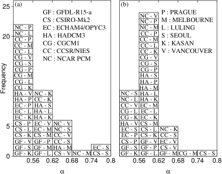
Figure 3: Histogram of the fluctuation exponent ($\alpha$) values obtained for the six sites simulated by the seven AOGCMs (a) scenario (i) and (b) scenario (ii) for the entire records. The entries in each box represent ‘Model – Site’.

For reviewing the scaling performance of the models we concentrate now on the results of DFA3, since DFA3, DFA4 and DFA5 yielded the same scaling exponents for all cases. We find that the fluctuation function in DFA3–5 remained unchanged while FA is changed dramatically when including also future data (see Figure 1). This feature shows some internal consistency of the models, since past and future differ mainly in the amount of trends created by greenhouse gases (as shown by the FA curves), and trends are well eliminated by higher order DFA FN3 . Therefore, we use the entire data for a more accurate estimation of scaling exponents.

Figure 2 shows the results for the fluctuation function obtained from DFA3 for all available real and model data (all seven AOGCMs with scenario (i)) at the six sites considered, for the entire simulation period. To facilitate the evaluation of the models, we have divided $F(s)$ by $s^{\frac{1}{2}}$. A plateau now indicates loss of long term correlations. The straight line in each panel has a slope of 0.15, corresponding to the universal exponent in the original curves. While the real data yield, for long times, parallel lines with a slope of 0.15 for all sites in agreement with the earlier findings, the virtual data display wide performance differences and fail to reproduce the universal features of the benchmark time series. Direct inspection of the figure shows that about half of the model curves are very close to a plateau, yielding uncorrelated behavior above approximately 2 years.

The actual long term exponents $\alpha$ for the greenhouse gas only scenario obtained by the seven models for the six sites are summarized in a histogram in Figure 3a. The histogram shows a pronounced maximum at $\alpha=0.5$. For best performance, all models should have exponents $\alpha$ close to 0.65, corresponding to a peak of height 42 in the window between 0.62 and 0.68. Actually more than half of the exponents are close to 0.5, while only 6 exponents are in the proper window between 0.62 and 0.68.

Figure 3b shows the histogram for scenario (ii), where in addition to the greenhouse gas forcing, also the effects of aerosols are taken into account. For this case, there is a pronounced maximum in the $\alpha$ window between 0.56 and 0.62 (more than half of the exponents are in this window), while only 5 exponents are in the proper range between 0.62 and 0.68. This shows that although the second scenario is also far from reproducing the scaling behavior of the real data, its overall performance is better than the performance of the first scenario.

To summarize, we have presented evidence that AOGCMs fail to reproduce the universal scaling behavior observed in the real temperature records. Moreover, the models display wide differences in scaling for different sites. When comparing the two scenarios, our results suggest that the second scenario (CO₂ plus aerosols) exhibits better performance regarding the values of the scaling exponents as well as the trends. The effect of aerosols not only decreases the trends but also modifies the fluctuations, to more closely resemble the real data. This confirms in a way independent of the evaluations made so far WGI that the incorporation of aerosols is necessary to approach reality.

It is possible that the lack of long-term persistence is due to the fact that certain forcings like volcanic eruptions or solar fluctuations have not been incorporated in the models. However, we cannot rule out that systematic model deficiencies (such as the use of equivalent CO₂ forcing to account for all other greenhouse gases or inaccurate spatial and temporal distributions of sulphate emissions) prevent the AOGCMs from correctly simulating the natural variability of the atmosphere.

- (1) H. Grassl, Science 288, 1991 (2000).
- (2) K. Hasselmann, Nature 390, 225 (1997).
- (3) A typical climate module within the AOGCM machinery will have a grid spacing of 300–500 km and 10–20 vertical layers as compared to a weather forecasting model with a grid spacing of 100 km or less and 30–40 layers.
- (4) http://ipcc-ddc.cru.uea.ac.uk/dkrz/dkrz_index.html
- (5) Climate Change 2001: The Scientific Basis, Contribution of Working Group I to the Third Assessment Report of the Intergovernmental Panel on Climate Change (IPCC) edited by J.T. Houghton et al. (Cambridge University Press, Cambridge, 2001).
- (6) The models also predict climate warming with a global mean increase during the 21st century, in the range of 1.5–4.5 ∘C for greenhouse gas forcing only and 1.0–3.5∘C for greenhouse gas plus sulphate aerosol forcing, depending upon the model.
- (7) J. R. Petit et al., Nature 399, 429 (1999).
- (8) A. Ganopolski et al., Clim. Dynam. 17, 735 (2001).
- (9) S. V. Buldyrev et al., Phys. Rev. E 51, 5084 (1995); C.-K. Peng et al., Phys. Rev. E 49, 1685 (1994).
- (10) J. W. Kantelhardt et al., Physica A 295, 441 (2001).
- (11) E. Koscielny-Bunde et al., Phys. Rev. Lett. 81, 729 (1998).
- (12) E. Koscielny-Bunde et al., Physica A 231, 393 (1996).
- (13) A. Arneodo et al., Phys. Rev. Lett. 74, 3293 (1995).
- (14) J. D. Pelletier, and D. L. Turcotte, J. Hydrol. 203, 198 (1997).
- (15) P. Talkner, and R. O. Weber, Phys. Rev. E 62, 150 (2000).
- (16) M. F. Shlesinger, B. J. West, and J. Klafter, Phys. Rev. Lett. 58, 1100 (1987).
- (17) H. E. Stanley et al., Phil. Mag. B 77, 1373 (1998).
- (18) Fractals in Science edited by A. Bunde, and S. Havlin (Springer, New York, 1995).
- (19) J. Feder, Fractals, (Plenum Press, New York, 1989).
- (20) The large differences between FA and DFA reemphasize that FA (like Hurst method) can not be used by itself for evaluating the scaling exponent.