Quantum in-plane magnetoresistance in 2D electron systems

Abstract

We review various aspects of magnetoresistance in (quasi-)twodimensional systems subject to an in-plane magnetic field. Concentrating on single-particle effects, three mechanisms leading to magnetoresistance are discussed: the orbital effect of the magnetic field – due to inter-subband mixing – and the sensitivity of this effect to the geometrical symmetry of the system, the interplay between spin-orbit coupling and Zeeman splitting, and the influence of the field on spin scattering at magnetic impurities.

I Introduction

Studies of low-dimensional electron systems subject to an in-plane magnetic field have come to the focus of intense attention recently. In several experiments the influence of an in-plane magnetic field on two- and one-dimensional electrons in semiconductor heterostructures [1, 2] as well as in lateral quantum dot devices [3] has been investigated. The use of the fairly unconventional in-plane field geometry aimed at achieving a stronger magnetic field influence on the 2D electron spin, thus, compensating the dominance of orbital effects in most of the known semiconductor materials. Then, by manipulating the field-induced spin polarization, one may extract information about the ground state properties of interacting electrons. At low temperatures – i.e., in the regime where electron-electron interactions open the possibility of a metal-insulator transition or the ferromagnetic Stoner instability – interaction effects coexist with single-particle interference effects. The aim of this article is to provide a theoretical overview of possible influences of an in-plane magnetic field on single-particle quantum transport phenomena in semiconductor heterostructures, quantum wells, and lateral dots.

Quantum transport phenomena have been the subject of extensive experimental and theoretical investigations during recent decades [4, 5, 6, 7]. There exists a broad variety of electronic systems, where spectacular effects produced by the interference of electron waves have been observed. These include weak localization (WL) [8], leading to the low-temperature magnetoresistance in low-dimensional electron structures, such as two-dimensional electron and hole gases in semiconductor heterostructures and quantum wells, as well as universal conductance fluctuations (UCF) [9, 10, 11, 12] in quantum wires and dots.

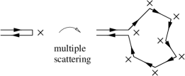
FIG. 1.: Back-scattering from an impurity: Contributions due to multiple scattering events.

Weak localization of electron waves is the result of an enhancement of back-scattering from a scattering center in a disordered environment. This enhancement of back-scattering suppresses electrical conductivity of a quantum conductor, as compared to the value expected on the basis of a classical Drude formula. The Drude result is determined by the mean free path corresponding to a single-impurity scattering cross section whereas multiple scattering events as depicted in Fig. 1 are responsible for the enhanced back-scattering. It is generated by the constructive interference between pairs of electron waves that scatter from the same impurities, i.e., two electron waves arrive together at a particular impurity, scatter from it to follow a random-walk path (in the form of a closed loop) visiting the same set of surrounding impurities – either in clockwise or anti-clockwise direction – and finally scatter into the exactly backward direction. An illustration of electron paths involved in such a non-local scattering process is shown in Fig. 2. Obviously, the observation of such an interference effect requires phase-coherent propagation along the closed-loop part of the geometrical trajectory. Furthermore, the magnitude of the observable contribution to the conductivity is sensitive to the fundamental symmetries of the system, in particular, to the presence or absence of time-reversal (${\cal T}$) symmetry.

The effect of enhanced back-scattering off an impurity inside a disordered metal can be discussed in the same terms as the enhancement of back-scattering of waves from a diffusive medium. The probability $w_{{\bf k},-{\bf k}}$ of a wave to be reflected back from a medium after multiple scattering inside is determined as the modulus of the sum of amplitudes $A_{j}$ corresponding to particular paths $j$,

$$w_{{\bf k},-{\bf k}}=\Bigg{|}\sum_{j}\left[A_{j}^{\circlearrowright}({\bf k},-{\bf k})+A_{j}^{\circlearrowleft}({\bf k},-{\bf k})\right]\Bigg{|}^{2}.$$ (1)

Here, $\circlearrowright$ ($\circlearrowleft$) stands for clockwise (anti-clockwise) propagation along the path.

In an ideally time-reversible system, the two amplitudes related to the electron propagation along the same geometrical loop ‘$j$’ in opposite directions, $A_{j}^{\circlearrowright}({\bf k},-{\bf k})$ and $A_{j}^{\circlearrowleft}({\bf k},-{\bf k})$, are identical. Thus, $A_{j}^{\circlearrowright}A_{j}^{\circlearrowleft\ast}=|A_{j}^{\circlearrowright}|^{2}$, though for each particular loop $A_{j}$ contains a possibly large random semiclassical phase of propagation. The cancellation of phase factors happens because for an electron described by a ${\cal T}$-symmetric Hamiltonian, (a) the phases acquired along the same ‘free’ segment of the path are equal for waves propagating with the wave number ${\bf k}$ and $-{\bf k}$, and (b) the amplitudes of intermediate scattering processes, ${\bf k}_{a}\to{\bf k}_{b}$ for ${\circlearrowright}$ and $-{\bf k}_{b}\to-{\bf k}_{a}$ for ${\circlearrowleft}$ also equal each other at each node of the loop $j$. Therefore, after averaging over different loops which is equivalent to the averaging over disorder, one can identify two phase-insensitive contributions to the back-scattering probability,

$$w_{{\bf k},-{\bf k}} = \sum_{j}\left\langle\big{|}A_{j}^{\circlearrowright}\big{|}^{2}+\big{|}A_{j}^{\circlearrowleft}\big{|}^{2}\right\rangle+2\mathop{\rm Re}\sum_{j}\left\langle A_{j}^{\circlearrowright}A_{j}^{\circlearrowleft\ast}\right\rangle$$ (2)

$$= w^{{\rm class}}+\delta w^{{\rm WL}},$$ (3)

where $w^{{\rm class}}$ is the back-scattering probability of a classical particle whereas $\delta w^{{\rm WL}}$ is an additional quantum contribution due to constructive interference between time-reversed paths. This second term in Eq. (3) increases the return probability, i.e., the probability for an electron to revisit the same scatterer again – which explains the name ‘weak localization’ given to this effect.

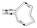
FIG. 2.: Enhanced back-scattering caused by the interference of electrons traveling along the same geometrical path in opposite directions.

The length of closed paths contributing to the interference between back-scattered waves is limited by the phase coherence time $\tau_{\phi}$, yielding a maximal length ${\cal L}_{\rm max}=v_{\rm F}\tau_{\phi}$. In practice, this time scale is determined either by phase relaxation within the system or the electron escape from a fully phase-coherent conductor to bulk reservoirs. Estimates for the weak localization corrections to the conductance read

$$\delta g^{{\rm WL}}\sim-\,\frac{e^{2}}{h}\times\left\{\begin{array}[]{cl}\ln{\displaystyle\frac{\tau_{\phi}}{\tau}}&\qquad{\rm 2D,}\\ {\displaystyle\frac{1}{\sqrt{D\tau_{\phi}}}}&\qquad{\rm Q1D\enspace wire,}\\ 1&\qquad{\rm 0D\enspace dot.}\end{array}\right.$$ (7)

For the case of a dot, by $g$ we understand its full conductance. Furthermore, $\tau$ is the elastic mean free path, and $D=v_{\rm F}^{2}\tau/d$ ($v_{\rm F}$ Fermi velocity, $d$ dimensionality of the system) is the diffusion constant.

The violation of ${\cal T}$-invariance lifts the equivalence between the amplitudes $A_{j}^{\circlearrowright}$ and $A_{j}^{\circlearrowleft}$ and, thus, suppresses contributions to the enhanced back-scattering probability from longer paths. An obvious reason for $t\to-t$ symmetry breaking is an external magnetic field: thus, provided the orbital electron motion is coupled to the field, it affects the interference effects in the phase-coherent electron transport. For two-dimensional electrons in a heterostructure subject to a magnetic field perpendicular to the 2D plane, the difference between the amplitudes $A_{j}^{\circlearrowright}$ and $A_{j}^{\circlearrowleft}$ arises due to the Aharonov-Bohm phases accumulated along the path. For clockwise and anti-clockwise propagation around the oriented area $S_{j}$, the Aharonov-Bohm phases, $\delta\varphi_{\rm AB}=B_{z}S_{j}/\phi_{0}$ ($\phi_{0}$ flux quantum), have opposite signs. As for random-walk trajectories the encircled area $S_{j}$ is random, contributions from paths encircling a magnetic flux larger than typically the flux quantum ($\left|B_{z}S_{j}\right|\gtrsim\phi_{0}$) cancel out after disorder averaging: $\langle A_{j}^{\circlearrowright}A_{j}^{\circlearrowleft\ast}\rangle=\langle\,|A_{j}^{\circlearrowright}|^{2}\times\exp[2i\delta\varphi^{\circlearrowright}_{\rm AB}]\,\rangle\to 0$.

When the orientation of the applied magnetic field lies within the plane of the heterostructure where an effectively two-dimensional electron moves (i.e., $B_{z}=0$), an analysis of its influence on the weak localization properties requires taking into account more subtle arguments than a straightforward consideration of the Aharonov-Bohm effect. In fact, a strictly 2D system is insensitive to the orbital ${\cal T}$-breaking effect of an in-plane magnetic field. A possibility to couple a 2D orbital motion of the electrons to the in-plane magnetic field and, therefore, to break the time-reversal symmetry in a 2D system appears only after taking into account [13, 14, 15, 16, 17] the finite extent of electronic wave functions in the confinement direction of a quantum well as well as subband mixing by the magnetic field [18, 19, 20, 21] and possibly by disorder.

In Chapter III, we discuss this purely orbital effect of an in-plane magnetic field on quantum interference in 2D semiconductor structures. As for the confinement of the transverse motion, we also describe the crossover from the quantum limit (where the width of the system is of order of the Fermi wavelength) to the semiclassical regime corresponding to thin films of disordered and pure metals  [22, 23, 24, 13, 25, 15, 17]. The calculation aims at identifying the time scale $\tau_{B}$ after which the time-reversal symmetry breaking sufficiently affects the phase of an electron to destroy constructive interference. Correspondingly, only paths with lengths shorter than ${\cal L}(B)\sim v_{{\rm F}}\tau_{B}$ contribute to weak localization. Thus, $\tau_{B}$ is the time scale that determines the estimates for the weak localization correction to the conductivity, i.e., it replaces the phase coherence time in Eq. (7). Therefore the conductance is field-dependent, and the so-called magnetoconductance $\Delta g_{B}=\delta g^{{\rm WL}}(B)-\delta g^{{\rm WL}}(0)$ obtains as

$$\Delta g_{B}\sim\,\frac{e^{2}}{h}\times\left\{\begin{array}[]{cl}\ln{\displaystyle\frac{\tau_{\phi}}{\tau_{B}}}&\qquad{\rm 2D,}\\ {\displaystyle\frac{1}{\sqrt{D\tau_{\phi}}}}-{\displaystyle\frac{1}{\sqrt{D\tau_{B}}}}&\qquad{\rm Q1D\enspace wire.}\end{array}\right.$$ (10)

More details about the multi-subband case can be found in chapter VI.

Another possibility for the in-plane magnetic field to affect the interference of 2D electron waves arises due to the coupling between orbital motion and electron spin, which is a pronounced feature of the electronic band structure of most III-V semiconductors with the zinc-blend type crystalline lattice and a unit cell without inversion symmetry. In a heterostructure or quantum well, spin-orbit coupling for a spin-$\frac{1}{2}$ carrier is linear, both in the planar momentum ${\bf k}$ and the spin operator $\underline{\sigma}$. For a given initial spin-polarized state, it produces an electron spin precession, where the precession axis as well as the precession frequency depend on the direction and value of the Fermi momentum of the propagating electron. For a diffusing electron, such a precession randomly changes direction, thus, providing spin relaxation for an initially spin-polarized particle – the mechanism known as Dyakonov-Perel relaxation [26]. However, spin-orbit coupling alone does not violate time-reversal symmetry, though it does modify the above-described interference effects. In particular, strong spin-orbit coupling changes the constructive interference between electrons encircling the same closed geometrical path in opposite directions into destructive interference [27, 28, 29]. To trace the origin of this change, let us consider the extreme limit of dominant spin-orbit coupling, where an electron always remain in the same chiral state along its orbital motion (for instance, $\xi=\frac{{\bf k}}{|{\bf k}|}\cdot\underline{\sigma}=+1$). Thus, an electron approaching the scattering medium in the initial state $|{\bf k},\xi\rangle$ (which can be viewed as $|{\bf k},\rightarrow\rangle$) ends up in the final backward moving state $|\!-\!{\bf k},\xi\rangle$ (which can be viewed as $|\!-\!{\bf k},\leftarrow\rangle$). This implies a rotation of its spin within the $x-y$ plane by the angle $|\theta_{j}|=(2n+1)\pi$ (where $n\in{\mathbb{N}}$) while moving along a diffusive path connecting these two states. For two spin-$\frac{1}{2}$ electrons encircling the same closed loop in opposite directions, $\theta_{j}^{\circlearrowleft}=-\theta_{j}^{\circlearrowright}=(2n+1)\pi$. As a result, their interference produces a negative contribution to the back-scattering,

$$A_{j}^{\circlearrowright}A_{j}^{\circlearrowleft\ast}=\big{|}A_{j}^{\circlearrowright}\big{|}^{2}\exp\left[\frac{i}{2}(\theta_{j}^{\circlearrowright}-\theta_{j}^{\circlearrowleft})\right]=-\big{|}A_{j}^{\circlearrowright}\big{|}^{2},$$ (11)

which increases the quantum conductance as compared to its classical Drude value – the effect known as weak anti-localization.

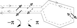
FIG. 3.: Suppressed back-scattering in the presence of strong spin-orbit coupling.

Now, the application of an in-plane magnetic field causes a Zeeman splitting of spin-$\uparrow$ and spin-$\downarrow$ electron states which – in combination with spin-orbit coupling – affects the interference of back-scattered waves. Chapter IV is devoted to the description of the interplay between Zeeman splitting and spin-orbit coupling in determining quantum transport characteristics (in particular, of lateral dots).

Interference between different paths not only affects the mean value of the conductance (i.e., $\langle g\rangle=g_{\rm class}+\delta g^{\rm WL}$) but also characteristic deviations from that mean value, $g=\langle g\rangle+\delta g$. Universal conductance fluctuations (UCF) represent another interference phenomenon observed in mesoscopic conductors and quantum dots at low temperatures. To discuss this effect, let us consider the transmission probability through a disordered piece of metal. For a diffusing electron wave, there are many scenarios leading it from the same initial state $|{\bf k}\rangle_{{\rm left}}$ on the left to the same final state $|{\bf k}^{\prime}\rangle_{{\rm right}}$ on the right, thus, creating the possibility for interference. Depending on the individual distribution of scatterers in the sample, different paths $j$ have different weights – and, thus, the waves following them acquire different phases – which makes the transmission probability,

$$P_{{\bf k},{\bf k}^{\prime}}=\Bigg{|}\sum_{j}A_{j}({\bf k},{\bf k}^{\prime})\Bigg{|}^{2}=\sum_{j}\big{|}A_{j}\big{|}^{2}+\sum_{ji}A_{j}A_{i}^{\ast}\;,$$ (12)

sample-specific as well as dependent on specific interference conditions, namely the energy (wavelength) of the incident electron or the presence of an external magnetic field. In measurements, this manifests itself in a random but reproducible dependence of the sample conductance on the Fermi energy $E_{{\rm F}}$ and the applied field $B_{z}$. Furthermore, gate voltages (varying the shape of a semiconductor dot) represent an additional control parameter.

In a phase-coherent system, the variance of conductance fluctuations has a value,

$$\langle\delta g^{2}\rangle=c_{{\rm geom}}\,\alpha\times\,\left(\frac{e^{2}}{h}\right)^{2},$$ (13)

which is universal [9, 10, 11, 30, 31] up to a geometry-dependent numerical factor $c_{{\rm geom}}\sim 1$. Furthermore, $\alpha$ reflects the fundamental symmetries of the system, expressed by three coefficients,

$$\alpha=\frac{s}{\beta\Sigma}.$$ (14)

The symmetry plays such an important role here as it determines the number of independently fluctuating components of the generically random amplitudes $A_{j}$ related to each particular geometrical path. The higher the symmetry, the more correlations are implicit between real and imaginary parts as well as spin components of $A_{j}$. In particular, $s=1$ or $2$ depending on whether Kramers’ degeneracy is lifted or not. When the orbital electron motion is independent of the electron spin state, i.e., when the system possesses spin-rotation invariance, the ${\cal T}$-symmetric system is described by $\beta=1$ whereas $\beta=2$ if time-reversal symmetry is broken. The value $\beta=4$ (with $s=1$) represents the case of efficient spin-relaxation due to spin-orbit scattering. Finally, an additional symmetry class number $\Sigma$ [31] characterizes whether a violation of time-reversal symmetry in the spin-sector affects ($\Sigma=2$ – or not, $\Sigma=1$) the interference in the electron orbital motion via spin-orbit coupling. The crossover between the latter two symmetry classes may be achieved by varying the Zeeman splitting. Its features will be described in Chapter IV, together with weak localization effects.

As phase coherence is crucial for the occurrence of interference effects, the influence of symmetry breaking on conductance measurements is not observable when the corresponding time scale is larger than the decoherence time, $\tau_{B}>\tau_{\varphi}$. As for finite systems, when decoherence of electrons in a dot or a short wire happens faster than the escape into bulk reservoirs, $\tau_{\varphi}<\tau_{{\rm esc}}$, both the enhanced back-scattering effect and UCFs get suppressed [32, 33] as compared to the conductance quantum, $e^{2}/h$. In these situations, no influence of an in-plane magnetic field on quantum transport characteristics of the system would be expected – unless the field affects the decoherence time.

This is the case when the latter is caused by spin-flip scattering at paramagnetic impurities [34]. In all foreseeable regimes [34, 35], degenerate paramagnetic impurities destroy weak localization via spin-flip scattering, the relevant time scale being the spin-flip scattering time $\tau_{\rm s}$. Furthermore, they suppress conductance fluctuations [36, 37, 38, 39, 40] as the flipping of impurity spins effectively changes the realization of disorder in the sample and, thus, leads to a self-averaging of the conductance. However, a Zeeman splitting of the magnetic impurity levels by a magnetic field causes an energy threshold for electron spin-flip processes which slows down the electron spin relaxation. At a high field, the electron spin relaxation is possible only due to very few thermally activated impurity spins, so its rate is reduced by the exponential factor, $\tau_{s}^{-1}(B)\propto\tau_{s}^{-1}\times\exp[-g^{{\rm(imp)}}\mu_{\rm B}B/T]$, where $\mu_{\rm B}$ is the Bohr magneton and $g^{{\rm(imp)}}$ the $g$-factor of the impurities. Thus, a sufficiently strong magnetic field restores UCFs [36, 38, 39, 40] as well as weak localization (if the orbital effect of the magnetic field is excluded). The in-plane magnetoresistance of magnetically contaminated 2D semiconductors and other features related to the dynamics of paramagnetic impurities are discussed in Chapter V.

For all practical purposes, the study of symmetry breaking rates, determining the parallel field effect on the weak localization corrections to the conductivity of a 2D electron gas or a semiconductor wire, can be completed using the diagrammatic perturbation theory for disordered systems. Although one can find more details about this technique in several textbooks and review articles (see, e.g., [41]), for the sake of completeness, we describe its necessary elements in Chapter II. As an alternative, field theoretic methods may be used. In chapter VI, we illustrate the supersymmetric non-linear sigma-model in application to one of the problems listed above, i.e., the orbital effect of an in-plane magnetic field (via subband mixing) on the transport properties of 2D electrons.

II The diagrammatic technique: diffusons and Cooperons

Diagrammatics is a perturbative method which allows one to a) classify different contributions to the perturbation series and b) sum up the relevant terms. To be specific, here – for simplicity – we choose the random disorder potential $V$ to be drawn from a Gaussian white noise distribution:

$$\langle V({\bf r})\rangle=0,\qquad\langle V({\bf r})V({\bf r}^{\prime})\rangle=\frac{1}{2\pi\nu\tau}\delta({\bf r}-{\bf r}^{\prime}),$$ (15)

where $\nu$ is the density of states (DoS) at the Fermi level and $\tau$ is the mean free scattering time. Note that throughout this review we will use units where $\hbar=c=e=1$.

The starting point of the perturbative approach is the representation of the Green function as a series in powers of $V$, i.e., $G=G_{0}+G_{0}\sum_{n}(VG_{0})^{n}$. Under averaging, diagrams with single impurity lines vanish (due to $\langle V\rangle=0$). Thus, the diagrammatic expansion involves only diagrams with paired impurity lines. The average Green function is then given by a Dyson equation, depicted schematically in Fig. 4:

$$\langle G\rangle=G_{0}+G_{0}\sum_{n=1}^{\infty}(\Sigma G_{0})^{n}=G_{0}+G_{0}\Sigma\langle G\rangle\quad\Longleftrightarrow\quad\langle G\rangle=\frac{G_{0}}{1-\Sigma G_{0}},$$ (16)

where the self-energy $\Sigma$ contains all irreducible diagrams, i.e., diagrams that cannot be split into two by cutting one $G_{0}$-line.

FIG. 4.: Diagrammatic representation of the Dyson equation.

The dominant contribution to the self-energy reads

$$\Sigma_{0}^{\pm}({\bf p})=\left\langle\int\!d{\bf q}\;V({\bf q})G_{0}^{\pm}({\bf p}-{\bf q};\epsilon)V(-{\bf q})\right\rangle,$$ (17)

where the shorthand notation $d{\bf q}=d^{d}q/(2\pi)^{d}$ has been introduced. Since the potential is $\delta$-correlated in real space, its Fourier transform does not depend on momentum. Hence, $\Sigma_{0}^{\pm}=\int\!d{\bf p}\,G_{0}^{\pm}({\bf p};\epsilon)/(2\pi\nu\tau)$.

The real part of $\Sigma$, leading to a shift in energy, can be absorbed in the ground state energy. Using that the unperturbed Green function reads $G_{0}^{\pm}({\bf p};\epsilon)=(\epsilon\pm i0+\xi_{{\bf p}})^{-1}$, where $\xi_{{\bf p}}=\epsilon_{\rm F}-p^{2}/(2m)$, and the definition of the density of states, $\nu(\epsilon)=L^{-d}\sum_{\bf p}\delta(\epsilon+\xi_{{\bf p}})$, the imaginary part of $\Sigma$ obtains

$$\Im\,\Sigma_{0}^{\pm}=\mp\frac{1}{2\nu\tau}\int\!d{\bf p}\,\delta(\epsilon+\xi_{{\bf p}})=\mp\frac{1}{2\tau}.$$ (18)

The associated length scale $\ell$ is the decay length of the average Green function as we will see shortly. In the case of weak disorder, $\tau^{-1}\ll\epsilon_{\rm F}$, all other contributions are small in $1/(k_{\rm F}\ell)$, and Eq. (18) determines the self-energy $\Sigma$ in the self-consistent Born approximation (SCBA).

Inserting the above result into the Dyson equation yields

$$\langle G^{\pm}\rangle({\bf p};\epsilon) = \frac{1}{\epsilon+\xi_{{\bf p}}\pm\frac{i}{2\tau}}.$$ (19)

In real space representation, this leads to a decay of the average Green function on the scale of the mean free path,

$$\langle G\rangle({\bf r},{\bf r}^{\prime})=G_{0}({\bf r},{\bf r}^{\prime})\,e^{-\frac{|{\bf r}-{\bf r}^{\prime}|}{2\ell}}.$$ (20)

Having found the average Green function, the next step is to calculate correlation functions of the form

$$F({\bf p}_{1},{\bf p}_{1}^{\prime},{\bf p}_{2},{\bf p}_{2}^{\prime};\omega)=\langle G^{-}({\bf p}_{1},{\bf p}_{1}^{\prime};\epsilon)G^{+}({\bf p}_{2},{\bf p}_{2}^{\prime};\epsilon+\omega)\rangle.$$ (21)

Again – as for the averaged Green function – the diagrammatic perturbation series involves summing up diagrams with paired impurity lines. The dominant contributions are series of ladder diagrams and maximally crossed diagrams, see Fig. 5. With the notation $\langle AB\rangle_{c}=\langle AB\rangle-\langle A\rangle\langle B\rangle$, i.e., subtracting the disconnected part of the correlator, the contribution of connected diagrams can be written as

$$\langle G^{-}({\bf p}_{1},{\bf p}_{1}^{\prime};\epsilon)G^{+}({\bf p}_{2},{\bf p}_{2}^{\prime};\epsilon+\omega)\rangle_{c}$$ (22)

$$= \langle G^{-}\rangle({\bf p}_{1},\epsilon)\,\langle G^{-}\rangle({\bf p}_{1}^{\prime},\epsilon)\,\langle G^{+}\rangle({\bf p}_{2},\epsilon+\omega)\,\langle G^{+}\rangle({\bf p}_{2}^{\prime},\epsilon+\omega)\rangle\Gamma({\bf p}_{1},{\bf p}_{2},{\bf p}_{1}^{\prime},{\bf p}_{2}^{\prime};\omega)\,\delta({\bf p}_{1}-{\bf p}_{2}-{\bf p}_{1}^{\prime}+{\bf p}_{2}^{\prime}),$$ (23)

thus defining the reducible vertex function $\Gamma({\bf p}_{1},{\bf p}_{2},{\bf p}_{1}^{\prime},{\bf p}_{2}^{\prime};\omega)$.

FIG. 5.: Ladder and maximally crossed diagrams.

Consider first the sum of ladder diagrams depicted in the upper part of Fig. 5. Due to momentum conservation at each vertex, the momentum difference ${\bf q}\equiv{\bf p}_{1}\!-\!{\bf p}_{2}(={\bf p}_{1}^{\prime}\!-\!{\bf p}_{2}^{\prime})$ is constant, and $\Gamma$ depends on this difference only. Then $\Gamma({\bf q},\omega)$ is given by a Bethe-Salpeter equation, the two-particle analogue of the Dyson equation:

$$\Gamma({\bf q},\omega)=\gamma+\gamma\Big{[}\underbrace{\int d{\bf p}^{\prime\prime}\,\langle G^{-}\rangle({\bf p}^{\prime\prime}+{\bf q},\epsilon+\omega)\langle G^{+}\rangle({\bf p}^{\prime\prime},\epsilon+\omega)}_{\textstyle\equiv\Pi({\bf q},\omega)}\Big{]}\Gamma({\bf q},\omega),$$ (24)

where $\gamma=1/(2\pi\nu\tau)$. Anticipating the result that $\Gamma$ diverges for ${\bf q},\omega\rightarrow 0$, we can approximate the irreducible vertex function $\Pi$ for small $|{\bf q}|,\omega$:

$$\Pi({\bf q},\omega)\simeq 2\pi\nu\tau(1+i\omega\tau-D{\bf q}^{2}\tau),$$ (25)

where $D=v_{\rm F}^{2}\tau/d$ is the diffusion constant ($d$ dimensionality of the system). Thus, the sum of ladder diagrams finally yields

$$\Gamma({\bf q},\omega)=\frac{\gamma}{1-\gamma\,\Pi({\bf q},\omega)}=\frac{1}{2\pi\nu\tau^{2}}\frac{1}{D{\bf q}^{2}-i\omega}\equiv{\cal D}({\bf q},\omega).$$ (26)

This is a diffusion pole or so-called diffuson. It can easily be seen that the diffuson is not affected by a weak magnetic field: Minimal coupling implies that the magnetic field shifts all momenta by the corresponding vector potential, ${\bf p}\to{\bf p}-{\bf A}$; however, $({\bf p}_{1}-{\bf A})-({\bf p}_{2}-{\bf A})={\bf p}_{1}-{\bf p}_{2}={\bf q}$.

A maximally crossed diagram [42] (for a detailed discussion see e.g. [43]) can be converted to a ladder by reversing one $G$-line. Since now all the arrows point in the same direction, momentum conservation at the vertices requires the momentum sum ${\bf Q}={\bf p}_{1}\!+\!{\bf p}_{2}^{\prime}$ to be constant. Apart from that, the structure of all equations is the same as for the ladder diagrams. Thus,

$$\Gamma({\bf Q},\omega)=\frac{1}{2\pi\nu\tau^{2}}\frac{1}{D{\bf Q}^{2}-i\omega}\equiv{\cal C}({\bf Q},\omega).$$ (27)

This is called a Cooperon – in analogy to superconductivity, as it corresponds to a correlator in the particle-particle channel (as opposed to the particle-hole channel for the diffuson). Now the presence of a magnetic field requires replacing ${\bf Q}\to{\bf Q}-2{\bf A}$ which leads to a decaying of the Cooperon.

Taking into account the spin of the electrons, diffusons and Cooperons split into singlet and triplet modes. This will become important when considering spin-orbit coupling or spin scattering. Details will be given in the corresponding chapters IV and V.

In coordinate representation, the expression obtained in Eq. (27) has the form of a diffusion equation,

$$[D(\nabla+i2{\bf A})^{2}-i\omega]{\cal C}=\delta({\bf x}-{\bf x^{\prime}}).$$ (28)

(A similar equation holds for the diffuson, Eq. (26).) In a finite size geometry, this equation should be complemented by boundary conditions. For an ‘open’ surface, as, e.g., the interface with a bulk reservoir, the boundary condition reads

$${\cal C}=0.$$ (29)

For an insulating surface, for example, the edge of a metallic dot, the corresponding boundary condition expresses the lack of a phase-coherent current density across the sample surface,

$${\bf n}_{\parallel}\cdot(\nabla+i2{\bf A}){\cal C}=0,$$ (30)

where ${\bf n}_{\parallel}$ is a unit vector normal to the sample surface. In the case of zero magnetic field, this boundary condition indicates that the lowest Cooperon and diffuson modes correspond to the constant ($Q=0$) solution and are gapless. This choice of the lowest mode, being constant in space, is called the zero-dimensional (0D) approximation. In the presence of a magnetic field, one has to give the analysis of the lowest modes in closed systems more attention, applying a gauge transformation to the gauge where ${\bf n}_{\parallel}\cdot{\bf A}=0$, and only then making the 0D approximation. Subsequently, the discrete spectrum of relaxational modes describing the Cooperon and diffuson can be found using the standard Hamiltonian perturbation theory methods. This is a useful trick which enables us find the Cooperon and diffuson functions and, in particular, their lowest eigenmodes in finite size geometries.

III In-plane magnetoresistance effect due to intersubband mixing

As pointed out in the introduction, the influence of an in-plane magnetic field on the quantum transport characteristics of a 2D or quasi-2D system can be divided into orbital and spin-related effects. In this section, we consider the orbital effect – treating electrons as spinless.

There are two features that make the issue of the influence of an in-plane magnetic field on quantum interference effects in inversion layers and thin metallic films non-trivial. The first issue is related to the fact that a finite spatial extent of electron wave functions along the confinement direction, i.e., the $z$-direction perpendicular to the 2D plane, is needed in order that the electron can accumulate an additional magnetic field-induced phase if the field is exactly parallel to the 2D plane. Furthermore, the possible accumulation of such an Aharonov-Bohm phase is sensitive to the inversion symmetry properties of the system. In particular, for a quantum well with a potential profile that is symmetric with respect to the transformation ${\cal P}_{z}:z\rightarrow-z$, an in-plane magnetic field cannot induce any dephazing, and the field-dependent rate $\tau_{B}^{-1}$ is equal to zero. This property reflects the Berry-Robnik symmetry effect [44]: Consider a system described by a Hamiltonian ${\hat{\cal H}}$ that at $B=0$ is invariant under a discrete symmetry transformation, such as ${\cal P}_{z}$, and at finite fields remains invariant under the combined time and $z$-coordinate inversion transformation, ${\cal P}_{z}{\cal T}$, i.e., ${\cal P}_{z}{\cal T}{\hat{\cal H}}(B)={\hat{\cal H}}(B)$. Then there always exist pairs of paths having exactly the same value of the semiclassical action which, therefore, interfere constructively even in the presence of a magnetic field. As a result, the suppression of weak localization by an in-plane magnetic field is possible only if either the scattering potential in the quantum well is $z$-dependent [13] (since a generic $z$-dependence does not respect ${\cal P}_{z}$-symmetry), or if the form of the confinement potential in $z$-direction has no inversion symmetry [15, 16, 17] (as usually is the case for a inversion layer in a heterostructure). In the first subsection, we provide a quantitative analysis of this effect. In the second subsection, this analysis is extended to multi-subband systems [15, 16], and the results are compared to the magnetoresistance in thin films with diffusive transverse motion.

The second non-trivial issue concerns the so-called geometrical flux cancellation characteristic for ballistic metallic films (wires), where electrons scatter only from surface (edge) defects at two parallel surfaces. In such a ‘quasi-ballistic’ film, the finite resistance is provided by the diffusive scattering of carriers from the surface. Quantum corrections to the conductivity are related to the interference between waves propagating along paths consisting of a sequence of ballistic flights between the film edges. Among those paths, the trajectories containing ballistic segments that are almost parallel to the film surface and, therefore, much longer than the film width $d$ play an important role. These so-called Lévy flights (in the terminology of anomalous diffusion theory [45]) produce a logarithmically large contribution to the sample conductance [46]. The oriented area encircled by a closed loop made of quasi-ballistic paths is exactly equal to zero [23], thus suppressing the magnetic field effect on the interference of electron waves propagating along them. An electron can accumulate a magnetic flux only due to a curving of its trajectory by the magnetic field itself. This makes the role of Lévy flights important for the interference-related magnetoresistance of ballistic films and wires: curving of the longest ballistic flights – which is a purely classical effect – switches their scattering at the surface roughness from one film surface (or wire edge) to the other [25]. This peculiar situation and the resulting unexpected influence of a magnetic field on the localization properties in quasi-ballistic wires are discussed at the end of this section.

A Phase-breaking by an in-plane magnetic field in 2D inversion layers

The influence of an in-plane magnetic field on the orbital motion of carriers in a heterostructure or quantum well is a result of the finite width $d$ of any 2D layer. This effect has been discussed previously in various contexts [18, 19, 20, 21]. The Lorentz force on the electrons generated by the in-plane field ${\bf B}_{\|}$ mixes up the electron motion along and across the confinement direction, thus resulting in a modification of the 2D dispersion, $E(p)\rightarrow E({\bf B}_{\|},{\bf p})$. In particular, a) the 2D electron mass increases in the direction perpendicular to ${\bf B}_{\|}$. Furthermore, in heterostructures with a confining potential that does not possess inversion symmetry, b) the in-plane field also lifts the ${\bf p}\to-{\bf p}$ symmetry in the dispersion law [18, 19]:

$$E({\bf B}_{\|},{\bf p})-E({\bf B}_{\|},-{\bf p})\propto\left({\bf p}\cdot[{\bf B}_{\|}\times{\bf e}_{z}]\right)^{3}\neq 0,$$

where ${\bf e}_{z}$ is a unit vector perpendicular to the plane. This leads to a field-dependent suppression of the WL signal as will be discussed below. By contrast, for the $z$-inversion symmetric problem, due to the Berry-Robnik phenomenon [44], the Cooperon mode remains massless, and there is no magnetoresistance.

In the presence of an in-plane magnetic field, the effective 2D Hamiltonian for electrons in a heterostructure with the confining potential profile $W(z)$ can be obtained from the 3D Hamiltonian,

$${\hat{\cal H}}_{3D}=\frac{(-i\nabla-{\bf A})^{2}}{2m}-\frac{\partial_{z}^{2}}{2m}+W(z)+u({\bf r},z),$$ (31)

using a plane wave representation, $\Psi_{{\bf p}}=e^{i{\bf pr}}\phi_{0}^{({\bf p})}(z)$ for the electrons in the lowest subband. Here, $\phi_{k}^{({\bf p})}(z)$ are the eigenfunctions of the $z$-dependent part of the Hamiltonian. In particular, at $B_{\|}=0$, the in-plane and perpendicular motion are separable, and the corresponding eigenfunctions are given by $|k\rangle\equiv\phi_{k}^{({0})}$. Due to the mixing between subbands $|0\rangle$ and $|k\!>\!0\rangle$ by an in-plane magnetic field, the eigenfunction $\phi_{0}^{({\bf p})}(z)$ in the presence of the field depend on the in-plane momentum ${\bf p}$. In order to find $\phi_{0}^{({\bf p})}(z)$ and the corresponding energy $E({\bf B}_{\|},{\bf p})$ for each plane wave state a perturbation theory analysis – as described in the following – or a numerical self-consistent-field technique may be used.

Furthermore, in Eq. (31), the vector potential reads ${\bf A}=(z-z_{0}){\bf B}_{\|}\times{\bf e}_{z}$, where $z_{0}=\langle 0|z|0\rangle$ is the center of mass position of the electron wave function in the lowest subband (at $B_{\|}=0$), and the potential $u({\bf r},z)$ is a combination of the Coulomb potential of impurities and the lateral potential forming the quantum dot.

For weak to intermediate magnetic fields ${\bf B}_{\|}$, the effective 2D Hamiltonian takes the form

$${\hat{\cal H}}_{2D}=\frac{{\bf p}^{2}}{2m}-p_{\bot}^{2}\gamma(B_{\|})+p_{\bot}^{3}\beta(B_{\|})+u({\bf r}).$$ (32)

Here, ${\bf p}=-i\nabla-{\bf a}({\bf r})$ is a purely 2D momentum operator and $p_{\bot}={\bf p}\cdot[\frac{{\bf B}_{\|}}{B_{\|}}\times{\bf e}_{z}]$ its component perpendicular to ${\bf B}_{\|}$.

Thus, the application of an in-plane magnetic fields results in a) an effective vector potential ${\bf a}({\bf r})$, and b) two additional terms in the free electron dispersion due to $p_{\bot}$-dependent inter-subband mixing. The first term, $\delta\hat{\cal H}^{(2)}=-p_{\bot}^{2}\gamma$, lifts the rotational symmetry by causing an anisotropic mass enhancement [18, 19]. It increases the 2D density of states and, for a 2D gas with fixed sheet density, it reduces the Fermi energy calculated from the bottom of the 2D conduction band, i.e., $E_{{\rm F}}(B_{\|})=E_{{\rm F}}^{0}-{\gamma(B_{\|})}p_{{\rm F}}^{2}/2$. The second term, $\delta\hat{\cal H}^{(3)}=p_{\bot}^{3}\beta$, is related to the time-reversal symmetry breaking by $B_{\|}$. A perturbative analysis of the problem results in the field dependences $\gamma\sim B_{\|}^{2}$ and $\beta\sim B_{\|}^{3}$. Indeed, an expansion of the plane-wave energy up to the third order in $p_{\bot}$ yields

$$\gamma(B_{\|}) \approx \frac{B_{\|}^{2}}{m^{2}}\sum_{k\geq 1}\frac{\langle k|z|0\rangle^{2}}{\epsilon_{k}-\epsilon_{0}}\sim\frac{1}{m}\left(\frac{d}{\lambda_{B}}\right)^{4},$$

$$\beta(B_{\|}) \approx \frac{B_{\|}^{3}}{m^{3}}\sum_{k,k^{\prime}\geq 1}\frac{\langle 0|z|k\rangle\langle k|z|k^{\prime}\rangle\langle k^{\prime}|z|0\rangle}{(\epsilon_{k}-\epsilon_{0})(\epsilon_{k^{\prime}}-\epsilon_{0})}\sim\frac{d}{m}\left(\frac{d}{\lambda_{B}}\right)^{6},$$

where $\epsilon_{k}$ are the subband energies and $\lambda_{B}={1/\sqrt{B_{\|}}}$ is the magnetic length.

In ${\hat{\cal H}}_{2D}$ given by Eq. (32), the “in-plane” disorder is incorporated in the form of a scattering potential $u({\bf r})\approx$ $\langle 0|u({\bf r},z)|0\rangle$. It can be characterized by the mean free path, $\ell\gg 1/p_{{\rm F}}$ or, equivalently, the momentum relaxation time $\tau$, related to the diffusion coefficient $D=v_{{\rm F}}^{2}\tau/2$. The modification of the electron density of states by $B_{\|}$ only slightly affects the value of the electron mean free path. However, the presence of a parallel field also changes the symmetry of the Born scattering amplitudes between plane waves, $f_{{\bf pp}^{\prime}}=\langle\Psi_{{\bf p}}|u({\bf r},z)|\Psi_{{\bf p}^{\prime}}\rangle$. Due to the momentum-dependent subband mixing, $f_{{\bf pp}^{\prime}}$ acquires an additional contribution, $f_{{\bf pp}^{\prime}}=f_{{\bf pp}^{\prime}}^{(0)}\left\{1+(p_{\bot}+p_{\bot}^{\prime})B_{\|}\zeta\right\}$, where

$\displaystyle\zeta=\frac{1}{m\langle 0|u({\bf p}-{\bf p}^{\prime},z)|0\rangle}\sum_{k\geq 1}\frac{\langle 0|u({\bf p}-{\bf p}^{\prime},z)|k\rangle\langle k|z|0\rangle}{\epsilon_{k}-\epsilon_{0}}.$

This corresponds to the presence of a random gauge field in the effective 2D Hamiltonian [13, 14, 47],

$\displaystyle{\bf a}({\bf r})=2\sum_{k\geq 1}\frac{\langle 0|u({\bf r},z)|k\rangle\langle k|z|0\rangle}{\epsilon_{k}-\epsilon_{0}}[{\bf B}_{\|}\times{\bf e}_{z}],$

which can be interpreted as a result of an effective ‘curving’ of the 2D plane by impurities with a $z$-dependent scattering potential in the system. In the presence of an in-plane magnetic field this curving generates a random effective perpendicular field component, $b_{\bot}=\left[\nabla\times{\bf a}\right]_{z}$. In systems, where scattering is dominated by Coulomb centers separated from the 2D plane by a spacer and, thus, is almost independent of $z$, a smaller effect may be taken into account, namely $\delta{\bf a}\sim[{\bf B}_{\|}\times{\bf e}_{z}]([{\bf B}_{\|}\times{\bf e}_{z}]\cdot\nabla)^{2}u({\bf r})$. However, $\delta{\bf a}$ has a negligible influence on the quantum transport characteristics of 2D electrons as compared to the effect of the field-dependent electron dispersion.

The perturbative calculation of two-particle correlation functions, i.e., diffusons ${\cal D}({\bf x},{\bf x}^{\prime};\omega)$ and Cooperons ${\cal C}({\bf x},{\bf x}^{\prime};\omega)$ [9, 10, 11], requires taking into account all field-dependent terms in the effective 2D Hamiltonian Eq. (32). Admitting for different magnetic fields ${\bf B}_{\|1}$ and ${\bf B}_{\|2}$, the result for the diffuson has the form

$$\left[-D\nabla^{2}-i\tilde{\omega}+\tau_{{\rm d}}^{-1}\right]{\cal D}=\delta({\bf x}-{\bf x}^{\prime}),$$ (33)

where $\tilde{\omega}=\omega+\delta$ with $\delta=p_{{\rm F}}^{2}[\gamma(B_{\|1})-\gamma(B_{\|2})]/2$. The field-dependent rate $\tau_{{\rm d}}^{-1}(B_{\|1},B_{\|2})$ reads

$$\tau_{{\rm d}}^{-1}=\frac{\tau p_{{\rm F}}^{4}}{8}[\gamma(B_{\|1})-\gamma(B_{\|2})]^{2}+\frac{\zeta^{2}}{2\tau}p_{{\rm F}}^{2}[B_{\|1}-B_{\|2}]^{2}$$ (34)

which vanishes for $B_{\|1}=B_{\|2}$.

The first term in Eq. (34) comes from a deformation of the Fermi circle by the magnetic field $B_{\|}$. The second term takes into account the field effect on the scattering of plane waves. Furthermore, Eq. (33) contains the difference between the electron kinetic energies in two measurements of conductance, $\tilde{\omega}=E_{{\rm F}}(B_{\|1})-E_{{\rm F}}(B_{\|2})$, each of them shifted by the magnetic field with respect to the Fermi energy $E_{{\rm F}}^{0}$ at $B_{\|}=0$ of the electron gas with the same sheet density. The latter fact is important, since, for lateral dots where the electron density is fixed, one should substitute $\tilde{\omega}=0$.

The Cooperon equation can be represented in the form

$$\left[D(-i\nabla-{\bf A}_{0})^{2}-i\tilde{\omega}+\tau_{{\rm d}}^{-1}+\tau_{\rm c}^{-1}\right]{\cal C}=\delta({\bf x}-{\bf x}^{\prime}).$$ (35)

It contains an additional decay rate $\tau_{{\rm c}}^{-1}(B_{\|1},B_{\|2})$ given as

$$\tau_{{\rm c}}^{-1}=\frac{\tau p_{{\rm F}}^{6}}{8}\left[\frac{\beta(B_{\|1})+\beta(B_{\|2})}{2}\right]^{2}+\frac{\zeta^{2}p_{{\rm F}}^{2}}{2\tau}[B_{\|1}+B_{\|2}]^{2}$$ (36)

which accounts for the dephazing of electrons encircling the same chaotic trajectory in opposite directions. Thus, the result of lifting time-reversal symmetry by an in-plane magnetic field can be described by the Cooperon phase-breaking rate

$$\tau_{B\|}^{-1}\equiv\tau_{{\rm c}}^{-1}(B_{\|},B_{\|})=\frac{\tau p_{{\rm F}}^{6}}{8}\beta^{2}(B_{\|})+\frac{2\zeta^{2}p_{{\rm F}}^{2}}{\tau}B_{\|}^{2}\sim aB_{\|}^{6}+bB_{\|}^{2}.$$ (37)

Note the gauge shift in the Cooperon equation (35). The ‘vector potential’ ${\bf A}_{0}=\frac{3}{2}p_{{\rm F}}^{2}m\beta(B_{\|})[\frac{{\bf B}_{\|}}{B_{\|}}\times{\bf e}_{z}]$ results from the following artifact: the cubic term in the effective electron dispersion not only lifts the ${\bf p}\to-{\bf p}$ inversion symmetry of the line $E(B_{\|},{\bf p})=E_{{\rm F}}(B_{\|})$, but also shifts its geometrical center with respect to the bottom of the 2D conduction band. However, since for the conductance only electrons with energy $\epsilon=E_{{\rm F}}$ matter, such a shift can be eliminated by choosing a slightly modified initial gauge. This can be corrected for now by applying a gauge transformation ${\cal C}\to e^{i{\bf qx}}{\cal C}$ directly to the Cooperon. In other words, the phase-coherent transport is only affected by the $B_{\|}$-induced ${\bf p}\rightarrow-{\bf p}$ asymmetric distortion of the Fermi circle into an oval, but not by a shift of its center in the momentum space. That is, only the $B_{\|}$-dependent anisotropy of the electron wavelength along the Fermi line affects the interference pattern of current carriers. Note that both terms in Eq. (37) are non-vanishing only in the absence of $z\to-z$ inversion symmetry.

The phase-breaking rate in Eq. (37) can also be used to describe magnetoresistance and universal conductance fluctuations (UCF) in lateral semiconductor dots. For quantum dots, weak localization corrections and the variance of UCF can be represented as

$\displaystyle g_{{\rm WL}}(B_{\|})\propto\int(d{x})\;W({\bf x})\,{\cal C}({\bf x},{\bf x};0)\equiv\langle g(B_{\|})\rangle-\langle g\rangle_{u},$

where the subscript ‘$u$’ stands for unitary, and

$\displaystyle\langle\delta g(B_{\|1})\delta g(B_{\|2})\rangle\propto\int(d{x})(d{x}^{\prime})\;W({\bf x})W({\bf x}^{\prime})\sum_{{\cal P=D},{\cal C}}|{\cal P}({\bf x},{\bf x}^{\prime};\omega)|^{2},$

where $\omega=E_{{\rm F}}(B_{\|1})-E_{{\rm F}}(B_{\|2})$, and $E_{{\rm F}}(B_{\|})$ is the Fermi energy of the 2D electron gas calculated from the bottom of the conduction band. The dispersionless weight factors $W({\bf x})$ take care of the particle number conservation upon diffusion inside the dot [48] and incorporate the coupling parameters to the leads. In the zero-dimensional limit, both, $g_{{\rm WL}}$ and $\langle\delta g(B_{\|1})\delta g(B_{\|2})\rangle$, are dominated by the lowest (spatially homogeneous) Cooperon (diffuson) relaxation mode $\lambda_{0}$, which is determined by the rate of escape to the reservoirs, $\tau_{{\rm esc}}^{-1}$ $\ll D/L^{2}$ (Thouless energy), and the Cooperon suppression by time-reversal symmetry breaking described by $\tau_{B\|}^{-1}$. The latter expresses the efficient reduction of the fundamental symmetry of the system from orthogonal ($o$) to unitary ($u$). In the absence of spin-orbit effects, the parameters $\tau_{{\rm esc}}^{-1}$ and $\tau_{B\|}^{-1}$ describe the value of WL corrections as well as the variance of UCF, $\langle\delta g^{2}(B_{\|})\rangle$, as compared to their nominal values, $g_{{\rm WL}}(0)\equiv\langle g\rangle_{o}-\langle g\rangle_{u}$ and $\langle\delta g^{2}\rangle_{u}$:

$$g_{{\rm WL}}(B_{\|}) = g_{{\rm WL}}(0)\,\frac{1}{1+\tau_{\rm esc}/\tau_{B}},$$ (38)

$$\langle\delta g^{2}(B_{\|})\rangle = \langle\delta g^{2}\rangle_{u}\left(1+\frac{1}{(1+\tau_{\rm esc}/\tau_{B})^{2}}\right).$$ (39)

Thus, these two parameters can be studied from the UCF fingerprints measured by changing the shape of a dot in multi-gate devices or by varying the Fermi energy in back-gated dots.

FIG. 6.: Calculated dependence of the parameters $\gamma$ and $\beta$ on the sheet density of 2D electrons. The insets show the effect of $B_{\|}$ on the symmetric, $[E({\bf p})+E(-{\bf p})]/2$, and anti-symmetric, $[E({\bf p})-E(-{\bf p})]/2$, parts of the 2D electron dispersion in a broader range of $B_{\|}$, where a perturbative expansion is not applicable.

In ballistic billiards or heterostructures with a $z$-independent impurity scattering potential, the in-plane magnetic field effects are governed by the unusual $B_{\|}^{6}$-dependence of $\tau_{B\|}^{-1}$ [15, 16, 17] that we attribute to the effect of a cubic term in the 2D electron dispersion generated by the field. This should give rise to a relatively sharp crossover between ‘flat’ regions related to regimes with orthogonal and unitary symmetry, respectively. To get an idea about the relevance of this effect for the large-area ($\sim$8$\mu$m²) quantum dots studied by Folk et al [3], quantitative estimates for the parameters $\gamma(B_{\|})$ and $\beta(B_{\|})$ can be obtained by evaluating the electron dispersion within a fully self-consistent numerical method [17]. Using the nominal growth parameters of the Al_.34Ga_.66As/GaAs sample studied in [3], the dependences of $\gamma$ and $\beta$ on the in-plane magnetic field for an electron sheet density of 2$\times$10¹¹ cm^-2 shown in the insets of Fig. 6 a) and b) were found. At low fields, $\gamma\sim B_{\parallel}^{2}$ and $\beta\sim B_{\parallel}^{3}$, as anticipated in the perturbation theory treatment. The proportionality coefficients are plotted in Fig. 6 a) and b) versus the electron sheet density. Both, the effective mass renormalization in the quadratic term of the energy dispersion and the time-reversal symmetry breaking cubic term are larger at lower 2D electron gas densities, due to the weaker confining electric field, i.e., the increased width $d$ of the potential well. From this analysis, one estimates the field necessary to suppress the weak localization effect completely as $B_{\|}=0.6\div 0.8$T, which is in agreement with the observed complete suppression of WL corrections beyond $B_{\|}\approx 0.6$T in experiment [49].

B In-plane magnetoresistance in inversion layers with several filled subbands and in diffusive metallic films.

If the width of the quantum well exceeds the Fermi wavelength of the electrons, several subbands become occupied – as shown in Fig. 7 – and, thus, contribute to the lateral transport. As for the one-subband case discussed above, the effect of an in-plane magnetic field depends sensitively on the microscopic structure of the wavefunctions in the $z$-direction perpendicular to the plane, that determines possible couplings between the subbands. In particular, in the absence of $z$-dependent impurity scattering, the influence of $B_{\|}$ is different for quantum wells with a symmetric, $W(z)=W(-z)$, and asymmetric, $W(z)\neq W(-z)$, confinement potential due to the Berry-Robnik symmetry effect.

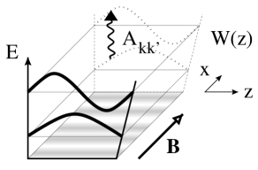
FIG. 7.: Schematic picture of the quantum well. Two exemplary subband wavefunctions are shown. The spatial profile of the impurity potential is sketched on the bottom of the well.

In the absence of an external magnetic field ($B_{\|}=0$), the subbands are uncoupled and, thus, each subband contributes separately to the conductivity. The weak localization correction for a film with $M$ occupied subbands is, therefore, given as

$\displaystyle g_{{\rm WL}}=M\frac{e^{2}}{\pi h}\ln({\tau/\tau_{\phi}}),$

where phase coherent propagation in each subband is limited by the inelastic decoherence time $\tau_{\phi}^{-1}\propto T^{p}$.

An external magnetic field now plays two complementary roles: a) it breaks time-reversal (${\cal T}$) symmetry and b) it couples the different subbands (i.e., if the random disorder potential is $z$-independent, it represents the only possible coupling between subbands). In fact, these two roles are linked: if the subbands remained completely decoupled, ${\cal T}$-invariance of the 2D motion in each of the $M$ subbands would be preserved because the vector potential of the parallel field can be gauged out in each particular subband. The field-induced subband mixing results in a spectrum of effective dephazing rates $1/\tau_{B}^{(k)}$ (where $k=0,\dots,M-1$) with the following properties: at least $M-1$ dephazing rates are quadratic in the magnetic field, $1/\tau_{B}^{(k>0)}\propto B_{\|}^{2}$. The remaining $1/\tau_{B}^{(0)}$ is exactly equal to zero for a ${\cal P}_{z}$-symmetric system whereas it acquires a quadratic field dependence as well if the symmetry is broken (due to an asymmetric confining potential or $z$-dependent impurity scattering). As a result, the field and temperature dependence of the magnetoconductivity are different for a symmetric vs asymmetric confinement potential,

$$g_{\rm WL}(B_{\|},T)=\frac{e^{2}}{\pi h}\left\{\begin{array}[]{cc}p\ln T+2(M-1)\ln B_{\|}&\quad{\rm for}\enspace W(z)=W(-z),\\ 2M\ln B_{\|}&\quad{\rm for}\enspace W(z)\neq W(-z).\end{array}\right.$$ (42)

The derivation of the above weak localization magnetoconductivity formula is most conveniently performed within the non-linear sigma-model formulation that will be presented in chapter VI.

For strong inter-subband impurity scattering, i.e., when the inter-subband scattering rate exceeds the subband splitting at the Fermi level, the weak localization suppression by the in-plane magnetic field happens in the same way as in thin metallic films with diffusive transverse motion, $d\gg\ell$. In a film with diffusive transverse motion, the electron encircles a random flux of order $\Phi\sim B_{\|}d^{2}$ during its diffusive transverse flight, where the time of flight is given as $\tau_{z}\sim d^{2}/D$. While diffusing along the wire for a longer time, $t\gg\tau_{z}$, the electron encircles a random flux with the variance

$\displaystyle\langle\Phi^{2}\rangle\sim\frac{t}{\tau_{z}}\times(B_{\|}d^{2})^{2}=tD(B_{\|}d)^{2},$

which results in a field-induced phase breaking at the rate [22]

$$\tau_{B}^{-1}\sim D(B_{\|}d)^{2}.$$ (43)

Note that the same geometrical argument is applicable to a thin diffusive wire with cross sectional dimensions $\sim d$ in a magnetic field applied along the wire axis

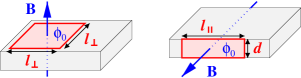
FIG. 8.: Relevant areas for perpendicular and parallel magnetic fields. This admits for estimating field dependence of the respective phase breaking rates, $1/\tau_{B_{\perp}}\sim 1/l_{\perp}^{2}\sim B_{\perp}$ and $1/\tau_{B_{\parallel}}\sim 1/l_{\parallel}^{2}\sim B_{\parallel}^{2}$.

Quantitatively, $\tau_{B}$ can be found from an analysis of the lowest eigenvalue of the Cooperon propagator. The Cooperon propagator is defined by the (diffusion) equation

$\displaystyle\left\{D(i\nabla_{\bf r}-2{\bf A}({\bf r}))^{2}+\frac{1}{\tau_{\phi}}\right\}{\cal C}({\bf r},{\bf r}^{\prime})=\delta({\bf r}-{\bf r}^{\prime})$

with the boundary condition

$\displaystyle\left(\nabla_{{\bf n}}+2i{\bf A}\cdot{\bf n}\right){\cal C}=0.$

Choosing the gauge ${\bf A}=B_{\|}z{\bf e}_{y}$, one can separate variables in the eigenfunction equation for the Cooperon modes,

$\displaystyle-D\left[\frac{\partial^{2}}{\partial z^{2}}-Q_{x}^{2}-\left(Q_{y}-2{B_{\|}z}\right)^{2}\right]\phi_{k,{\bf Q}}(z)=\Omega_{k,{\bf Q}}\phi_{k,{\bf Q}}(z),$

and find the lowest eigenvalue $\Omega_{0,{\bf Q}}=DQ^{2}+\tau_{B}^{-1}$ within perturbation theory. This yields the magnetic decoherence rate [22]

$\displaystyle\tau_{B}^{-1}=\frac{1}{3}D(B_{\|}d)^{2}$

which can be substituted into the weak localization formula for a diffusive film. A similar calculation gives $\tau_{B}^{-1}=D(B_{\|}d)^{2}/8$ for a circular diffusive wire with diameter $d$.

C In-plane magnetoresistance in pure metallic films and quantum magnetoresistance in quasi-ballistic wires with rough edges.

For a clean metallic film or wire, where the dominant scattering processes involve surface or edge roughness, the estimate of $\tau_{B}$ given in Eq. (43) is incorrect due to the exact geometrical phase cancellation described in [23]. Thus, a magnetic field $B_{\|}$ cannot affect the interference pattern, i.e., neither WL magnetoresistance nor magneto-fingerprints are to be expected in these systems at any orientation of the magnetic field. As a result, magnetic field effects acquire several unusual features.

Here, we consider a quasi-ballistic wire with width $d$ and length $L$. In such a wire, a diffusive path may contain ballistic segments with length $\eta=d/\sin\alpha$ much longer than the typical length scale $d$, crossing the wire at the small angle $\alpha$. These segments appear with the probability

$\displaystyle\rho(\eta)\sim\pi^{-1}\left|\frac{d\eta(\alpha)}{d\alpha}\right|^{-1}\sim\eta^{-2},$

for $L>\eta\gg d\gg\lambda_{{\rm F}}$. Thus, the mean free path $\ell$ in such a wire exceeds the width of the wire by a large logarithmic factor, $\ell\sim\langle\eta\rangle\sim d\,\ln(L/d)$.

Quantum in-plane magnetoresistance in such a wire may appear only due to a curving of the longest ballistic paths by the field itself. The effect of this curving leads to a switching of the longest segments between the edges of the wire (or surfaces of a film) and, thus, to a sudden suppression of the interference contribution from paths including these longest ballistic flights. However, the change in the weak localization part of the conductivity in such a situation is overcome by the change in the classical part of the conductivity: due to the cyclotron curving of free electron trajectories in combination with the finite width of the wire, the longest ballistic flights are suppressed, i.e., $\eta<\sqrt{r_{c}d}$ – yielding a mean free path $\ell(B_{\|})\sim\frac{1}{2}d\ln(r_{c}/d)$, where $r_{c}=p_{{\rm F}}/B_{\|}$. Thus, the shortening of the longest ballistic flights happens simultaneously with their involvement into phase accumulation, immediately bringing in a large time-irreversible phase of order of the total flux penetrating through the entire sample. On the other hand, paths that encircle a large flux can participate in the formation of a random interference pattern. Therefore, starting from the field value $B_{{\rm defl}}=\phi_{0}d/(L^{2}\lambda_{{\rm F}})$ (implying $\sqrt{r_{c}d}<L$) – that coincides with the set in of a classical (positive) magnetoresistance – the quantum conductance should acquire a universal random dependence on the field with a characteristic scale related to a flux change of order of the flux quantum. By the same reason, the magnetic field effect on the localization properties of quasi-ballistic wires is opposite to the commonly expected crossover between orthogonal and unitary symmetry classes, i.e., the magnetic field tends to shorten the localization length in a quasi-ballistic wire.

These qualitative expectations have been verified numerically in Ref. [25]. The results of Ref. [25] are based upon the numerical solution of a two-dimensional Anderson Hamiltonian on a square lattice, $H=\sum_{i}|i\rangle\epsilon_{i}\langle i|-V\sum_{\langle ij\rangle}|i\rangle\langle j|$, where $\langle ij\rangle$ denotes nearest neighbor sites $i$ and $j$. The structure considered consists of two ideal leads attached to a scattering region that is $W$ sites wide and $L$ sites long (all lengths are in units of the lattice constant $a$). For simulating bulk disorder, the energies $\epsilon_{i}$ in the scattering region are taken uniformly from the interval $-U/2<\epsilon_{i}-\epsilon_{0}<U/2$, where $U$ is the disorder strength. For sites on the boundary, $\epsilon_{i}=\epsilon_{0}+\epsilon_{B}$ with $\epsilon_{B}=10^{4}$. The rough structure of the boundary was generated by having an equal probability of either 0, 1 or 2 sites at each edge with on-site potential $\epsilon_{0}+\epsilon_{B}$. To simulate the effect of a magnetic field, a Peierls phase factor has been incorporated into $V$ in the scattering region.

FIG. 9.: (a) Distribution function $P(L/\xi)$ for 4 quasi-ballistic samples with $W=$15 and $L=$52(A), 104(B), 208(C) and 416(D) and for a wire (U) with on-site bulk disorder $U=2.0$ (nominal mean free path $\ell\approx 8.5$, $W=15$ and $L=52$). (b) Distribution function $P(g)$ for the two quasi-ballistic structures A and C. (c) $E_{\rm Th}(L)$ for quasi-ballistic wires with $\epsilon_{0}\in[1.5,1.7]$ (circles) and $\epsilon_{0}\in[1.0,1.2]$ (diamonds) and for a wire from the $U$ series (squares). Also shown is the analytical result (cf. Eq. (44) with $hv_{\rm F}=12.3$ and $W=9.3$ (solid curve). The dashed curve corresponds the ergodic law $E_{\rm Th}\sim hD/L^{2}$ with $hD=62.5$.

The effect of Lévy flights has been identified in the numerical results in several ways. One was to study the distribution of transmission coefficients through the wire and the distribution $P(\xi^{-1})$ of the corresponding Lyapunov exponents $\xi^{-1}$. This is shown in Fig. 9(a) (taken from Ref. [25]) for 4 series of quasi-ballistic wires (A-D) as well as a series of samples with bulk ‘defects’ (U). As pointed out by Tesanovich et al [50] and verified numerically in Ref. [51], the length of Lévy flights in quantum systems is limited. The limitation is due to the fact that the uncertainty in the transverse momentum, $\delta k_{\perp}\sim 1/d$, in a wire with a finite width sets a quantum limit to the angles $\alpha\sim d/\eta$ which can be assigned to a classically defined ballistic segment, namely $\alpha>\delta\alpha\sim\delta k_{\perp}/k_{{\rm F}}\sim\lambda_{\rm F}/d$. This sets the cut-off $\eta_{{\rm max}}=d^{2}/\lambda_{{\rm F}}$ and entails a finite localization length $L_{c}\sim\eta_{{\rm max}}$. Samples from the series A and B meet the criterion $L<L_{c}$ which manifests itself in the distribution of Lyapunov exponents by a pronounced peak at small $\xi^{-1}$ corresponding to eigenvalues $T_{n}\approx 1$. This should be compared to the plateau-like distribution [52] obtained in a sample from the series U using the same numerical procedure. Note the finite width of the ballistic peak in $P(\xi^{-1})$ and that $P(0)=0$. The enhanced density of small $\xi^{-1}$ can be identified even in samples from the series C and D with $L\approx L_{{c}}$. In these samples, $P(\xi^{-1})$ starts to show a periodic modulation specific to the localized regime, where the spectrum of Lyapunov exponents tends to crystallize [53, 54].

The distribution of eigenvalues of the transmission matrix results in a finite-width distribution of conductances and, hence, conductance fluctuations. The statistics of conductance fluctuations, $P(g)$, for wires with edge disorder is shown in Fig. 9(b): the results of numerical simulations [25] are plotted for series A, where $\langle g\rangle\approx 2.0$ and the distribution is almost Gaussian, and series C, where $\langle g\rangle\approx\,0.71$. (The conductance is expressed in quantum units $e^{2}/h$.) The distribution function $P(g)$ is the result of the analysis of various realizations of disorder. When calculating correlation functions, there is an additional averaging over energy, since the energy dependence of conductance fluctuations is random on the scale of the Thouless energy $E_{{\rm Th}}$. The latter can be determined from the wire conductance as $g\sim E_{{\rm Th}}(L)/\Delta(L)$, where $\Delta$ is the mean level spacing in the wire. Taking into account the logarithmic multiplier in the dependence of the classical conductance on sample length due to the Lévy flights, one obtains

$$g\sim\frac{e^{2}}{h}\frac{d^{2}}{L\lambda_{{\rm F}}}\ln(\frac{L}{1.7d}).$$ (44)

This result for the wire conductance implies an anomalous scaling of the Thouless energy, $E_{{\rm Th}}=\pi dv_{{\rm F}}L^{-2}\ln(\frac{L}{1.7d})$, with the length of the wire. In Fig. 9(c), it is shown that, indeed, the Levy flights manifest themselves in the correlation energy of UCF in the quasi-ballistic regime. For comparison, it is demonstrated that the results for bulk-disordered samples (U) coincide with the standard scaling law $E_{{\rm Th}}(L)\sim L^{-2}$.

FIG. 10.: (a) Conductance for a quasi-ballistic wire (solid curve) from the B series and a disordered wire (dashed curve) with mean free path $\ell\approx 16$. (b) Variance ${\rm var}(g(B))$ for quasi-ballistic wires from the $B$ series and disordered wires.

Coming now to the magnetic field effects. The expected deflection of Lévy flights at $B>B_{{\rm defl}}$ entailing a break of geometrical flux cancellation is observable in Fig. 10 as pronounced magnetoconductance fluctuations $\delta g(B)=g(B)-\langle g\rangle$ beginning together with a gradual decrease of the average conductance value – which is a purely classical effect. Their variance corresponds to the usual UCF value, and the auto-correlation function as a function of magnetic field gives the correlation field $B_{c}$ corresponding to a change of magnetic flux through the sample area of order $2.5\phi_{0}$ as compared to $1.5\phi_{0}$ in the bulk-disordered case. This seems to explain an earlier experimental observation of UCF in quasi-ballistic semiconductor wires [55].

FIG. 11.: (a) The ensemble averaged conductance as a function of magnetic field for wires from the A and B series. (b) The same curves (A-D) as in Fig. 9(b), but at finite magnetic field $B=0.02\phi_{0}/a^{2}$. (c) The localization length for quasi-ballistic wires (solid curve) and disordered wires (dashed curve) with mean free path $\ell\approx 8.5$.

Furthermore, Fig. 11 shows the tendency of the localization length in a quasi-ballistic wire to increase with the magnetic field – as opposed to the behavior of $L_{{c}}(B)$ in systems with diffusive transverse motion [41, 53]. The relevant field scale at which the localization length in quasi-ballistic wires starts to shorten, $B_{c}\sim\phi_{0}\lambda_{{\rm F}}/W^{3}$, can be obtained from $B_{{\rm defl}}$ by replacing the sample length $L$ with $L_{{c}}$. Formally, this yields a similar field scale as the one leading to a crossover in $L_{{c}}$ between two symmetry classes due Aharonov-Bohm type phase effects. Thus, the latter is hindered by the deflection effect and does not appear as an intermediate crossover regime.

IV In-plane magnetoresistance due to spin-orbit coupling

A Spin-orbit coupling in 2D heterostructures and quantum dots

Coupling between the electron spin and its orbital motion is a relativistic effect inherent to many metallic and semiconductor systems. For example, in zinc-blend type III-V semiconductors, such as GaAs, which have no inversion symmetry in the unit cell, the 3D bulk dispersion of conduction band electrons contains terms that are cubic in the electron momentum and linear in its spin operator [56]. This generates a linear spin-orbit coupling for electrons confined to the 2D plane in a heterostructure or a quantum well [57, 58],

$$H_{0} = \frac{{\bf p}^{2}}{2m}+\frac{\alpha_{{\sc br}}}{2m}[{\bf p\times e}_{z}]\cdot{\underline{\sigma}}+\frac{\alpha_{{\rm cr}}}{2m}(p_{x}{\sigma_{x}}{}-p_{y}{\sigma_{y}}{})=\frac{{\bf p}^{2}}{2m}+\frac{v_{\rm F}}{2\lambda_{{\rm SO}}}{\bf n}_{\bf p}\cdot\underline{\sigma},$$ (45)

where ${\bf n}_{\bf p}$ characterizes the direction and frequency of spin precession (of an electron moving with momentum ${\bf p}$) measured in units of $v_{\rm F}/\lambda_{\rm SO}$, where $1/\lambda_{\rm SO}=\sqrt{\alpha_{{\sc br}}^{2}+\alpha_{{\rm cr}}^{2}}$.

The form of the spin-orbit (SO) coupling in Eq. (45) is specified for a GaAs heterostructure grown along the (001) plane which has the symmetry of a square lattice without inversion symmetry within the unit cell. It includes two possible combinations of spin and momentum operators that are invariant under the symmetry transformation corresponding to such a lattice symmetry, parameterized by two constants, $\alpha_{\sc br}$ (the so-called Bychkov-Rashba term) and $\alpha_{\rm cr}$ (the crystalline anisotropy term).

For a particle moving diffusively in an infinite heterostructure, spin-orbit coupling provides an efficient mechanism for spin relaxation. In the frame of the moving electron, its spin undergoes a precession with angular frequency $\underline{\Omega}\sim{\bf n}_{\bf p}v_{\rm F}/\lambda_{{\rm SO}}$ which randomly changes direction each time the particle changes its direction of propagation due to scattering at impurities. Using the parameterization of the SO coupling by a spin-orbit length $\lambda_{{\rm SO}}$, as in Eq. (45), the precession angle acquired between successive scattering events can be estimated as $\delta\varphi_{\rm so}\sim\tau v_{\rm F}/\lambda_{{\rm SO}}=\ell/\lambda_{{\rm SO}}$. For weak SO coupling, $\ell/\lambda_{{\rm SO}}\ll 1$, the electron spin precession can be viewed as a random walk of the electron spin polarization vector around the unit sphere with a typical step size $\delta\varphi_{\rm so}$. This causes a loss of spin memory at the (Dyakonov-Perel) rate [26]

$$\tau_{{\rm DP}}^{-1}\sim D/\lambda_{{\rm SO}}^{2}.$$ (46)

In a 2D electron gas, this parameter limits the diffusion time in the triplet Cooperon channel (whereas the singlet Cooperon channel is unaffected). Therefore, it suppresses the triplet contribution to the weak localization correction formula and controls the crossover between the weak localization (at weak SO coupling) and weak anti-localization (at strong SO coupling) regimes in the quantum correction to the conductivity [27, 28].

When the electron motion within the 2D plane is also confined laterally, the use of the so called Dyakonov-Perel formula, Eq. (46), dramatically overestimates the rate of spin relaxation. In particular, if the electron motion is confined to a single 1D channel (i.e., a quantum wire), no real spin relaxation takes place – despite the electron spin precession. In this case, the spin precession is a reversible process that rotates the initial electron spin to the same definite state at each point along the wire, no matter how many times the electron moves forwards and backwards. Mathematically, the above-mentioned property of the SO coupling becomes transparent in the following way: Consider a one-dimensional electron moving, say, along the $x$-direction. Applying the unitary transformation,

$\displaystyle U=\exp\left(\frac{ix}{2\lambda_{{\rm SO}}}{\bf n}({\bf l}_{x})\cdot\underline{\sigma}\right),$

where ${\bf l}_{x}$ is a unit vector along the wire axis, the SO coupling is eliminated completely from the electron dispersion represented in a rotated spin-coordinate frame [59, 60]. Therefore, it does not affect any charge transport properties. By contrast, the Dyakonov-Perel relaxation of the spin of a 2D electron (with the rate described in Eq. (46)) is the result of the diversity of paths the electron may use to move between two points in the sample.

A small quantum dot with dimensions $L\ll\lambda_{{\rm SO}}$ represents an intermediate situation between the 1D and the 2D system as described above. Here, we shall consider a dot coupled to metallic leads via two contacts, left ($l$) and right ($r$), each with $N_{l,r}\gtrsim 1$ open orbital channels. Then the escape rate [30] from the dot into the leads is given as

$\displaystyle\gamma\equiv\tau_{\rm esc}^{-1}=(N_{l}+N_{r})\Delta/(2\pi),$

where $\Delta=2\pi/(m{\cal A})$ is the mean level spacing (${\cal A}$ area of the dot).

Although there is no unitary transformation that eliminates the SO coupling completely by changing to a locally rotated spin coordinate system, the linear term in the small SO coupling constant can be cancelled by a proper spin-dependent gauge transformation [31], thus, generating only contributions to the free electron Hamiltonian of order $\lambda_{{\rm SO}}^{-2}$ (or higher). As a result, the influence of spin-orbit coupling on the transport characteristics of a small dot is suppressed as compared to the infinite 2D system with similar material parameters.

However, the application of an in-plane magnetic field changes the situation. The transformation to the locally rotated spin-coordinate frame turns an initially constant external magnetic field, ${\bf B}=B\,{\bf l}$, into an inhomogeneous Zeeman field that accelerates the loss of spin memory of an electron passing through the dot. Below, this effect will be described quantitatively.

For the sake of convenience, we choose the coordinate system ($x_{1},x_{2}$) with axes along the crystallographic directions ${\bf e}_{1}=[110]$ and ${\bf e}_{2}=[1\bar{1}0]$ such that we can exploit the $C_{2v}$ lattice symmetry of the (001) plane of GaAs. Then, the single-particle Hamiltonian in the presence of an in-plane magnetic field ${\bf B}=B\,{\bf l}_{\parallel}$ with ${\bf l}_{\parallel}=(l_{1},l_{2},0)$ can be rewritten as

$$H_{0}=\frac{1}{2m}\left[\left(p_{1}-\frac{\sigma_{2}}{2\lambda_{1}}\right)^{2}+\left(p_{2}+\frac{\sigma_{1}}{2\lambda_{2}}\right)^{2}\right]+\frac{\epsilon_{{\rm Z}}}{2}\,{\bf l}_{\parallel}\cdot\underline{\sigma},$$ (47)

where $\lambda_{1,2}=1/(\alpha_{\sc br}\pm\alpha_{\rm cr})$ characterize the length scales associated with the strength of the SO coupling for electrons moving along the principal crystallographic directions. Here, $\sigma_{1,2,3}$ are Pauli matrices with $\sigma_{2}=-\sigma_{2}^{T}$ and $\sigma_{1,3}=\sigma_{1,3}^{T}$. $\epsilon_{Z}=g\mu_{B}B_{\parallel}$ is the Zeeman energy associated with the parallel magnetic field. Furthermore, ${\bf p}={\bf P}-{\bf A}$ is the kinetic momentum with ${\bf P}=-i\nabla$ and the vector potential ${\bf A}=B_{z}[{\bf r\times e}_{z}]/2$ corresponding to an additional perpendicular magnetic field.

In the following, we assume the dot to be sufficiently small to fulfill the conditions $L_{1,2},\ll\lambda_{1,2}$ and $\gamma,\epsilon_{{\rm Z}}\ll E_{{\rm Th}}$, where $E_{{\rm Th}}=hD/L^{2}$ is the Thouless energy.

B Effect of spin-orbit coupling on weak localization and conductance fluctuations

For a spin-$\frac{1}{2}$ particle in a quantum dot connected to adiabatic ballistic contacts, the WL corrections to the conductance can be related to the lowest-lying modes of Cooperons in the singlet and triplet channels. The expressions for the different Cooperon modes can summarized in the equation

$${\cal C}^{LM}=\frac{1}{2}\left\langle{\rm tr}\left[\sigma_{L}\sigma_{2}\hat{G}_{R}^{T}(\varepsilon)\sigma_{2}\sigma_{M}\hat{G}_{A}(\varepsilon-\omega)\right]\right\rangle,$$ (48)

where $L,M=0,\dots,3$. Note that the use of the (perturbative) diagrammatic technique in the description of quantum dots is justified if the number of channels in the leads is large, $N_{l,r}\gg 1$.

In the absence of SO coupling and Zeeman splitting, the Cooperon modes ${\cal C}^{LM}$ can be separated into four completely independent channels, i.e., one singlet channel ${\cal C}_{0}={\cal C}^{00}$ and three triplet channels ${\cal C}_{1}^{M}={\cal C}^{MM}$ ($M=1,2,3$). Or, in a matrix representation ,

$\displaystyle\hat{{\cal C}}={\cal C}\hat{\delta},\qquad{\rm where}\enspace\hat{\delta}\equiv\delta_{LM},$

and ${\cal C}$ obeys the conventional diffusion equation. This leads to the familiar result for the WL corrections [27],

$\displaystyle g^{{\rm WL}}\propto\frac{e^{2}}{h}\left({\cal C}_{0}-\sum_{M=1,2,3}{\cal C}_{1}^{M}\right).$

However, the SO coupling and Zeeman splitting mix the various components [28] and, thus, split their spectra. This changes the conventional diffusion equation into the matrix equation

$$\hat{\Pi}\,\hat{{\cal C}}({\bf x},{\bf x}^{\prime})=\delta({\bf x}\!-\!{\bf x}^{\prime})\,\hat{\delta},$$ (49)

where

$$\hat{\Pi} = -D\left((\partial_{x_{1}}+2iA_{1})\hat{\delta}-\frac{i}{\lambda_{1}}\hat{S}_{2}\right)^{2}-D\left((\partial_{x_{2}}+2iA_{2})\hat{\delta}+\frac{i}{\lambda_{2}}\hat{S}_{1}\right)^{2}+\gamma\,\hat{\delta}+i\epsilon_{{\rm Z}}\,\hat{\eta}.$$ (50)

Here, $\hat{S}_{K}^{LM}=-i\varepsilon^{KLM}$ are spin-1 operators ($K,L,M=1,2,3$ ), and $\varepsilon^{KLM}$ is the antisymmetric tensor. As a $4\times 4$ matrix, $\hat{S}$ also has zero elements when $L=0$ or $M=0$. The other relevant matrix $\hat{\eta}$ is defined as

$\displaystyle\eta^{LM}=l_{L}\,\delta_{0M}+l_{M}\,\delta_{0L}$

(where $l_{K}$ is the $K$th component of ${\bf l}_{\parallel}$) indicating that coherence between electrons with opposite polarization is lost on the time scale $\epsilon_{{\rm Z}}^{-1}$.

Eq. (50) is supplemented with a boundary condition at the edge of the dot characterized by the normal direction ${\bf n}_{\parallel}=(n_{1},n_{2})$,

$$\left[{\bf n}_{\parallel}\cdot(\nabla+2i{\bf A})\hat{\delta}-in_{1}\lambda_{1}^{-1}\hat{S}_{2}+in_{2}\lambda_{2}^{-1}\hat{S}_{1}\right]\hat{{\cal C}}=0.$$ (51)

Because of the boundary condition, the lowest mode of the Cooperon cannot be a mere constant solution, such as ${\bf q}=0$. To find the lowest Cooperon mode in this problem, one should make such a gauge transformation (that is, a unitary rotation of the Cooperon spin components)

$\displaystyle\hat{{\cal C}}=\hat{U}\hat{\cal C}^{\prime}\hat{U}^{-1},$

that would transform the original boundary condition into ${\bf n}_{\parallel}\cdot\nabla\hat{\cal C}^{\prime}=0$. In the new spin coordinate system, one can now approximate the lowest Cooperon mode for $\hat{\cal C}^{\prime}$ by a ${\bf q}=0$ solution, i.e., $\hat{\cal C}^{\prime}={\rm const.}$, and evaluate its eigenvalue using the standard methods of the Hamiltonian perturbation theory with respect to the terms generated by such a rotation in the initial differential operator $\hat{\Pi}$. This program can be realized by applying the transformation

$\displaystyle\hat{U}=\exp\left[i\left(\frac{x_{2}}{\lambda_{2}}\hat{S}_{1}-\frac{x_{1}}{\lambda_{1}}\hat{S}_{2}\right)\right]\exp[-i\varphi_{s}({\bf x})\hat{S}_{3}]\exp[-i\varphi_{a}({\bf x})],$

where function $\varphi=\varphi_{s}+\varphi_{a}$ transforms from the symmetric gauge to a gauge, where the normal component of the vector potential at the boundary of the dot vanishes. This eliminates the lowest orders SO coupling terms from the boundary condition, and, thus, (in a small dot, $L_{1,2}\ll\lambda_{1,2}$) can be followed by a perturbative analysis of extra terms in Eq. (50) generated by the rotation $\hat{U}$. This results in the 0D matrix equation for the Cooperon,

$$\hat{{\cal C}}=\!\left[\gamma\hat{\delta}+i\epsilon_{{\rm Z}}\hat{\eta}+\!\left(\frac{1}{\sqrt{\tau_{B}}}\hat{\delta}-\!\sqrt{\epsilon_{\bot}^{{\rm so}}}\hat{S}_{3}\right)^{2}\!\!+\epsilon_{\bot}^{{\rm Z}}(\hat{\delta}\!-\!\hat{S}_{3}^{2})+\epsilon_{\parallel}^{{\rm so}}(\hat{\bf S}^{2}\!-\!\hat{S}_{3}^{2})\right]^{-1}\!\!\!\!\!\!,$$ (52)

which depends on six different energy scales to be discussed in the following. ($\gamma$ and $\epsilon_{Z}$ have been introduced earlier.)

In Eq. (52), the two parameters

$$\tau_{B}^{-1}=\frac{4\pi B_{z}^{2}}{\Delta}\left\langle|M_{\alpha\beta}|^{2}\right\rangle=\kappa E_{{\rm Th}}(2eB_{z}{\cal A})^{2},\qquad\qquad\qquad\epsilon_{\bot}^{{\rm so}}=\kappa E_{{\rm Th}}\left({\cal A}/\lambda_{1}\lambda_{2}\right)^{2},$$ (53)

possess the same dependence on the shape of the dot and the disorder in the sample. Here, $\kappa$ is a geometry-dependent coefficient. Furthermore, the random quantities $M_{\alpha\beta}$ are the non-diagonal matrix elements of the magnetic moment of the electron in the dot. Note that the difference in the third term in brackets of Eq. (52), containing $\tau_{B}^{-1}$ and $\epsilon_{\bot}^{{\rm so}}$, reflects the addition or subtraction of the Berry and Aharonov-Bohm phases, as was pointed out in Ref. [59, 60].

The parameter $\epsilon_{\bot}^{{\rm Z}}$ in Eq. (52) is the result of a parallel field induced additional Zeeman splitting,

$$\epsilon_{\bot}^{{\rm Z}}=\frac{\epsilon_{Z}^{2}}{2\Delta}\sum_{i,j=1,2}\frac{l_{i}l_{j}}{\lambda_{i}\lambda_{j}}L_{i}L_{j}\;\Xi_{ij},\qquad{\rm where}\enspace\Xi_{ij}=\frac{\pi}{L_{i}L_{j}}\langle X_{i}^{\alpha\beta}X_{j}^{\beta\alpha}\rangle,$$ (54)

and $x_{1,2}^{\alpha\beta}$ are the non-diagonal matrix elements of the dipole moment of the electron in the dot. The quantities $\Xi_{ij}$ depend on geometry and the disorder and may be estimated as $\Xi\simeq\Delta/E_{{\rm Th}}=g^{-1}$. This yields $\epsilon_{\bot}^{{\rm Z}}\ll\epsilon_{{\rm Z}}$. A similar energy scale has been found in other recent publications [61].

Finally, the parameter

$$\epsilon_{\parallel}^{{\rm so}}\sim\left[\left(L_{1}/\lambda_{1}\right)^{2}+\left(L_{2}/\lambda_{2}\right)^{2}\right]\epsilon_{\bot}^{{\rm so}}\ll\epsilon_{\bot}^{{\rm so}}$$ (55)

introduces the smallest energy scale through which the SO coupling affects the Cooperon propagator.

In principle, the form of Eq. (52) is applicable beyond the diffusive approximation as it follows purely form symmetry considerations. Now, the weak localization corrections can be found from Eq. (52) as

$$g^{{\rm WL}}\propto{\rm tr}\left[\,\hat{{\cal C}}\left(\hat{\delta}-{\hat{\bf S}^{2}}\right)\right].$$ (56)

In the absence of a perpendicular magnetic field ($\tau_{B}^{-1}=0$) and using the assumptions made above, namely $\gamma,\epsilon_{{\rm Z}},D/\lambda_{1,2}^{2}\ll E_{{\rm Th}}$, this yields

$$g^{{\rm WL}}\approx\frac{e^{2}}{h}\frac{a_{lr}}{4}\left(-\frac{\gamma}{\gamma+\epsilon_{\bot}^{{\rm so}}}-\frac{\gamma}{\gamma+\epsilon_{\bot}^{{\rm Z}}+2\epsilon_{\parallel}^{{\rm so}}}+\frac{\epsilon_{\bot}^{{\rm so}}}{\gamma+\epsilon_{\bot}^{{\rm so}}+\frac{\epsilon_{{\rm Z}}^{2}}{\gamma}}\right),$$ (57)

where the fact that $\epsilon_{\bot}^{{\rm Z}}\ll\epsilon_{{\rm Z}}$ has been used. Furthermore, we introduced the notation

$\displaystyle a_{lr}=\frac{4N_{l}N_{r}}{(N_{l}+N_{r})^{2}}.$

The formula in Eq. (57) describes the average tendency of the in-plane magnetoresistance of a dot due to the interplay between SO coupling and Zeeman splitting.

It is interesting to note that the application of a Zeeman field (i.e., an in-plane magnetic field [3]) alone does not suppress the weak localization corrections completely as long as $\epsilon_{{\rm Z}}\ll E_{{\rm Th}}$ – whereas in the opposite case, $\epsilon_{{\rm Z}}\gtrsim E_{{\rm Th}}$, it does. However, the orbital effect of such a strong in-plane field is already sufficient to suppress weak localization as discussed in the previous section.

In the regime $\epsilon_{\parallel}^{{\rm so}}/\gamma,\epsilon_{\bot}^{{\rm so}}/\gamma\rightarrow 0$ relevant for the experiments on small dots [3], the form of Eq. (57) is dominated by the first two terms,

$$g^{{\rm WL}}(B)\approx-\frac{e^{2}}{h}\frac{a_{lr}}{4}\left(1+\frac{1}{1+\epsilon_{\bot}^{{\rm Z}}(B)/\gamma}\right).$$ (58)

This suggests a possible procedure for measuring the ratio $\lambda_{1}/\lambda_{2}$. By fitting the experimental magnetoresistance data to $g^{{\rm WL}}(B)$, one can determine the characteristic in-plane magnetic field ${\cal B}$ at which the weak localization part of the dot conductance gets suppressed by the factor of two. For a dot with a strongly anisotropic shape, this parameter would depend on the orientation of the in-plane magnetic field. In particular, ${\cal B}$ should be measured for two orientations of the in-plane field: namely ${\cal B}_{[110]}$ for ${\bf l}=[110]$ and ${\cal B}_{[1\bar{1}0]}$ for ${\bf l}=[1\bar{1}0]$. Furthermore, one should perform a simultaneous measurement of the two characteristic fields ${\cal B}_{[110]}^{\prime}$ and ${\cal B}_{[1\bar{1}0]}^{\prime}$ in a dot produced on the same chip by rotating the same lithographic mask by 90^∘. The anisotropy of the SO coupling is then obtained directly from the ratio

$\displaystyle\left({\cal B}_{[110]}{\cal B}_{[110]}^{\prime}/{\cal B}_{[1\bar{1}0]}{\cal B}_{[1\bar{1}0]}^{\prime}\right)=\left(\lambda_{1}/\lambda_{2}\right)^{4},$

that is, independently of details of the sample geometry.

The results for weak localization part of a two-terminal conductance of a dot and the variance of its universal fluctuations are summarized for the limiting regimes in the following equation,

$$g^{{\rm WL}}=-\,\frac{2-\beta}{2\beta\Sigma}\,a_{lr}\,\frac{e^{2}}{h},\qquad\langle\delta g^{2}\rangle=\frac{s}{4\beta\Sigma}\,a_{lr}^{2}\left(\frac{e^{2}}{h}\right)^{2}.$$ (59)

Here, the conventional parameter $\beta$ describes time-reversal symmetry of the orbital motion, $s$ is the Kramers’ degeneracy parameter, and $\Sigma$ is an additional parameter characterizing the mixing of states with different spins for strong Zeeman splitting. In a small dot [3], where $\epsilon_{\parallel}^{{\rm so}}/\gamma\rightarrow 0$ as well as $\epsilon_{\bot}^{{\rm so}}/\gamma\rightarrow 0$, one obtains the following values for the different parameters: $\beta=1$ indicates that for weak SO coupling the electron spin splitting cannot violate the time-reversal symmetry of the orbital motion; Kramers’ degeneracy is preserved ($s=2$) for $\epsilon_{{\rm Z}}<\gamma$, but lifted ($s=1$) for $\epsilon_{{\rm Z}}>\gamma$; finally, $\Sigma=1$ for $\epsilon_{\bot}^{{\rm Z}}<\gamma$ and $\Sigma=2$ for $(\epsilon_{{\rm Z}}\gg)\,\epsilon_{\bot}^{{\rm Z}}>\gamma$ at very strong Zeeman splitting.

V In-plane magnetoresistance in systems with magnetic impurities

In addition to a purely potential disorder, metals and semiconductors may contain magnetic impurities [40, 39]. In fact, most of real materials certainly do have them to some extent [62, 63]. In this section, we discuss the influence of a dilute magnetic contamination on the quantum transport characteristics of disordered conductors. In particular, we describe the suppression of weak localization, and its restoration by an in-plane magnetic field due to a polarization of the localized magnetic moments – which slows down the decoherence of conducting electrons and produces an observable magnetoresistance, $g(B_{\|})=g_{{\rm class}}+\delta g^{\rm WL}(B_{\|})$.

A Electron spin relaxation and Korringa time for magnetic impurities

The coupling between a spin-$\frac{1}{2}$ electron and the magnetic impurity spin originates from the exchange interaction and can be described by the Hamiltonian

$\displaystyle\hat{{\cal H}}_{{\rm s}}=J\,\,{\bf S}({\bf r})\cdot\underline{\sigma},$

where ${\bf S}$ is the impurity spin and $J$ is the exchange coupling. Furthermore, $\underline{\sigma}$ is a vector of Pauli matrices. When scattering on a magnetic impurity, the electron can change its spin state. Thus, electrons diffusing in a disordered conductor containing magnetic impurities loose their spin memory after the time scale $\tau_{{\rm s}}$ determined by the spin-flip relaxation rate

$\displaystyle\tau_{{\rm s}}^{-1}\sim\nu\,J^{2}\,S(S+1)\sim\nu\,n_{{\rm s}}\,j^{2}\,S(S+1).$

Here, $j$ the exchange coupling due to a single impurity and $n_{\rm s}$ is the density of magnetic impurities. For dilute magnetic impurities, $\tau_{{\rm s}}\gg\tau$.

To incorporate spin-flip scattering into the quantitative Cooperon/diffuson analysis of weak localization and UCFs, one has to make assumptions concerning correlation properties of this additional source of disorder. Similarly to the non-magnetic impurities, we assume the magnetic disorder to be Gaussian $\delta$-correlated with zero mean and variance

$\displaystyle\langle JS_{\alpha}({\bf r},t)JS_{\beta}({\bf r}^{\prime},t)\rangle=\frac{1}{6\pi\nu\tau_{{\rm s}}}\delta_{\alpha\beta}\,\delta({\bf r}-{\bf r}^{\prime})$

at coinciding moments of time.

There is, however, an important difference between potential disorder, which is static for a fixed configuration of impurities in the sample, and magnetic scatterers, which change their spin state after each electron-impurity spin-flip event. As a result, magnetic disorder has its own dynamics, and a magnetic scatterer forgets about its initial spin state with the so-called Korringa relaxation rate [64]

$$\tau_{{\rm K}}^{-1}\sim\nu\,n_{{\rm e}}\,j^{2}\frac{T}{\epsilon_{{\rm F}}},$$ (60)

where $n_{\rm e}$ is the electron density.

Korringa relaxation, as it is known, takes place due to spin-flip scattering at the impurity of any electron with energy $|\epsilon-\epsilon_{{\rm F}}|\sim T$ close to the Fermi level. Therefore, the corresponding relaxation rate is temperature-dependent, whereas the single-electron spin relaxation rate $1/\tau_{{\rm s}}$ is temperature independent. As a result, for temperatures $T>T_{{\rm s}}$ higher than a certain temperature

$\displaystyle T_{{\rm s}}\sim\frac{n_{{\rm s}}}{n_{{\rm e}}}\epsilon_{{\rm F}},$

an impurity changes its spin state faster than any free electron whose individual propagation we may follow, i.e., $1/\tau_{{\rm K}}>1/\tau_{{\rm s}}$. By contrast, for $T<T_{{\rm s}}$, the single-electron spin relaxation is faster, $1/\tau_{{\rm s}}>1/\tau_{{\rm K}}$, and the exchange field of the impurities can be treated as static when analyzing weak localization effects.

The relaxation of the impurity spin sub-system should be taken into account in the correlation properties of this source of randomness. This can be achieved by saying that, for the same magnetic scatterer,

$\displaystyle\langle S_{\alpha}({\bf r},t)S_{\beta}({\bf r},0)\rangle=\delta_{\alpha\beta}\,S(S+1)\,e^{-|t|/\tau_{{\rm K}}}.$

B Spin-flip scattering, impurity spin dynamics and polarization of impurities in weak localization

After an electron flips its spin a few times at encountered magnetic impurities, the coherence between waves propagating in clockwise and anti-clockwise directions along the same geometrical path is destroyed. In the regime of fast Korringa relaxation, $1/\tau_{{\rm K}}>1/\tau_{{\rm s}}$, this happens since electron waves traveling towards each other along a loop encounter the same magnetic scatterer at different moments of time and, therefore, in uncorrelated initial states. In the regime of slow Korringa relaxation, $1/\tau_{{\rm K}}<1/\tau_{{\rm s}}$, decoherence between these two waves accumulates due to a non-commutativity of electron spin operators, whose product would appear due to the coupling to spin-flip transitions between the same initial and final states of the same set of magnetic impurities visited in the opposite order.

As a result, in a magnetically contaminated conductor, the time of flight along trajectories forming the enhancement of backscattering is limited by the spin-relaxation time, $\tau_{{\rm s}}$. As in the previous section, a quantitative description of weak localization corrections to the conductivity,

$$g^{\rm WL}=\frac{e^{2}}{2\pi h}\int_{\tau}^{\infty}dt\;\left[{\cal C}_{0}(t;0)-3\,{\cal C}_{1}(t;0)\right],$$ (61)

requires a diagrammatic evaluation of the singlet and triplet Cooperon correlation functions. In Eq. (61), the variable of integration $t$ is the difference between moments of time when clockwise and anti-clockwise propagating waves pass through the same point in space. As shown in Fig. 12, when deriving the equation of motion for Cooperons, one should include magnetic impurity scattering into both, (a) the self-energy of the impurity-averaged electron Green functions, i.e., as a correction to the mean free time, and (b) the two-particle correlation functions as additional impurity lines in the ladder diagram. Taking into account the Clebsh-Gordan coefficients that appear upon splitting the Cooperon into singlet and triplet channels, the equation for the Cooperon takes the form

$$\left\{\partial_{t}-D\nabla^{2}+\frac{1}{\tau_{{\rm s}}}\left(1+c_{J}e^{-|t|/\tau_{{\rm K}}}\right)\right\}{\cal C}_{J}(t,t^{\prime};{\bf r},{\bf r}^{\prime})=\delta(t-t^{\prime})\delta({\bf r}-{\bf r}^{\prime}),$$ (62)

where $J=0$ (spin-singlet) or $1$ (spin-triplet), and $c_{0}=1$, $c_{1}=-1/3$. The time-dependence accounts for the fact that, for clockwise and anti-clockwise trajectories, electron waves test the same scatterer at different moments of time. If the relevant time scale determining the value of the integral in Eq. (61) is large such that $|t|>\tau_{{\rm K}}$, the states of the same impurity seen by waves propagating in opposite directions are uncorrelated. In this regime, the solution of Eq. (62) is

$${\cal C}({\bf q},\omega)=\frac{1}{D{\bf q}^{2}-i\omega+\tau_{{\rm s}}^{-1}}\;,$$ (63)

with the same relaxational pole $\tau_{{\rm s}}^{-1}$, i.e., the single-particle spin relaxation rate, in all spin channels. This regime is realized when $\tau_{{\rm K}}<\tau_{{\rm s}}$, that is, at high temperatures $T>T_{{\rm s}}$.

By contrast, for $\tau_{{\rm K}}>\tau_{{\rm s}}$, the integral in Eq. (61) is determined by the behavior of Cooperons at $|t|<\tau_{{\rm K}}$, where the decoherence in the triplet channel takes about thrice longer than in the singlet channel,

$\displaystyle{\cal C}_{0}({\bf q},\omega)=\frac{1}{D{\bf q}^{2}-i\omega+2\tau_{{\rm s}}^{-1}}\;,\;\;{\cal C}_{1}^{\alpha\beta}({\bf q},\omega)=\frac{\delta_{\alpha\beta}}{D{\bf q}^{2}-i\omega+\frac{2}{3}\tau_{{\rm s}}^{-1}}\;.$

The latter feature indicates that a single spin-flip does not completely destroy coherence between clock and anti-clockwise paths, given that in both propagation scenarios the magnetic impurity state undergoes exactly the same transition.

FIG. 12.: Cooperon for $|t|<\tau_{K}$ (both contributions) and $|t|>\tau_{K}$ (only left diagram). (The thin dashed line represent scattering from the non-magnetic impurities while the thick dashed lines stand for (spin-flip) scattering from the magnetic impurities.)

Eq. (62) can be solved using the following substitution,

$\displaystyle{\cal C}_{J}(t,t^{\prime};{\bf r},{\bf r}^{\prime})=e^{-f(t)}\,\tilde{{\cal C}}_{J}(t,t^{\prime};{\bf r},{\bf r}^{\prime})\,e^{\,f(t^{\prime})}\,,$

with

$\displaystyle f(t)=\frac{1}{\tau_{{\rm s}}}\left(t+c_{J}\tau_{{\rm K}}\,{\rm sign}\,t\,(1-e^{-|t|/\tau_{{\rm K}}})\right)\,.$

Then the ‘modified’ Cooperon $\tilde{{\cal C}}_{J}(t,t^{\prime};{\bf r},{\bf r}^{\prime})$ obeys the conventional diffusion equation $(\partial_{t}-D\nabla^{2})\tilde{{\cal C}}_{J}(t,t^{\prime};{\bf r},{\bf r}^{\prime})=\delta(t-t^{\prime})\delta({\bf r}-{\bf r}^{\prime})$. After substituting the resulting expression for the Cooperon ${{\cal C}}_{J}$ back into Eq. (61), we arrive at

$$g^{{\rm WL}}=\frac{e^{2}}{2\pi h}(D\tau_{{\rm s}})^{1-\frac{d}{2}}\int\limits_{\tau/\tau_{{\rm s}}}^{\infty}\frac{d\theta}{\theta^{d/2}}\left\{\exp\left[-2\theta-\frac{2\tau_{{\rm K}}}{\tau_{{\rm s}}}(1-e^{-\theta\tau_{{\rm s}}/\tau_{{\rm K}}})\right]-3\exp\left[-2\theta+\frac{2\tau_{{\rm K}}}{3\tau_{{\rm s}}}(1-e^{-\theta\tau_{{\rm s}}/\tau_{{\rm K}}})\right]\right\}.$$ (64)

In the ‘low-temperature’ limit, where $\tau_{{\rm K}}^{-1}\rightarrow 0$,

$$g^{{\rm WL}}(\tau_{{\rm K}}^{-1})\rightarrow 0=-\frac{e^{2}}{\pi h}(D\tau_{{\rm s}})^{1-\frac{d}{2}}\left\{\begin{array}[]{cc}{\frac{\pi}{\sqrt{2}}(3^{3/2}-1)}&\qquad d=1,\\ {\ln\frac{3^{3/2}\tau_{{\rm s}}}{4\tau}}&\qquad d=2.\end{array}\right.$$ (67)

For comparison, in the limit $\tau_{{\rm K}}^{-1}\rightarrow\infty$, the above equation changes into

$$g^{{\rm WL}}(\tau_{{\rm K}}^{-1}\rightarrow\infty)=-\frac{e^{2}}{\pi h}(D\tau_{{\rm s}})^{1-\frac{d}{2}}\left\{\begin{array}[]{cc}\sqrt{\frac{\pi}{2}}&\qquad d=1,\\ {\ln\frac{\tau_{{\rm s}}}{\tau}}&\qquad d=2.\end{array}\right.$$ (70)

The difference between the dynamic and static results in Eqs. (70) and (67) manifests itself in a weak temperature dependence of the conductivity,

$$\sigma(T>T_{{\rm s}})-\sigma(T\ll T_{{\rm s}})\approx\frac{e^{2}}{2\pi h}(D\tau_{{\rm s}})^{1-\frac{d}{2}}\left\{\begin{array}[]{cc}{1.2}&\qquad d=1,\\ 1.9&\qquad d=2.\end{array}\right.$$ (73)

So far in this section, we addressed only the suppression of weak localization by spin-flip scattering, whereas our main goal was to identify possible effects of an external magnetic field leading to an observable in-plane magnetoresistance. An in-plane magnetic fields tends to polarize the paramagnetic impurities, thus, opening a gap $\epsilon_{{\rm Z}}^{{\rm(imp)}}=g^{{\rm(imp)}}\mu_{{\rm B}}B_{\parallel}$ for the electron spin-flip relaxation process. At high magnetic fields, $\epsilon_{{\rm Z}}^{{\rm(imp)}}\gtrsim T$, the allowed electron energies are insufficient to flip the impurity spin, i.e., spin-flip scattering is suppressed. Thus, at $B_{\parallel}>B_{{\rm s}}$, where

$$B_{{\rm s}}(T)=T/(g^{{\rm(imp)}}\mu_{{\rm B}}),$$ (74)

magnetic impurities act as non-magnetic ‘potential’ scatterers, with the only difference that their potential profiles are different for spin-$\uparrow$ and spin-$\downarrow$ electrons. Treating the spin-$\uparrow$ and spin-$\downarrow$ electron subsystems separately, one may conclude that, for $T\ll\epsilon_{{\rm Z}}^{{\rm(imp)}}$, each of them contributes a ‘restored’ value towards the weak localization correction to the conductivity (conductance), which results in its overall drop across a broad range of in-plane magnetic fields,

$$g(B_{\parallel}\gg B_{{\rm s}})-g(B_{\parallel}=0)\sim-\,\frac{e^{2}}{\pi h}\times\left\{\begin{array}[]{cl}\ln{\displaystyle\frac{\tau_{\varphi}}{\tau_{s}}},&\qquad{\rm 2D;}\\ \sqrt{{\displaystyle\frac{1}{D\tau_{s}}}}&\qquad{\rm Q1D\enspace wire;}\\ 1&\qquad{\rm 0D\enspace dot.}\end{array}\right.$$ (78)

In Eq. (78), $\tau_{\varphi}>\tau_{{\rm s}}$ is a ‘true’ inelastic decoherence rate due to the electron-electron interaction or external electromagnetic noise.

The quantitative analysis of a system with fully polarized static magnetic impurities implies the evaluation of all Cooperon channels, ${\cal C}_{0}$, ${\cal C}_{10}$, and ${\cal C}_{1\pm 1}$. The first two happen to have a gap in the spectrum, both due to i) the splitting between up/down-spin bands caused by the combination of $B_{\parallel}$ and the mean exchange splitting due to impurities, and ii) the difference between the scattering conditions for up/down-spin electron. By contrast, ${\cal C}_{11}$ and ${\cal C}_{1-1}$ remain massless. When $\tau_{\varphi}\gg\tau_{{\rm s}}$, the crossover between the two limits in Eq. (78) can be roughly described by substituting the electron spin-flip rate at intermediate fields,

$$\tau_{{\rm s}}^{-1}(B_{\parallel})=\frac{u}{e^{u}-e^{-u}}\times\tau_{{\rm s}}^{-1},\quad{\rm where}\enspace u=B_{\parallel}g^{{\rm(imp)}}\mu_{{\rm B}}/T=B_{\parallel}/B_{\rm s},$$ (79)

into Eq. (67). The field-dependent electron spin-flip rate in the latter expression manifests the activational character of the impurity spin flip process and was calculated after taking into account thermal occupancy of spin-split impurity states. For a2D electron gas or a thin metallic film, this yields a magnetoconductivity with the characteristic form,

$$g(B_{\parallel})-g(0)=\frac{e^{2}}{h}\ln\frac{u}{e^{u}-e^{-u}}\approx-\,\frac{e^{2}}{h}\times\left\{\begin{array}[]{cc}\frac{1}{6}\left(\frac{B_{\parallel}}{B_{{\rm s}}}\right)^{2}&\qquad B_{\parallel}<B_{{\rm s}},\\ \frac{B_{\parallel}}{B_{{\rm s}}}&\qquad B_{\parallel}>B_{{\rm s}}.\end{array}\right.$$ (82)

C Effect of impurity spin dynamics on mesoscopic conductance fluctuations

At $B_{\parallel}=0$, contamination by magnetic impurities also suppresses mesoscopic conductance fluctuations – as a result of the combination of electron spin-flip scattering with the impurity spin dynamics. In a small sample, the mesoscopic part of the interference correction to the conductance, $\delta g(t)$, is finite for any instant configuration of magnetic scatterers, but it is specific for each particular snapshot of the magnetic subsystem. As the localized magnetic moments undergo a random temporal evolution, this interference correction to the conductance also fluctuates in time, thus, leading to a self-averaging of the UCFs to much smaller values. By contrast, in the regime of strong magnetic fields, $B_{\parallel}\gg B_{{\rm s}}$, the impurity spins stay polarized, such that the random potentials for spin-$\uparrow$ and spin-$\downarrow$ electrons are static (though different), and UCFs are fully restored.

To describe the reproducible part of conductance fluctuations in a DC-current measurement over the entire range of fields, one has to analyze the time-averaged conductance,

$\displaystyle\bar{g}=\lim_{\Upsilon\rightarrow\infty}\frac{1}{\Upsilon}\int_{0}^{\Upsilon}dt\;g(t)=\langle g\rangle+\delta\bar{g},$

and its variance,

$\displaystyle\langle\delta\bar{g}^{2}\rangle=\lim_{\Upsilon\rightarrow\infty}\frac{1}{\Upsilon}\int_{0}^{\Upsilon}dt\;\langle\delta g(t)\delta g(0)\rangle=\lim_{t\rightarrow\infty}\langle\delta g(t)\delta g(0)\rangle.$

The correlation function $\langle\delta g(t)\delta g(0)\rangle$ determining $\langle\delta\bar{g}^{2}\rangle$ can be expressed in terms of diffusons ${\cal D}_{J}(\eta,\eta^{\prime};t;{\bf r},{\bf r}^{\prime})$ with an additional time variable $t$ and Cooperons as in Eq. (62) in the usual way – via the standard set of perturbation theory diagrams.

The diffusons ${\cal D}_{J}(\eta,\eta^{\prime};t;{\bf r},{\bf r}^{\prime})$ describe the quantum diffusion of electrons across two distinctive time intervals separated by $t$. They obey the following equation,

$\displaystyle\left\{\partial_{\eta}-D\nabla^{2}+\frac{1}{\tau_{{\rm s}}}\left(1-c_{J}e^{-|t|/\tau_{{\rm K}}}\right)\right\}{\cal D}_{J}(\eta,\eta^{\prime};t;{\bf r},{\bf r}^{\prime})=\delta(\eta-\eta^{\prime})\delta({\bf r}-{\bf r}^{\prime}),$

where the loss of spin memory of the magnetic impurities due to the Korringa relaxation is taken into account. In the relevant limit of $|t|/\tau_{{\rm K}}\rightarrow\infty$, where $e^{-|t|/\tau_{{\rm K}}}\rightarrow 0$, the same simplification occur as the ones leading to Eq. (63) for the Cooperon: the poles of all (singlet and triplet) diffuson components acquire the same relaxational gap equal to the single-electron spin-relaxation rate, i.e.,

$\displaystyle{\cal D}({\bf q},\omega)=\frac{1}{D{\bf q}^{2}-i\omega+\tau_{{\rm s}}^{-1}}.$

As a result, one arrives at strongly suppressed fluctuations. For a wire or dot geometry, their variance for a given value of the magnetic field follows the field-dependence of the spin-flip scattering rate for an electron in Eq. (79), as

$\displaystyle\langle\delta\bar{g}^{2}\rangle\sim\left(\frac{e^{2}}{h}\right)^{2}\times\left\{\begin{array}[]{ll}\left(\tau_{{\rm s}}/\tau_{{\rm fl}}\right)^{3/2}&\qquad{\rm wire\enspace geometry,}\\ \left(\tau_{{\rm s}}/\tau_{{\rm esc}}\right)^{2}&\qquad{\rm dot\enspace geometry,}\end{array}\right.$

where $\tau_{\rm s}=\tau_{\rm s}(B_{\parallel})$, $\tau_{{\rm esc}}$ is the electron escape rate from a dot defined in the previous chapter, and $\tau_{{\rm fl}}=L^{2}/D$.

The suppression of mesoscopic fluctuation in magnetically contaminated conductors as well as their restoration by a magnetic field have been observed, both in metallic [39] and semiconductor [40] microstructures. It is worth mentioning that this characteristic behavior of weak localization and mesoscopic fluctuations may be used for testing the nature of decoherence [65, 66] even in purified materials – in particular, when its suspected origin is spin-flip scattering at residual magnetic impurities [62, 63].

VI 2D layer symmetry, in-plane magnetoresistance and the non-linear sigma-model

In the previous chapters, we have shown how to analyze “simple” problems using the diagrammatic perturbation theory technique. In this section, we give an example of a problem that is more convenient to tackle with the supersymmetric (SUSY) sigma-model method: the analysis of the interplay between spatial symmetry of a quasi-2D electron gas with few occupied subbands and an in-plane magnetic field. The main results have been discussed in chapter III. Here, we first give a brief overview of the SUSY technique and, then, present the derivation of the SUSY sigma-model action for a multi-subband 2D system subject to an in-plane magnetic field. Finally, we discuss the properties of the Cooperon matrix and the consequent implications for the magnetoresistance.

A The field theoretic technique

In Sec. II the diagrammatic approach to calculating correlation functions in the perturbative regime has been introduced. An alternative approach is provided by the coherent state path integral. The (retarded) Green function can be represented as a field integral,

$$G^{+}({\bf r},{\bf r}^{\prime};\epsilon) = \langle{\bf r}|(\epsilon+i0-\hat{\cal H})^{-1}|{\bf r}^{\prime}\rangle=\frac{i}{{\cal Z}}\int Ds\,Ds^{*}\;s^{*}({\bf r})s({\bf r}^{\prime})\;e^{\,i\int d{\bf r}\,s^{*}(\epsilon^{+}-\hat{\cal H})s},$$ (83)

where ${\cal Z}=\int Ds\,Ds^{*}\,\exp[{i\int d{\bf r}\,s^{*}(\epsilon^{+}\!-\!\hat{\cal H})s}]$, and $\hat{\cal H}=\hat{\bf p}^{2}/(2m)+V({\bf r})$. Here $V$ represents the impurity potential which is assumed to be drawn from a Gaussian white noise distribution, cf. (15).

Unfortunately, in this form it is not possible to carry out the disorder averaging: Due to the presence of the partition function as a normalization factor, ${\cal Z}^{-1}[V]$, the random potential appears in the numerator as well as in the denominator. One method to circumvent this problem is supersymmetry [67]. When one is considering only single-particle properties of a system, there are two equivalent formulations of the path integral, namely by using bosonic or fermionic fields. Supersymmetry now exploits the following property of commuting ($s$) versus anti-commuting or Grassmann ($\chi$) variables:

$$\int ds^{*}\,ds\,e^{-s^{*}Ms}={\det}^{-1}M,\qquad\int d\bar{\chi}\,d\chi\,e^{-\bar{\chi}M\chi}=\det M.$$ (84)

Thus, combining both variables into a ‘supervector’, $\psi^{T}=(s,\chi)$, yields the result $\int d\psi^{\dagger}\,d\psi\,\exp[{-\psi^{\dagger}\,M\otimes{{\bf 1}}^{\rm{bf}}\,\psi}]=1$, where the superscript ‘$\rm{bf}$’ stands for ‘boson-fermion’. Applying this to the partition sum, it is automatically normalized to unity, ${\mathcal{Z}}=1$, and the impurity averaging is straightforward. The evaluation of a two-particle correlation function requires the introduction of two sets of fields, covering the advanced and retarded sector. With $\psi^{T}=(s_{1},\chi_{1},s_{2},\chi_{2})$ the correlator can be written as

$$\langle G^{+}(\epsilon\!+\!\frac{\omega}{2})G^{-}(\epsilon\!-\!\frac{\omega}{2})\rangle=-\left\langle\int D[\psi,\bar{\psi}]\,s_{1}^{*}s_{1}s_{2}^{*}s_{2}\,e^{-i\int d{\bf r}\,\bar{\psi}(\epsilon-\frac{\omega^{+}}{2}\sigma^{\sc{ar}}_{3}-\hat{\cal H})\psi}\right\rangle,$$ (85)

where $\omega^{+}=\omega+i0$ and $\sigma^{\sc{ar}}_{3}$ is a Pauli matrix in advanced/retarded space. Furthermore, $\bar{\psi}=\psi^{\dagger}L$ with $L=\sigma^{\sc{ar}}_{3}\otimes E_{\rm{bb}}+{{\bf 1}}^{\rm{ar}}\otimes E_{\rm{ff}}$ , where $E_{\rm{bb}}$ and $E_{\rm{ff}}$ are projectors onto the boson-boson and fermion-fermion block, respectively. By introducing a source term, $S_{J}=-\int d{\bf r}\,(J^{\dagger}\psi+\bar{\psi}J)$, different correlators of Green functions can be obtained from the generating functional ${\cal Z}[J]$ by taking derivatives with respect to the source field $J$. In the following, we will suppress the sources and consider only ${\cal Z}[0]$.

Now the impurity averaging of the partition function leads to a quartic term in the fields $\psi$,

$$\langle e^{\,i\int d{\bf r}\,\bar{\psi}V\psi}\rangle=\exp[{-\frac{1}{4\pi\nu\tau}\int d{\bf r}\,(\bar{\psi}\psi)^{2}}].$$ (86)

By Fourier transformation to momentum representation, one can identify the slow modes,

$$\int d{\bf r}\,(\bar{\psi}\psi)^{2} = \sum_{\sum{\bf p}_{i}=0}(\bar{\psi}_{{\bf p}_{1}}\psi_{{\bf p}_{2}})(\bar{\psi}_{{\bf p}_{3}}\psi_{{\bf p}_{4}})$$ (87)

$$\approx \sum_{{\bf p},{\bf p}^{\prime};{\bf q}}\Big{(}(\bar{\psi}_{{\bf p}}\psi_{-{\bf p}+{\bf q}})(\bar{\psi}_{-{\bf p}^{\prime}}\psi_{{\bf p}^{\prime}-{\bf q}})+(\bar{\psi}_{{\bf p}}\psi_{-{\bf p}^{\prime}})(\bar{\psi}_{{\bf p}^{\prime}-{\bf q}}\psi_{-{\bf p}+{\bf q}})+(\bar{\psi}_{{\bf p}}\psi_{{\bf p}^{\prime}-{\bf q}})(\bar{\psi}_{-{\bf p}+{\bf q}}\psi_{-{\bf p}^{\prime}})\Big{)},$$ (88)

where $|{\bf q}|\ll\ell^{-1}$.

The first term corresponds to slow fluctuations of the energy which can be absorbed by a local redefinition of the chemical potential. Thus, we concentrate on the remaining terms: The second term generates the diffuson contribution while the third term yields the Cooperon contribution. Enlarging the field space by defining $\Psi^{T}=(\psi^{T},\psi^{\dagger})/\sqrt{2}$, the last two terms can be rewritten into a single contribution, ${\,\rm Str\,}[\sum_{\bf q}\zeta({\bf q})\zeta(-{\bf q})],$ where $\zeta({\bf q})=\sum_{\bf p}\Psi({\bf p}-{\bf q})\bar{\Psi}(-{\bf p})$. The components of the newly defined vector $\Psi$ fulfill the symmetry relation $\Psi^{\dagger}=(C\Psi)^{T}$, where $C=\sigma^{\sc{tr}}_{1}\otimes E_{\rm{bb}}+i\sigma^{\sc{tr}}_{2}\otimes E_{\rm{ff}}$. This symmetry corresponds to time-reversal ($\psi\to\psi^{*}$, $\hat{\cal H}\to\hat{\cal H}^{T}$). In the absence of the symmetry-breaking energy difference, $\omega=0$, the action is invariant under rotations $\Psi\to U\Psi$, where $ULU^{\dagger}=L$ and $U^{T}=CU^{\dagger}C^{T}$. Thus, $U\in$ Osp(4$|$4).

As a next step the quartic interaction is decoupled by a Hubbard-Stratonovich transformation, introducing the new (supermatrix-) fields $Q$:

$$\exp\left[-\frac{1}{4\pi\nu\tau}\int\!d{\bf r}\,(\bar{\Psi}\Psi)^{2}\right] = \int DQ\,\exp\left[\frac{\pi\nu}{8\tau}\int\!d{\bf r}\,{\,\rm Str\,}Q^{2}\!-\!\frac{1}{2\tau}\int\!d{\bf r}\,\bar{\Psi}Q\Psi\right],$$ (89)

where ${\,\rm Str\,}M={\,\rm tr\,}M_{\rm{bb}}-{\,\rm tr\,}M_{\rm{ff}}$. The symmetries of $Q$ reflect the symmetries of the dyadic product $\Psi\otimes\bar{\Psi}$, namely $Q=CLQ^{T}(CL)^{T}$. Now the resulting exponent is only quadratic in the original $\Psi$-fields. Therefore, the Gaussian integral can be readily evaluated, yielding the action

$$S[Q]=-\frac{\pi\nu}{8\tau}\int d{\bf r}\,{\,\rm Str\,}Q^{2}+\frac{1}{2}\int d{\bf r}\,{\,\rm Str\,}\ln{\cal G}^{-1},$$ (90)

where $\langle{\cal Z}\rangle=\int\!DQ\,\exp(-S[Q])$ and ${\cal G}^{-1}=\frac{1}{2m}\hat{\bf p}^{2}-\epsilon_{\mathrm{F}}+\frac{\omega^{+}}{2}\sigma^{\sc{ar}}_{3}+\frac{i}{2\tau}Q$.

To extract an effective low-energy, long-wavelength field theory from this action, a saddle point analysis has to be performed. Variation of (90) with respect to $Q$ yields $Q_{\rm{sp}}({\bf r})=i{\cal G}({\bf r},{\bf r})/({\pi\nu})$. Neglecting the small energy $\omega$, the Ansatz $Q_{\rm{sp}}$ constant and diagonal leads to

$$Q_{\rm{sp}}=-\frac{i}{\pi}\int d\xi\,\frac{1}{\xi-\frac{i}{2\tau}Q_{\rm{sp}}}=\mathrm{sgn}(Q_{\rm{sp}}).$$ (91)

Thus, the saddle point $Q_{\rm{sp}}$ has the meaning of a self-energy. Analytic properties of the Green function single out the solution $Q_{\rm{sp}}=\sigma^{\sc{ar}}_{3}$.

In fact, the action is invariant under transformations $Q\to TQT^{-1}$, where $T$ constant: instead of one saddle point one obtains – at $\omega=0$ and in the absence of symmetry breaking sources – a degenerate saddle point manifold $Q^{2}={{\bf 1}}$. Fluctuations around the saddle point can be subdivided into longitudinal modes, $[\delta Q_{l},Q_{\rm{sp}}]=0$, and transverse modes, $\{\delta Q_{t},Q_{\rm{sp}}\}=0$. The longitudinal modes $\delta Q_{l}$ leave the saddle point manifold $Q^{2}={{\bf 1}}$. Therefore, they are massive and do not contribute to the low-energy physics of the system. In the following, we concentrate on the transverse modes $\delta Q_{t}$. The parameter which stabilizes this distinction is $k_{\mathrm{F}}\ell\sim\epsilon_{\mathrm{F}}\tau$, i.e., the following considerations are valid in the quasi-classical limit. We proceed by expanding the action around the saddle point in the slowly varying fields $Q(x)=T(x)Q_{\rm{sp}}T^{-1}(x)$. Separating the fast and slow degrees of freedom with $\hat{\bf p}\to{\bf p}+\hat{\bf q}$, this expansion yields

$$S\simeq\frac{1}{2}\int\!d{\bf r}\int\!d{\bf p}\,{\,\rm Str\,}\left[\frac{\omega^{+}}{2}{\cal G}_{0}T^{-1}\sigma^{\sc{ar}}_{3}T-\frac{1}{2m^{2}}\left({\cal G}_{0}\,T^{-1}\,{\bf p}\hat{\bf q}\,T\right)^{2}\right].$$ (92)

The integral over fast momenta, ${\bf p}$, can be performed using the following representation for the Green function,

$${\cal G}_{0}({\bf p})=\frac{1}{2}\sum_{s=\pm}\frac{1+s\sigma^{\sc{ar}}_{3}}{-\xi_{p}+s\frac{i}{2\tau}}\equiv\frac{1}{2}\sum_{s=\pm}(1+s\sigma^{\sc{ar}}_{3})G_{0}^{s}({\bf p}).$$ (93)

Then, $\int\!d{\bf p}\;{\cal G}_{0}({\bf p})=-i\pi\nu\sigma^{\sc{ar}}_{3}$, and

$$\int d{\bf p}\,{\,\rm Str\,}\left[{\cal G}_{0}({\bf p})\,T^{-1}\,{\bf p}\hat{\bf q}\,T\,{\cal G}_{0}({\bf p})\,T^{-1}\,{\bf p}\hat{\bf q}\,T\right] = \underbrace{\frac{\nu p_{\mathrm{F}}^{2}}{4d}\int d\xi\;G_{0}^{+}G_{0}^{-}}_{\displaystyle={m^{2}\pi\nu D}/{2}}{\,\rm Str\,}\left[(1\!+\!s\sigma^{\sc{ar}}_{3})T^{-1}\,\hat{\bf q}\,T(1\!-\!s\sigma^{\sc{ar}}_{3})T^{-1}\,\hat{\bf q}\,T\right].$$ (94)

Finally, summing over $s$ and using the cyclic invariance under the trace, the effective action takes the form of a non-linear $\sigma$ model,

$$S[Q]=-\frac{\pi\nu}{8}\int d{\bf r}\,{\,\rm Str\,}\left[D(\partial Q)^{2}+2i\omega^{+}\sigma^{\sc{ar}}_{3}Q\right].$$ (95)

Note that the effect of a weak magnetic field is to generalize the derivatives to $\tilde{\partial}=\partial-i{\bf A}[\sigma^{\sc{tr}}_{3},\,.\,]$. For the quasi-twodimensional system in an in-plane magnetic field this will be discussed in more detail in the following.

In the perturbative regime, an expansion of the effective action around the saddle point in the generators $W$, where $Q=e^{-W/2}\sigma^{\sc{ar}}_{3}e^{W/2}$ and $\{W,\sigma^{\sc{ar}}_{3}\}=0$, reproduces the diagrammatic results. By contrast, in the non-perturbative regime, the action is dominated by zero-modes which require an integration over the whole saddle point manifold Osp(4$|$4)/(Osp(2$|$2)$\otimes$Osp(2$|$2)). For our purposes, a perturbative expansion will be sufficient.

B Magnetoresistance in a multi-subband electron layer with a possible Berry-Robnik symmetry

As pointed out earlier, the magnetoresistance in quasi-twodimensional electron systems subject to parallel fields is very sensitive to the presence or absence of ${\cal P}_{z}$-symmetry. While in chapter III we restricted ourselves to a qualitative discussion of the effect, here the quantitative results are presented. To explore such type of phenomena one needs to construct an approach which on the one hand is sensitive to microscopic details in $z$-direction while on the other hand should be capable of efficiently describing large scale in-plane properties. This task can efficiently be addressed within a field integral formalism. The starting point of the derivation is a supersymmetric field integral with action

$$S[\psi] = i\int\!d^{3}r\,\bar{\psi}\Big{(}\epsilon_{\mathrm{F}}-\omega^{+}\sigma^{\sc{ar}}_{3}+\frac{1}{2m}(\partial_{x}^{2}+(\partial_{y}\!-\!iBz)^{2}+\partial_{z}^{2})-W(z)-V(x,y)\Big{)}\psi,$$ (96)

where $W$ is the confining potential of the 2DEG, and $V$ a disorder potential. To simplify the analysis, it is assumed that the disorder potential does not depend on the $z$ -coordinate. Given the typical architecture of 2DEGs, this is certainly a justified zeroth order assumption. In, e.g., high mobility 2DEGs (or 2DHGs) in GaAs/AlGaAs heterostructures, the mobility is limited by a long-range random potential, created by charged impurities located far from the plane. Later on, this condition will be relaxed by generalizing $V$ according to $V(x,y)\to V(x,y)+U(x,y,z)$, where $U$ is weak and can be treated perturbatively in a sense to be specified below.

The confinement in $z$-direction is responsible for the size quantization which entails a subband structure of the system. To make progress with the action, Eq. (96), an orthonormalized set of wavefunctions $\{\phi_{k}\}$, diagonalizing the $z$-dependent part of the problem, is introduced:

$$\left(-\frac{1}{2m}\partial_{z}^{2}+W(z)-\epsilon_{k}\right)\phi_{k}=0.$$ (97)

Expanding the original fields $\psi$ in the complete set of eigenfunctions $\phi_{k}$, that is $\psi(x,y,z)=\sum_{k}\psi_{k}(x,y)\phi_{k}(z)$, the action takes the form

$$S[\psi] = i\int\!d^{2}r\,\bar{\psi}_{k}\Big{(}\big{[}\epsilon_{\mathrm{F}}-\omega^{+}\sigma^{\sc{ar}}_{3}-\epsilon_{k}+\frac{\partial_{x}^{2}}{2m}-V(x,y)\big{]}\delta_{kk^{\prime}}+\frac{1}{2m}\left((\partial_{y}-i\hat{A})^{2}\right)_{kk^{\prime}}\Big{)}\psi_{k^{\prime}},$$ (98)

where the integration extends over the $x$-$y$–plane, summation over $k,k^{\prime}$ is implied, and

$$A_{kk^{\prime}}\equiv B\int\!dz\,\phi_{k}(z)z\phi_{k^{\prime}}(z)$$ (99)

is the vector potential. I.e. the magnetic field couples to the dipole matrix elements $d_{kk^{\prime}}=\int\!dz\,\phi_{k}(z)z\phi_{k^{\prime}}(z)$ that contain detailed information about the microscopic symmetry properties of the system.

Using the same steps as explained in the previous section , the action in terms of the slow supermatrix fields $Q_{kk^{\prime}}$ reads

$$S[Q] = -\frac{\pi\nu}{8\tau}\int\!d^{2}r\,{\,\rm Str\,}Q^{2}+\frac{1}{2}\int\!d^{2}r\,{\,\rm Str\,}\ln\left(\epsilon_{\mathrm{F}}\!-\!\omega^{+}\sigma^{\sc{ar}}_{3}\!-\!\hat{\epsilon}\!+\!\frac{1}{2m}(\partial_{x}^{2}\!+\!(\partial_{y}\!-\!i\hat{A}\sigma^{\sc{tr}}_{3})^{2})\!-\!\frac{i}{2\tau}Q\right),$$ (100)

where a compact $k$-index free notation has been introduced. Here the energy matrix $\hat{\epsilon}\equiv\mathrm{diag}(\epsilon_{0},\epsilon_{1},\,\dots)$ contains the subband energies. The next step in the construction of the effective theory is the saddle point analysis. Functional differentiation of the action with respect to $Q$ obtains the equation

$$\Lambda_{k}=\frac{i}{\pi\nu}\int\!d^{2}p\,\frac{1}{i\delta\sigma^{\sc{ar}}_{3}-\epsilon_{\mathrm{F}}-\epsilon_{k}+\frac{p^{2}}{2m}+\frac{i}{2\tau}\Lambda_{k}}$$ (101)

for the diagonal elements $\Lambda_{k}$ of the saddle point matrix $Q_{kk^{\prime}}$. At this stage one has to specify the relative position of the Fermi energy $E_{\mathrm{F}}$ and the subband energies $\epsilon_{k}$. Below, we will explore the case where $M$ bands with energy $\epsilon_{k}<E_{\mathrm{F}}$ ($k=0,\dots,M-1$) exist. This leads to $\Lambda_{k}=\sigma^{\sc{ar}}_{3}$ for $k<M$, and $\Lambda_{k}=0$ otherwise, where it has been assumed that the highest occupied subband $\epsilon_{M-1}$ lies well below (farther than $\tau^{-1}$) the Fermi level. Based on this solution, the low-lying fields of the theory can be represented as $Q=T\Lambda T^{-1}$, where $\Lambda=\{\Lambda_{k}\delta_{kk^{\prime}}\}$, and the final expression for the general slow action reads  [15, 16]

$$S[Q] = -\frac{\pi\nu}{8}\int\!dS\,\;\tilde{\sum_{k}}\;{\,\rm Str\,}\Big{(}4i\omega\sigma^{\sc{ar}}_{3}Q_{k}+D_{k}(\tilde{\partial}_{k}Q_{k})^{2}\Big{)}+\frac{\pi\nu}{4}\int\!dS\,\;\tilde{\sum_{k,k^{\prime}}}\;{\,\rm Str\,}\Big{(}{\cal X}_{kk^{\prime}}\sigma^{\sc{tr}}_{3}Q_{k}\sigma^{\sc{tr}}_{3}Q_{k^{\prime}}\Big{)},$$ (102)

where $\tilde{\partial}_{k}=\partial-i{\mathbf{e}}_{y}A_{kk}[\sigma^{\sc{tr}}_{3},\,.\,]$. The sum $\tilde{\sum}_{k}$ involves only the occupied subbands $k=0,\dots,M-1$. Furthermore,

$${\cal X}_{kk^{\prime}}=\frac{1}{2}(D_{k}+D_{k^{\prime}})\frac{1}{(\epsilon_{kk^{\prime}}\tau)^{2}+1}A_{kk^{\prime}}A_{k^{\prime}k}(1-\delta_{kk^{\prime}}).$$ (103)

Here $D_{k}$ is the diffusion constant of subband $k$, and $\epsilon_{kk^{\prime}}=\epsilon_{k}-\epsilon_{k^{\prime}}$. The first line of (102) gives the conventional result of a $2d$ system while the second line describes the coupling of the subbands induced by the magnetic field.

To prepare the one Cooperon approximation to the conductivity, one has to expand the fields $Q$ to lowest non-trivial order in some generators. It is convenient to decompose the generators into ‘diffuson’ ($d$) and ‘Cooperon’ ($c$) blocks. It is clear from the structure of the second order action, that it does not couple between the ‘$d$’ and the ‘$c$’ sector, i.e., $S=S^{d}+S^{c}$. The diffuson action $S^{d}$ is generated by those fields that commute with $\sigma^{\sc{tr}}_{3}$ and, thus, do not couple to the magnetic field, while the Cooperon action $S^{c}$ is generated by those fields that anticommute with $\sigma^{\sc{tr}}_{3}$ and, thus, are field-sensitive.

Here we are only interested in the Cooperon action being responsible for WL corrections. The kernel appearing in $S^{c}$ is the ‘inverse of the Cooperon’. More explicitly, the Cooperon ${\cal C}$, which in our formulation is a matrix in the discrete space of $k$-indices and diagonal in $\mathbf{q}$-space, is obtained by inverting the matrix

$$({\cal C}^{-1}_{\mathbf{q}})_{kk^{\prime}} = \left(-\frac{2i\omega}{D_{k}}+({\bf q}\!-\!2{\bf A}_{kk})^{2}+\frac{2}{D_{k}}\sum_{k^{\prime\prime}}{\cal X}_{kk^{\prime\prime}}\right)\delta_{kk^{\prime}}+\frac{2}{\sqrt{D_{k}D_{k^{\prime}}}}\,{\cal X}_{kk^{\prime}}.$$ (104)

The magnetoconductance is determined by the specific form of this matrix. The conductivity is given as $\sigma=\sigma^{0}+\Delta\sigma$ with $\sigma^{0}=\sum_{k=0}^{M-1}\sigma_{k}^{0},$ where $\sigma_{k}^{0}=\nu D_{k}$ is the Drude conductivity of subband $k$, and

$$\Delta\sigma=-\frac{2}{\pi}\,\sum_{k=0}^{M-1}\sum_{\bf q}\;({\cal C}_{{\bf q},\omega=0})_{kk}.$$ (105)

In general, the field-dependent terms will render ${\cal C}$ massive, i.e., the weak localization corrections will suffer from a field induced suppression. However, there is the situation mentioned above, where $z$-inversion, ${\cal P}_{z}:z\mapsto-z$, is an (approximate) symmetry of the Hamiltonian, $[{\cal H},{\cal P}_{z}]\approx 0$.

For systems with an exact ${\cal P}_{z}$-symmetry, the eigenfunctions $\phi_{k}$ obey ${\cal P}_{z}\phi_{k}=(-)^{k}\phi_{k}$. The definition of the vector potential matrix $\hat{A}$ then implies

$$A_{kk^{\prime}}=\left\{\begin{array}[]{ll}A_{kk^{\prime}}&k+k^{\prime}\enspace{\rm odd},\\ 0&k+k^{\prime}\enspace{\rm even},\end{array}\right.$$ (108)

and, thus, the same holds true for ${\cal X}_{kk^{\prime}}$.

This structure bears consequences on the Cooperon mass. To analyze this point, consider the spatial Cooperon zero-mode,

$$({\cal C}_{\mathbf{0},\omega=0}^{-1})_{kk^{\prime}}=2\left(\frac{1}{D_{k}}\sum_{k^{\prime\prime}}{\cal X}_{kk^{\prime\prime}}\delta_{kk^{\prime}}+\frac{{\cal X}_{kk^{\prime}}}{\sqrt{D_{k}D_{k^{\prime}}}}\right).$$ (109)

This matrix has determinant zero implying that there is a Cooperon mode which is not affected by the field. In fact, it is straightforward to verify that the $M$-dimensional vector

$${\bf X}\equiv{\mathcal{N}}^{-1/2}\sum_{k}(-)^{k}\sqrt{D_{k}}\,{\mathbf{e}}_{k},$$ (110)

where ${\mathcal{N}}=\sum_{k}D_{k}$, is annihilated by ${\cal C}_{{\mathbf{0}},\omega=0}^{-1}$. As the zero-mode matrix is symmetric, one can, in principle, construct a complete set of orthonormal eigenvectors, $\{{\bf X}_{0}\equiv{\bf X},{\mathbf{X}}_{1},\dots{\bf X}_{M-1}\}$, with eigenvalues $\{0,\lambda_{1},\dots,\lambda_{M-1}\}$.

Furthermore, due to $A_{kk}=0$, the full Cooperon kernel is separable (i.e., it is the sum of a spatial and an ‘internal’ operator). Inserting the result into Eq. (105) yields

$$\Delta\sigma(B)=-\frac{2}{\pi}\,\tilde{\sum_{k;{\bf q}}}\,\frac{1}{q^{2}+\lambda_{k}}.$$ (111)

This is our final result for the conductivity. Notice that, due to $\lambda_{0}=0$, the weak localization corrections do survive the magnetic field; carrying out the ${\bf q}$-summation leads to the usual logarithmic correction to the Drude conductance. Thus, even at high magnetic fields, a logarithmic temperature dependence – see Chap. III – of the conductance should be observable. All other eigenvalues are proportional $B^{2}$ and, thus, display the usual field dependence.

In the following, let us concentrate on the behavior of the lowest eigenvalue if the system is not exactly inversion symmetric. An asymmetry can be caused either by the confining potential or by a $z$-dependence of the random impurity potential.

In the case of an asymmetric confining potential, Eq. (108) generalizes to $A_{kk^{\prime}}\to A_{kk^{\prime}}+\delta A_{kk^{\prime}}$, where $\delta A_{kk^{\prime}}$ is assumed to be much weaker than the symmetry allowed elements $A_{kk^{\prime}}$, $k+k^{\prime}$ odd. Similarly, there are non-vanishing but small matrix elements $\delta{\cal X}_{kk^{\prime}}$ for both $k+k^{\prime}$ even and odd. To lowest order in perturbation theory, the presence of these matrix elements shifts the zero-mode eigenvalue $\lambda_{0}({\bf q})$ of the unperturbed Cooperon mode at momentum ${\bf q}$ by the amount $\delta\lambda_{0}^{\mathrm{(as)}}({\bf q})={\bf X}^{T}\delta{\cal C}^{-1}_{\mathbf{q}}{\bf X}$, where $\delta{\cal C}^{-1}_{\mathbf{q}}$ is the perturbation contribution to the Cooperon operator. Explicitly,

$$\left(\delta{\cal C}^{-1}_{\mathbf{q}}\right)_{kk^{\prime}}=\Big{[}-4q_{y}\delta A_{kk}+4\delta A_{kk}^{2}+2\sum_{k^{\prime\prime}}\delta{\cal X}_{kk^{\prime\prime}}\Big{]}\delta_{kk^{\prime}}+2\delta{\cal X}_{kk^{\prime}}.$$ (112)

Combining these equations and making use of the definition of the zero-mode eigenvectors (110) yields

$$\delta\lambda_{0}^{\mathrm{(as)}}(q_{\mathrm{min}}) = \frac{2}{{\cal N}^{2}}\sum_{k,k^{\prime}}D_{k}D_{k^{\prime}}(\delta A_{kk}-\delta A_{k^{\prime}k^{\prime}})^{2}+\frac{4}{{\cal N}}\sum_{k+k^{\prime}\,\mathrm{even}}\delta{\cal X}_{kk^{\prime}}.$$ (113)

Thus, the Cooperon acquires a mass term $\sim B^{2}$.

The influence of $z$-dependent impurities has a similar effect. A potential with a generic $z$-dependence will not be inversion symmetric, implying that, somehow, the Cooperon must pick up a mass. Assuming a Gaussian distributed potential $U({\bf r},z)$,

$$\langle U({\bf r},z)\rangle=0,\qquad\langle U({\bf r},z)U({\bf r}^{\prime},z^{\prime})\rangle=\gamma^{2}\delta({\bf r}-{\bf r}^{\prime})\delta(z-z^{\prime}),$$ (114)

for small $\gamma$, it is sufficient to consider the lowest order non-vanishing contribution in $U$ to the action. We arrive at

$$S[Q]=S_{0}[Q]+\left(\frac{\pi\gamma\nu}{2}\right)^{2}\int\!dS\,\tilde{\sum_{kk^{\prime}}}\,\Gamma_{kk^{\prime}}{\,\rm Str\,}(Q_{k}({\bf r})Q_{k^{\prime}}({\bf r})),$$ (115)

where the coefficient $\Gamma_{kk^{\prime}k^{\prime\prime}k^{\prime\prime\prime}}=\int\!dz\,\phi_{k}(z)\phi_{k^{\prime}}(z)\phi_{k^{\prime\prime}}(z)\phi_{k^{\prime\prime\prime}}(z)$, and $\Gamma_{kk^{\prime}}\equiv\Gamma_{kkk^{\prime}k^{\prime}}$ is positive. This expression tells that the $z$-dependent scattering tends to lock the fields $Q_{k}$. For $\gamma$ large, only field configurations $\{Q_{k}\equiv Q\}$ with no $k$-dependence survive. The physical mechanism is the following: Scattering in $z$-direction leads to a coupling between the different $k$ -bands. Thus, the formerly independent diffusons and Cooperons are coupled, too. The formerly massless Cooperon channel does not survive this coupling as the $k$-space eigenvector ${\bf X}_{0}$ associated with the eigenvalue $\lambda_{0}=0$ is staggered in $k$, cf. Eq. (110), i.e., it stands orthogonal on the field configurations that are compatible with the locking.

If the coupling due to the impurity scattering is smaller than the field induced subband coupling, the shift of the lowest eigenvalue is again obtained by first order perturbation theory. Then,

$$\delta\lambda_{0}^{\mathrm{(imp)}}=\frac{1}{\mathcal{N}}\pi\nu\gamma^{2}\sum_{k+k^{\prime}\;\mathrm{odd}}\Gamma_{kk^{\prime}}.$$ (116)

Or, $\delta\lambda_{0}^{\mathrm{(imp)}}\sim 1/({\cal N}\tau^{\prime})$, where $\tau^{\prime}$ has the meaning of a scattering time perpendicular to the plane, i.e., between the subbands.

This result which does not depend on the magnetic field holds true only for sufficiently large fields. For smaller fields, the disorder induced mass term fixes the preferred eigenvector. To compute the mass of the completely locked Cooperon, consider $\lambda_{l}\equiv{\bf X}_{l}^{T}{\cal C}_{{\mathbf{0}},\omega=0}^{-1}{\bf X}_{l}$, where the Cooperon operator is given by Eq. (109), and the ‘locked’ vector ${\bf X}_{l}$ reads ${\bf X}_{l}\equiv{\mathcal{N}}^{-1/2}\sum_{k}\sqrt{D_{k}}\,{\mathbf{e}}_{k}$. Explicitly computing the matrix element leads to

$$\lambda_{l}=\frac{2}{{\cal N}^{2}}\sum_{k,k^{\prime}}D_{k}D_{k^{\prime}}(A_{kk}-A_{k^{\prime}k^{\prime}})^{2}+\frac{4}{{\cal N}}\sum_{k,k^{\prime}}{\cal X}_{kk^{\prime}}.$$ (117)

At low fields, the mass of the Cooperon increases quadratically with $B$ according to Eq. (117), but then, due to Eq. (116), it levels off at large fields. The characteristic field $B_{c}$ can be estimated by comparing Eqs. (116) and (117) which yields $B_{c}\sim E/v_{\mathrm{F}}\sqrt{\tau/\tau^{\prime}}/d$, where $E$ stands for the typical energy separation between subbands and $d$ sets the scale for the width of the quantum well.

As the expressions obtained above are rather lengthy, it is helpful to consider some specific examples. We concentrate on the experimentally most relevant case $M=2$ and, for simplicity, choose $D_{0}=D_{1}\equiv D$. Diagonalization of the $2\times 2$ Cooperon matrix,

$${{\cal C}}^{-1}=\pmatrix{({\bf q}-{\bf A})^{2}+\frac{2}{D}{\cal X}_{01}&\frac{2}{D}{\cal X}_{01}\cr\frac{2}{D}{\cal X}_{01}&({\bf q}+{\bf A})^{2}+\frac{2}{D}{\cal X}_{01}},$$ (118)

yields

$$\lambda=q^{2}+A^{2}+\frac{2}{D}{\cal X}_{01}\pm 2\sqrt{({\bf A}{\bf q})^{2}+\frac{1}{D^{2}}{\cal X}_{01}^{2}},$$ (119)

where ${\bf A}={\bf A}_{00}-{\bf A}_{11}$, and ${{\cal X}}_{01}=DA_{01}^{2}/(1+(\epsilon_{10}\tau)^{2})$ obtains from (103). The corresponding magnetic decoherence times read $1/\tau_{B}=D\lambda$. Note that at small magnetic fields, $2{\cal X}_{01}\ll 1/\tau_{\phi}$, the symmetry mechanism is ineffective. Irrespective of $A$, the magnetoconductance yields

$$\sigma(B)-\sigma(0)\simeq 2\frac{e^{2}}{\pi h}{\cal X}_{01}\tau_{\phi},$$ (120)

which shows the usual low-field quadratic dependence on $B$. However, the coefficient is diminished by the factor $1/(1+(\epsilon_{10}\tau)^{2})$.

At large magnetic fields, $2{\cal X}_{01}\gg 1/\tau_{\phi}$, if the confining potential is fully symmetric (${\bf A}=0$), the result reduces to $1/\tau_{B}=2{\cal X}_{01}(1\pm 1)$. While $1/\tau_{B}=4{\cal X}_{01}$ leads to a logarithmic field dependence (see Eq. (42)), due to the field-insensitive $1/\tau_{B}=0$, the conductance maintains its temperature dependence through $\tau_{\phi}$ even at large fields. A slight asymmetry of the confining potential entails a finite ${\bf A}$, which leads to $1/\tau_{\phi}(B)\simeq DA^{2}+2{{\cal X}}_{01}(1\pm 1)$. Thus, the temperature dependence remains as long as $DA^{2}<1/\tau_{\phi}$.

FIG. 13.: Different regimes of $B$- and $T$-dependence of the weak localization corrections.

The regimes with different field and temperature dependences of the conductance are shown schematically in Fig. 13 [15, 16]. The fields $B_{\phi}$ and $B_{\phi}^{\ast}$ are defined through $2{\cal X}_{01}\tau_{\phi}=1$ and $DA^{2}\tau_{\phi}=1$, respectively. I.e.

$\displaystyle B_{\phi}\equiv\frac{1}{\sqrt{D\tau_{\phi}}\,d_{01}\sqrt{\frac{2}{1+(\epsilon_{10}\tau)^{2}}}},\qquad\qquad B_{\phi}^{\ast}\equiv\frac{1}{\sqrt{D\tau_{\phi}}\,(d_{00}\!-\!d_{11})},$

where $d_{kk^{\prime}}$ are the dipole matrix elements defined above.

VII Summary

In summary, we presented three mechanisms of quantum in-plane magnetoresistance in two-dimensional electron systems, such as quantum wells, heterostructures, and inversion layers in field transistors, in lateral quantum dots prepared of these materials, and in thin metallic films. These mechanisms include: the purely orbital effects possible due to subband mixing in a 2D structure by the magnetic field, the effect of an interplay between the spin-orbit coupling in the 2D electron dispersion and Zeeman splitting by a magnetic field, and the field effect on the efficiency of spin-flip processes in materials contaminated by paramagnetic impurities.

Acknowledgments: We would like to thank I. Aleiner, A. Altland, A.K. Geim, C. Marcus, and B.D. Simons for useful discussions. Some of the recent work described in this article has been supported by EPSRC and NATO CLG Programme. We also thank the Max-Planck-Institut für Physik komplexer Systeme in Dresden for their hospitality at an early stage of preparation of this review during one of the MPI-PKS research workshops.

REFERENCES

- [1] T. Ando, A. Fowler, and F. Stern, Rev. Mod. Phys. 54, 437 (1982).
- [2] K. J. Thomas et al., Phys. Rev. Lett. 77, 135 (1996).
- [3] J. A. Folk et al., Phys. Rev. Lett. 86, 2102 (2001).
- [4] B. L. Altshuler, P. A. Lee, and R. A. Webb, Mesoscopic Phenomena in Solids (North-Holland, Amsterdam, Oxford, New York, Tokio, 1991).
- [5] Mesoscopic Quantum Physics (Les Houches Session LXI), edited by E. Akkermans, G. Montambaux, J.-L. Pichard, and J. Zinn-Justin (Elsevier, North-Holland, Amsterdam, 1995).
- [6] Mesoscopic Electron Transport, Vol. 345 of NATO Advanced Study Institute, Series E: Applied Sciences, edited by L. L. Sohn, L. P. Kouwenhoven, and G. Schön (Kluwer, Dordrecht, 1997).
- [7] B. D. Simons and A. Altland, in Theoretical Physics at the End of the XXth Century, Banff, CRM Series in Mathematical Physics (Springer, New York, 2001), Chap. Mesoscopic Physics.
- [8] L. P. Gor’kov, A. I. Larkin, and D. E. Khmel’nitskii, JETP Lett. 30, 228 (1979).
- [9] B. L. Altshuler and D. E. Khmel’nitskii, JETP Lett. 42, 291 (1985).
- [10] P. A. Lee and A. D. Stone, Phys. Rev. Lett. 55, 1622 (1985).
- [11] P. A. Lee, A. D. Stone, and H. Fukuyama, Phys. Rev. B 35, 1039 (1987).
- [12] R. A. Webb, S. Washburn, C. P. Umbach, and R. B. Laibovitz, Phys. Rev. Lett. 54, 2696 (1985).
- [13] V. I. Fal’ko, J. Phys. Cond. Matt. 2, 3797 (1990).
- [14] V. I. Fal’ko, Phys. Rev. B 50, 17406 (1994).
- [15] J. S. Meyer, A. Altland, and B. L. Altshuler, preprint cond-mat/0105623.
- [16] J. S. Meyer, Mesoscopic phenomena driven by parallel magnetic fields, PhD thesis, 2001.
- [17] V. I. Fal’ko and T. Jungwirth, Phys. Rev. B 65, 81306 (2002).
- [18] L. Smrcka et al., Phys. Rev. B 51, 18011 (1995).
- [19] J. M. Heisz and E. Zaremba, Phys. Rev. B 53, 13594 (1996).
- [20] I. Kukushkin et al., JETP Lett. 53, 334 (1991).
- [21] V. Kirpichev, I. Kukushkin, V. Timofeev, and V. I. Fal’ko, JETP Lett. 51, 436 (1990).
- [22] B. L. Altshuler and A. G. Aronov, JETP Lett. 33, 499 (1981).
- [23] V. K. Dugaev and D. E. Khmel’nitskii, Sov. Phys. JETP 59, 1038 (1984).
- [24] C. W. J. Beenakker and H. van Houten, Phys. Rev. B 37, 6544 (1988).
- [25] M. Leadbeater, V. I. Fal’ko, and C. J. Lambert, Phys. Rev. Lett. 81, 1274 (1998).
- [26] M. Dyakonov and V. Perel, Sov. Phys. JETP 33, 1053 (1971).
- [27] S. Hikami, A. I. Larkin, and Y. Nagaoka, Prog. Theor. Phys. 63, 707 (1980).
- [28] S. Iordanskii, Y. Lyanda-Geller, and G. E. Pikus, JETP Lett. 60, 207 (1994).
- [29] Y. Lyanda-Geller and A. D. Mirlin, Phys. Rev. Lett. 72, 1894 (1994).
- [30] C. W. J. Beenakker, Rev. Mod. Phys. 69, 731 (1997).
- [31] I. L. Aleiner and V. I. Fal’ko, Phys. Rev. Lett. 87, 256801 (2001).
- [32] A. G. Huibers et al., Phys. Rev. Lett. 81, 200 (1998).
- [33] A. G. Huibers et al., Phys. Rev. Lett. 83, 5090 (1999).
- [34] G. Bergmann, Phys. Rep. 101, 1 (1982).
- [35] V. I. Fal’ko, JETP Lett. 53, 342 (1991).
- [36] A. A. Bobkov, V. I. Fal’ko, and D. E. Khmel’nitskii, Sov. Phys. JETP 71, 393 (1990).
- [37] V. Chandrasekhar et al., Phys. Rev. B 42, 6823 (1990).
- [38] V. I. Fal’ko, J. Phys. Cond. Matt. 4, 3943 (1992).
- [39] A. Benoit et al., Superlatt. Microstr. 11, 313 (1992).
- [40] A. K. Geim, S. V. Dubonos, and I. Y. Antonova, JETP Lett. 52, 247 (1990).
- [41] K. B. Efetov, Phys. Rev. Lett. 74, 2299 (1995).
- [42] J. S. Langer and T. Neal, Phys. Rev. Lett. 16, 984 (1966).
- [43] G. Bergmann, Phys. Rep. 107, 2 (1984).
- [44] M. Robnik and M. V. Berry, J. Phys. A 19, 669 (1986).
- [45] J.-P. Bouchaud and A. Georges, Phys. Rep. 195, 127 (1990).
- [46] A. B. Pippard, Magnetoresistance in Metals (Cambridge University Press, New York, 1989).
- [47] H. Mathur and H. U. Baranger, Phys. Rev. B 64, 235325 (2001).
- [48] R. Serota et al., Phys. Rev. B 36, 5031 (1987).
- [49] C. M. Marcus, private communication.
- [50] Z. Tesanovich et al., Phys. Rev. Lett. 57, 2760 (1986).
- [51] K. Nikolic and A. MacKinnon, Phys. Rev. B 50, 11008 (1994).
- [52] J. T. Chalker and A. Macedo, Phys. Rev. Lett. 71, 3693 (1993).
- [53] J.-L. Pichard et al., J. Phys. (Paris) 51, 587 (1990).
- [54] K. Frahm, Phys. Rev. Lett. 74, 4706 (1995).
- [55] H. van Houten et al., Superlatt. Microstruct. 3, 497 (1988).
- [56] G. Dresselhaus, Phys. Rev. 100, 580 (1958).
- [57] Y. Bychkov and E. Rashba, JETP Lett. 39, 78 (1984).
- [58] G. Lommer, F. Malcher, and U. Rossler, Phys. Rev. Lett. 60, 728 (1988).
- [59] H. Mathur and A. D. Stone, Phys. Rev. Lett. 68, 2964 (1992).
- [60] A. G. Aronov and Y. B. Lyanda-Geller, Phys. Rev. Lett. 70, 343 (1993).
- [61] B. I. Halperin et al., Phys. Rev. Lett. 86, 2106 (2001).
- [62] A. B. Gougam et al., J. Low Temp. Phys. 118, 447 (2000).
- [63] A. Anthore et al., preprint cond-mat/0109297.
- [64] J. Korringa, Physica 16, 601 (1959).
- [65] P. Mohanty and R. A. Webb, Phys. Rev. Lett. 84, 4481 (2000).
- [66] P. Mohanty, E. M. Q. Jariwala, and R. A. Webb, Phys. Rev. Lett. 78, 3366 (1997).
- [67] K. B. Efetov, Supersymmetry in Disorder and Chaos (Cambridge University Press, New York, 1997).
- [68] B. D. Simons, O. Agam, and A. V. Andreev, J. Math. Phys. 38, 1982 (1997).