The $\theta$ vacuum reveals itself as the fundamental theory of the quantum Hall effect             I. Confronting controversies

Abstract

The $\theta$ dependence of the Grassmannian $U(m+n)/U(m)\times U(n)$ non-linear $\sigma$ model is reexamined. This general theory provides an important laboratory for studying the quantum Hall effect, in the special limit $m=n=0$ (replica limit). We discover however that the quantum Hall effect is in fact independent of this limit and exists as a generic topological feature of the theory for all non-negative values of $m$ and $n$. The results are in concflict with many of the historical ideas and expectations on the basis of the large $N$ expansion of the $CP^{N-1}$ or $SU(N)/U(N-1)$ model

PACSnumbers 11.10Hi, 11.15Pg, 73.43.-f

The quantum Hall effect (qHe) is one of the richest and most interesting realizations of the topological concept of an instanton vacuum [1, 3]. Levine, Libby and Pruisken originally elaborated on the dramatic consequences of having a $\theta$ term in the replica field theory representation of Anderson localization, by capitalizing on the existing similarities between the theory and QCD. Along with the theory came the promissing idea that the qHe can be used as a laboratory where the strong coupling problematics of quantum field theory can be studied and investigated in detail. This is in complete contrast to QCD and other theories where experiments are hardly possible.

Striking progress has been made over the years, both from the experimental[4] and theoretical[5] side. What has emerged from the experiments on the qHe are several novel features of $\theta$ dependence in asymptotically free field theory that were previously unrecognized such as $\theta$ renormalization [2], a massless phase at $\theta=\pi$ [3] etc.

However, for a variety of reasons it has remained unclear whether the qHe teaches us something fundamental about the instanton vacuum, or whether it is an interesting but otherwise highly special application of topological ideas in Condensed Matter Theory. In order to pursue the physical objectives of the qHe it is necessary to understand the mathematical peculiarities of the theory in the so-called replica limit. There are, however, well known and related examples of the $\theta$ vacuum concept, such as the large $N$ expansion of the $CP^{N-1}$ model [6, 7, 8, 9], that are in direct conflict with the basic features of the qHe. Historically of interest as an ‘exactly solvable’ laboratory of QCD, the large $N$ expansion has mainly produced an “arena of bloody controversies” [6] on fundamental issues like the quantization of topological charge, the meaning of instantons and instanton gases etc [8, 9]. Besides all these complications the most fundamental issue, the robustness and precision of the qHe, has remained unexplained.

The main objective of this Letter is to address these controversies and to provide a physical clarity that has so far been lacking. This is done by elaborating on the subtleties of a previously overlooked, new ingredient of the instanton vacuum concept, the massless chiral edge excitations [5]. This has major consequences for a general understanding of the theory on the strong coupling side. Our investigations apply to a class of topologically equivalent non-linear $\sigma$ models in two dimensions, defined on the Grassmann manifold $U(n+m)/U(n)\times U(m)$. It contains the electron gas ($n=m=0$), the $O(3)$ model ($n=m=1$) as well as the $CP^{N-1}$ model ($n=N-1,m=1$) as well known examples. Our results indicate that the fundamental features of the qHe are essentially topological in nature and displayed by all (non-negative) members $m$ and $n$ of the Grassmann manifold. These features are

1. There is a critical phase at $\theta=(2k+1)\pi$ where the system has gapless excitations.

2. Away from criticality the system has always a massgap in the bulk. However, for $|\theta|>\pi$ there are massless chiral edge excitations.

3. The theory displays robust topological quantum numbers that explain the stability and precision of the quantum Hall plateaus. Adjacent quantum Hall phases, labelled by integers $k$ and $k+1$, are seperated by a continuous transition that occurs at $\theta=(2k+1)\pi$.

The theory depends on $m,n$ only as far as the details of quantum criticality at $\theta=(2k+1)\pi$ are concerned such as the numerical value of the critical indices that enter into the scaling functions of the quantum Hall plateau transitions. The quantum critical details, however, should not be confused with the universal topological features of the theory (1-3) which are independent of $m,n$ and this includes the mathematical peculiarities that are associated with the replica limit ($n=m=0$).

In this Letter we use the large $N$ expansion to examine the principal features of $\theta$ dependence that historically remained undiscovered [10]. These include ’t Hooft’s idea of using twisted boundary conditions[1] as a probe for a massless phase at $\theta=\pi$ as well as the phenomenon of broad conductance distributions at quantum critical points [11].

$\bullet$ The action.    The Grassmannian non-linear $\sigma$ model involves unitary matrix field variables $Q$ that obey the non-linear constraint $Q^{2}={\bf 1}_{m+n}$. The action is given by

$$S_{eff}[Q]=S_{\sigma}[Q]+2\pi i\sigma_{xy}^{0}C[Q],$$ (1)

where $S_{\sigma}$ denotes the ordinary non-linear sigma model and $C[Q]$ the topological charge[1]

$$S_{\sigma} = \frac{\sigma_{xx}^{0}}{8}\int d^{2}x\,{\rm tr}\nabla_{i}Q\nabla_{i}Q+\omega\rho_{bulk}\int d^{2}x{\rm tr}\Lambda Q$$ (2)

$$C[Q] = \frac{1}{16\pi i}\int d^{2}x\,{\rm tr}\epsilon_{ij}Q\nabla_{i}Q\nabla_{j}Q.$$ (3)

Here, $\sigma_{xx}^{0},\sigma_{xy}^{0}$ represent the dimensionless longitudinal and Hall conductivities in mean field theory respectivily, the $\rho_{bulk}$ equals the density of electronic levels and $\omega$ is the external frequency. By using the representation

$$Q=T^{-1}\Lambda T;~{}~{}~{}T\in U(m+n)~{}~{}~{}\Lambda=\left[\matrix{{\bf 1}_{m}&0\cr 0&-{\bf 1}_{n}}\right],$$ (4)

one can express $C[Q]$ as an integral over the edge of the system

$$C[Q]=\frac{1}{4\pi i}\oint dx\,{\rm tr}T\nabla_{x}T^{-1}\Lambda.$$ (5)

Following the formal homotopy theory result $\pi_{2}(G/H)=\pi_{1}(H)=Z$ the topological charge $C[Q]$ is integer quantized provided $Q$ reduces to a constant $\Lambda$ at spatial infinity or, equivalently, $T$ equals an arbitrary $U(m)\times U(n)$ gauge at the edge of the system. $\bullet$ Action for the edge.    As an extremely important physical limit of the theory we next address the situation where the Fermi energy of the disordered Landau level system is located in an energy gap or Landau gap [5]. As is well known, the low energy dynamics of the electron gas is now solely determined by the massless chiral edge states. To understand what it means in replica field theory we put $\rho_{bulk}=\sigma_{xx}^{0}=0$ whereas $\sigma_{xy}^{0}$, which generally is given as the filling fraction $\nu$ of the Landau level system, now equals the number $k$ of completely filled Landau levels, $\sigma_{xy}^{0}=\nu=k$. We make use of the simplicity of the theory and split the matrix field variables $Q=t^{-1}Q_{0}t$ into edge components $t$ and bulk components $Q_{0}$. The matrix field variable $Q_{0}$ obey spherical boundary conditions (i.e. $Q_{0}=\Lambda$ at the edge) such that $C[Q_{0}]$ is integer quantized. On the other hand, $t\in U(n+m)$ represent the fluctuations about spherical boundary conditions, $-\frac{1}{2}<C[t^{-1}\Lambda t]<\frac{1}{2}$. The $C[Q]$ can then be written as the sum

$$C[Q]=C[t^{-1}Q_{0}t]=C[Q_{0}]+C[q];~{}~{}~{}q=t^{-1}\Lambda t,$$ (6)

and the complete action becomes

$$S_{eff}[q]=\oint dx\,{\rm tr}\left(\frac{k}{2}t\nabla_{x}t^{-1}\Lambda+\omega\rho_{edge}\Lambda q\right).$$ (7)

The action (7) depends on the edge field variable $q$ only. The part with $C[Q_{0}]$ gives rise to unimportant phase factors and is dropped. Next, we have added a term proportional to $\rho_{edge}$ indicating that although the Fermi energy is located in a Landau gap ($\rho_{bulk}=0$), there still exists a finite density of one dimensional edge states that can carry the Hall current.

The one dimensional theory Eq. (7) describes massless chiral edge excitations and can be solved exactly. Some important correlation functions of the edge theory are [5]

$$<q>=\Lambda,$$ (8)

indicating that the $U(n+m)$ symmetry is permantently broken at the edge of the system. Next

$$<q_{+-}^{\alpha\beta}(x)q_{-+}^{\beta\alpha}(x^{\prime})>=\frac{4}{k}\Theta(x^{\prime}-x)e^{-\frac{4\rho_{edge}\omega}{k}(x^{\prime}-x)}$$ (9)

Here, $q_{+-}^{\alpha\beta}$ represents an element of the $n\times m$ off-diagonal block of $q$ and $\Theta(x^{\prime}-x)$ is the step function. The integer $k$ equals the number of different edge modes and the quantity $\rho_{edge}/k$ can be identified as the drift velocity of the chiral edge electrons. The most important feature of these results is that they are independent of the number of field components $m$ and $n$.

The action $S_{eff}[q]$ has a quite general physical significance. It is the replica-field-theory-representation of the integral quantum Hall state and is completely equivalent to the phenomenological theory of chiral edge bosons. However, unlike the latter approach which only applies to the special set of integer filling fractions $\nu=k$, the present theory can be extended to include the most fundamental aspect, the generation of a massgap in the system rather than an energy gap. As will be shown next, Eq. (7) generally appears as the fixed point action of the strong coupling phase, describing the low energy dynamics of the system in the presence of disorder with the integer $k$ playing the role of the quantized Hall conductance. At the same time, since these conclusions can be drawn independently of $m$ and $n$, the chiral edge theory of Eq. (7) provides the resolution of the strong coupling problematics of the instanton vacuum concept in quantum field theory.

$\bullet$The background field method.    To address the general problem of mass generation we are guided by the microscopic origins of the action. In particular we can write $\sigma_{xy}^{0}=\nu=k(\nu)+{\theta(\nu)}/{2\pi}$ where $k(\nu)$ is an exactly quantized edge piece and $\theta(\nu)$ an unquantized bulk piece $-\pi<\theta(\nu)<\pi$ (Fig. 1). The topological piece of the action becomes

$$2\pi i\sigma_{xy}^{0}C[t^{-1}Q_{0}t]=i\theta(\nu)C[t^{-1}Q_{0}t]+2\pi ik(\nu)C[q].$$ (10)

FIG. 1.: The quantized edge part $k(\nu)$ and unquantized bulk part $\theta(\nu)$ (see Eq. 10).

Notice that the quantized edge piece $k(\nu)$ is completely decoupled from the bulk modes $Q_{0}$. It gives rise to phase factors that can be dropped. Unlike $k(\nu)$, however, the bulk quantity $\theta(\nu)$ generally depends on the renormalization of the bulk field variables $Q_{0}$ in a non-perturbative manner ($\theta$ renormalization). To discuss this renormalization we introduce an effective action for the edge matrix field variable $q$

$$S_{eff}[q] = S^{\prime}_{bulk}[q]+2\pi ik(\nu)C[q]$$ (11)

$$e^{S^{\prime}_{bulk}[q]} = \int_{\partial V}D[Q_{0}]e^{{S}_{\sigma}^{0}[t^{-1}Q_{0}t]+i\theta(\nu)C[t^{-1}Q_{0}t]}.$$ (12)

The action ${S}_{\sigma}^{0}$ has the same meaning as $S_{\sigma}$ except that the frequency term $\omega\rho_{bulk}{\rm tr}\Lambda Q$ has been dropped in favor of the finite system size $L$ that we shall use to regulate the infrared of the theory. The subscript $\partial V$ indicates that the integral is performed with a fixed value $Q_{0}=\Lambda$ at the edge.

The definition of $S^{\prime}_{bulk}[q]$ is precisely the same as in the background field methodology that has been introduced previously for the purpose of defining the renormalization of the theory[2]. This methodology is based on the fact that $S^{\prime}_{bulk}$ has the same form as the original action

$${S^{\prime}_{bulk}[q]}=F(\theta)+{S^{\prime}}_{\sigma}[q]+2\pi\theta^{\prime}C[q],$$ (13)

except that the parameters $\sigma_{xx}^{0}$ and $\theta(\nu)$ are now replaced by renormalized ones, ${\sigma^{\prime}_{xx}}$ and $\theta^{\prime}$ respectivily, defined for lengthscale $L$. The free energy $F(\theta)$ is periodic in $\theta(\nu)$.

It is easy to understand why the background field methodology plays a fundamental role in this problem. Notice that the renormalized theory measures, by definition, the sensitivity of the bulk of the system to a change in the boundary conditions. Consequently, if a massgap is generated in the bulk of the sample then for large enough system sizes $L$ the quantities ${\sigma^{\prime}_{xx}}$ and $\theta^{\prime}$ must both be zero, i.e. the system is insensitive to changes in the boundary conditions (except for corrections that are exponentially small in $L$). Under these circumstances, $S_{eff}[q]$ reduces to the earlier discussed action for massless chiral edge excitations whereas the integer $k(\nu)$ can now be identified as the quantized Hall conductance.

Since the theory is asymptotically free in two dimensions, for all non-negative $m$ and $n$, one expects the qHe to be a generic strong coupling feature of the instanton vacuum, independently of the value of $m$ and $n$. Recall that these general statements are completely supported by the extended weak coupling analyses (both perturtive and non-perturbative, i.e. instanton calculus[2]) which provide most of the phase structure of the theory. What has been lacking so far is an explicit example where these novel strong coupling features can be explored and investigated in detail.

$\bullet$The $CP^{N-1}$ model.   For this purpose, we next specify to the case where $m=1,n=N-1$ in $1+1$ dimension. By introducing an $N$ component complex vector field $\vec{z}$

$$Q_{ab}=2z_{a}^{*}z_{b}-\delta_{a,b};~{}~{}~{}\vec{z}^{*}\cdot\vec{z}=1,$$ (14)

one can rewrite the action as a $U(1)$ gauge theory [8]

$$S_{bulk}[Q] \rightarrow S_{\sigma}^{0}[\vec{z},A_{\mu}]+i\theta(\nu)C[A_{\mu}];$$ (15)

$$S_{\sigma}^{0}[\vec{z},A_{\mu}] = \sigma_{xx}^{0}\int|D_{\mu}z_{a}|^{2};~{}~{}~{}C[A_{\mu}]=\frac{1}{2\pi}\int\epsilon_{\mu\nu}\partial_{\mu}A_{\nu},$$ (16)

where $D_{\mu}=\partial_{\mu}+iA_{\mu}$. Within the large $N$ expansion one eliminates the vector field in a standard manner, and Lorentz invariance implies that the effective action for the $A_{\mu}$ field can be written as [6, 7, 8, 9]

$$S_{\sigma}^{0}[A_{\mu}]=\frac{N}{48\pi M^{2}}\int d^{2}xF_{\mu\nu}^{2}.$$ (17)

Here, $M=\mu_{0}\exp(-2\pi\sigma_{xx}^{0}/N)$ is the dynamically generated mass of the $\vec{z}$ vector field and $\mu_{0}$ an arbitrary momentum scale.

Next we emphasize that the subtleties of chiral edge dynamics fundamentally alter many of the historical ideas[8, 9] that were obtained on the basis of Eqs. (15) and (17) alone [10]. To demonstrate this we must separate the integral pieces of the topological charge from the unquantized piece. The simplest way to proceed is by enforcing the constraint $C[A_{\mu}]=n+C[q]$ upon the $A_{\mu}$ integrals. This is done by introducing an auxiliary variable $\lambda$

$$S_{bulk}[t^{-1}Q_{0}t]\rightarrow S_{bulk}[A_{\mu},\lambda,n,q]=$$ (18)

$$~{}~{}~{}~{}~{}~{}S_{\sigma}^{0}(A_{\mu})+i(\theta(\nu)+\lambda^{\prime})C[A_{\mu}]+i\lambda^{\prime}(n+C[q]).$$ (19)

By eliminating the free $A_{\mu}$ and $\lambda$ fields one obtains two equivalent expressions for $S^{\prime}_{bulk}$ ($L^{2}$ denotes the space-time area)

$$S^{\prime}_{bulk}[q] = -\ln\sum_{n}e^{-\frac{\pi N}{12M^{2}L^{2}}(n+C[q])^{2}-i\theta(\nu)(n+C[q])},$$ (20)

$$= -\ln\sum_{l}e^{-\frac{3M^{2}L^{2}}{\pi N}(\theta(\nu)+2\pi l)^{2}+2\pi ilC[q]}.$$ (21)

The second series is obtained making use of the Poisson formula $\sum_{n}\exp(i\lambda n)=2\pi\sum_{l}\delta(\lambda-2\pi l)$. We are interested in the asymptotics $L\rightarrow\infty$ for a fixed large value of $N$. Expanding Eq. (21) in powers of $C[q]$ we can write

$$S^{\prime}_{bulk}[q]=F(\theta)+i{\theta}^{\prime}C[q]+...$$ (22)

where $F(\theta)$ is periodic in $\theta(\nu)$ as it should be and

$$\theta^{\prime}=\pm 2\pi\frac{e^{-L^{2}/\xi^{2}(\nu)}}{1+e^{-L^{2}/\xi^{2}(\nu)}};~{}~{}~{}\xi(\nu)=\frac{\xi_{N}}{\sqrt{\pi-|\theta(\nu)|}}.$$ (23)

The $\pm$ sign holds for positive and negative $\theta(\nu)$ respectivily and $\xi_{N}=\sqrt{N/12M^{2}}$. By comparing Eqs. (22) and (23) with Eqs. (12) and (13) one readily concludes that the large $N$ theory displays all the aforementioned strong coupling features of the qHe. There is a continuously diverging correlation length $\xi$ with a critical exponent $1/2$ which means that the phase at $\theta(\nu)=\pi$ is $gapless$. Away from the singular point the Hall conductance is quantized with corrections $O(e^{-L^{2}/\xi^{2}})$.

Notice that the part $S^{\prime}_{\sigma}[q]$ in Eq. (22) is missing. The reason is that theory has been evaluated in a regime where $\sigma^{\prime}_{xx}\approx N\exp(-ML)<<N/\exp\sqrt{\pi N/3}$ is effectively zero [10]. Next, introducing $\sigma^{\prime}=\sigma^{\prime}_{xx}/N$ we obtain the asymptotic strong coupling results in differential form

$$\frac{d\ln\sigma^{\prime}}{d\ln L}=\ln\sigma^{\prime},~{}~{}\frac{d\ln|\theta^{\prime}|}{d\ lnL}=\bigl{[}2-|\frac{\theta^{\prime}}{\pi}|\bigr{]}{\ln}\frac{|\theta^{\prime}/\pi|}{2-|\theta^{\prime}/\pi|}.$$ (24)

These results can be systematically extended to include the regime of finite $\sigma^{\prime}$ [10]. An interpolation between the well known weak coupling results and those of Eq. (24) is sketched in Fig. 2.

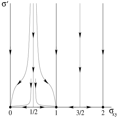
FIG. 2.: Large N renormalization group flow diagram for $\sigma^{\prime}=\sigma^{\prime}_{xx}/N$ and the “Hall conductance” $\sigma^{\prime}_{xy}=k(\nu)+\theta^{\prime}/2\pi$. The arrows indicate the direction toward the infrared.

$\bullet$Conductance fluctuations.    Rather than expanding $S^{\prime}_{bulk}$ in powers of $C[q]$ we next elaborate on the leading order result, valid for $0<\theta(\nu)<\pi$

$$S^{\prime}_{bulk}[q] = F(\theta)-\ln\int d\theta^{\prime}P(\theta^{\prime})e^{i\theta^{\prime}C[q]}.$$ (25)

$$P(\theta^{\prime}) = (1-\frac{<\theta^{\prime}>}{2\pi})\delta(\theta^{\prime})+\frac{<\theta^{\prime}>}{2\pi}\delta(\theta^{\prime}-2\pi).$$ (26)

Here, $P(\theta^{\prime})$ indicates that the quantity $\theta^{\prime}$ is actually distributed in an highly non-gaussian manner. The expectation $<\theta^{\prime}>$ is precisely the same as $\theta^{\prime}$ in Eq. (23). Notice that in the ‘quantum Hall phase’ $<\theta^{\prime}>$ vanishes exponentially in $L^{2}$, along with the higher order moments. At the transition, however, we have $<\theta^{\prime}>=\sqrt{<(\theta^{\prime}-<\theta^{\prime}>)^{2}>}=\pi$ which is large $N$ version of the broad mesoscopic conductance fluctuations that typically occur at the quantum Hall plateau transitions [11].

$\bullet$Twisted boundary conditions.    Following ’t Hooft’s idea we next employ Eq. (25) to compute the response of the bulk of the system to twisted boundary conditions [1]. For this purpose we evaluate $S^{\prime}_{bulk}$ with $C[q]=\frac{1}{2}$ relative to the result with integral topological charge

$$\Delta S^{\prime}_{bulk}=-\ln(1-<\theta^{\prime}>/\pi).$$ (27)

Notice that for $\theta(\nu)<\pi$ the response is exponentially small in the area of the system, $\Delta S^{\prime}_{bulk}\approx<\theta^{\prime}>/\pi\approx e^{-L^{2}/\xi^{2}(\nu)}$, as expected. However, as one approaches the transition, $\theta(\nu)=\theta^{\prime}=\pi$, the response diverges logarithmically. Hence, gapless bulk excitations must exist at $\theta(\nu)=\pi$. This is in spite of the fact the large $N$ system is insensitive to a change from periodic to anti-periodic boundary conditions. The research was supported in part by FOM and INTAS (Grant 99-1070).

REFERENCES

- [1] H. Levine, S. Libby and A.M.M. Pruisken, Phys. Rev. Lett. 51, 20 (1983)
- [2] A.M.M. Pruisken, Nucl. Phys. B285 719 (1987), B290 61 (1987).
- [3] A.M.M. Pruisken, Phys. Rev. Lett. 61, 1297 (1988)
- [4] H.P. Wei et al Phys. Rev. Lett. 61, 1294 (1988); for recent results see R.T.F. van Schaijk et al, Phys. Rev. Lett. 84,1567 (2000)
- [5] A.M.M. Pruisken, B. Škorić and M. Baranov, Phys. Rev. B60, 16838 (1999)
- [6] S. Coleman, Aspects of Symmetry (University Press, Cambridge) 1989
- [7] A. D’Adda, P. Di Vecchia and M. Luescher, Nucl. Phys. B 146, 63 (1978)
- [8] E. Witten, Nucl. Phys. B 149, 285 (1979)
- [9] I. Affleck, Nucl. Phys. B 162, 461 (1980); 171, 420 (1980)
- [10] A.M.M. Pruisken, M.A. Baranov, and M. Voropaev, e-print cond-mat/0101003.
- [11] M.H. Cohen and A.M.M. Pruisken, Phys. Rev. B49, 4593 (1994).