Adsorption hysteresis and capillary condensation in disordered porous solids: a density functional study.

Abstract

We present a theoretical study of capillary condensation of fluids adsorbed in mesoporous disordered media. Combining mean-field density functional theory with a coarse-grained description in terms of a lattice-gas model allows us to investigate both the out-of-equilibrium (hysteresis) and the equilibrium behavior. We show that the main features of capillary condensation in disordered solids result from the appearance of a complex free-energy landscape with a large number of metastable states. We detail the numerical procedures for finding these states, and the presence or absence of transitions in the thermodynamic limit is determined by careful finite-size studies.

I Introduction

Capillary condensation of a gas in a single, infinitely long pore of simple geometry (e.g., a slit) is a genuine first-order phase transition that corresponds to the shift of the bulk gas-liquid transition due to confinement and adsorption on the solid walls E1990 . The jump in the mean density of the confined fluid occurs at a vapor pressure smaller than the bulk saturation value $P_{sat}$ and disappears above a capillary critical temperature $T_{cc}$ that is lower than the bulk critical temperature $T_{c}$. As is usual with first-order phase transitions, the existence of local free-energy minima associated with the competing phases may result in hysteretic behavior as the control variable (here, the vapor pressure or, equivalently, the chemical potential) is swept upward and downward. In a mean-field description of the phase transition, the metastable portions of the gas and liquid branches exist only below $T_{cc}$, and the hysteresis loop is similar to that in the van der Waals equation of state of a subcritical bulk fluid.

This theoretical picture is, however, inadequate to describe the experimental situation of fluids adsorbed in mesoporous solids like porous glasses or silica gelsGGRS1999 . Indeed, these amorphous materials contain a highly interconnected, irregular, three-dimensional pore network, and one observes at low temperatures a steep increase of the adsorbed quantity at pressures below $P_{sat}$, but no sharp vertical jump that would be the undisputable signature of a first-order transition (a noticeable exception is the case of very dilute aerogelsWC1990 ; Z1996 ). There are also no density fluctuations on large length scales that would signal the onset of criticality. The main phenomenon is a hysteresis in the sorption isotherms between filling and draining, with a marked asymmetry between the adsorption and the desorption branches. The hysteresis loop shrinks in size as the temperature increases and eventually disappears above a certain temperature $T_{h}$ lower than $T_{c}$. There is also a whole hierarchy of subloops and scanning curves that are obtained by performing incomplete filling-draining cycles B1963 . Hysteresis loops are perfectly reproducible on the time-scale of usual adsorption experiments and are widely used for characterization of porous materials GS1982 , despite the fact that a satisfactory understanding of the physical mechanism is still missing. In particular, the question of whether hysteresis results solely from metastability in each pore or from the interconnectivity of the pore network is still a matter of debateBE1989 . Also, the connection between hysteresis (which is intrinsically an out-of-equilibrium phenomenon) and a possible underlying equilibrium transition remains largely unexplored. In fact, the absence of a sharp jump in the adsorption isotherm is usually taken as the indication that there is no thermodynamic phase transition in the porous material, the continuous filling being a consequence of the distribution of pore sizes and shapes. This can be justified in the framework of an independent-pore modelBE1989 ; E1967 ; LH2001 in which each pore is regarded as an isolated system, much like in the Preisach model of hysteresis in magnetic systemsP1935 . The global sorption isotherms are then obtained by performing an average over the distribution of pore sizes, an operation that smears out any discontinuous behavior of the elementary units. The independent-pore model, however, is a phenomenological description, with no microscopic justification, and it is in general impossible to characterize geometrically the independent domains.

In order to better understand these important issues, we have recently undertaken a detailed investigation of the equilibrium and out-of-equilibrium (hysteretic) properties of a lattice model introduced some years ago as a coarse-grained description of fluids in disordered solidsPRST1995 . Although simple, the model contains the essential physical ingredients that characterize such systems (confinement, randomness of the pore network, wettability of the solid surface) and it has a well-defined Hamiltonian, which allows to perform a statistical-mechanical calculation of the equilibrium properties. This contrasts with previous phenomenological descriptions of capillary condensation that use predefined kinetic rules for the evolution of the fluid configurations in the pore spaceM1982 . Like in most theoretical studies of capillary condensation (see, e.g., Ref.E1990 and references therein), our analysis is based upon mean-field density functional theory (i.e., local mean-field theory in the terminology of lattice models). As shown in preliminary reports on this workKRTV2001 ; KMRST2001 , our theoretical predictions qualitatively reproduce many aspects of the phenomenology of capillary condensation, in particular the asymmetry of the hysteresis loops, their temperature dependence, and the shape of the scanning curves. This demonstrates the relevance of the model and supports the hypothesis that thermal fluctuations, which are ignored in a mean-field treatment, play a minor role on the time scale of adsorption experiments (a feature confirmed by Monte-Carlo simulations performed on related modelsSM2001 ; WM2002 ). Our results suggest that the experimental observations mainly reflects the complexity of the underlying free-energy landscape at low temperatures. Indeed, quite similarly to disordered magnetic systems, such as spin-glasses or random-field spin models, that have been extensively studied in recent yearsN1997 , we find a large number of metastable states below a certain temperature. As one varies the external control parameter (here, the chemical potential), the system either follows a given local minimum of the free-energy surface or, when the local minimum looses its stability, jumps to another, nearby minimum. This results in a hysteretic behavior. It also causes a loss of thermodynamic consistency along the sorption isotherms, a feature that cannot be explained in the framework of the classical van der Waals picture of metastability where only two free-energy minima are present below $T_{c}$. As far as the equilibrium properties are concerned, we find that a genuine thermodynamic phase transition may occur when the perturbation induced by the solid is sufficiently small, which is at odds with the picture built upon the independent-pore model. Moreover, the existence of this underlying transition cannot be deduced from the behavior of the adsorption branch that may be either continous or discontinuous.

The goal of the present work is to give a general picture of capillary condensation in disordered mesoporous materials, to detail some of the mean-field density functional theory (DFT) calculations, and to report on new results. The paper is arranged as follows. In Section II we review the model and the theory, and we describe the numerical procedures used to find the solutions of the DFT equations. Section III presents the results for the hysteresis loops and the scanning curves. Section IV is devoted to a detailed analysis of the DFT equilibrium isotherms; a careful finite-size scaling study is performed to check on the presence or absence of a sharp transition in the infinite volume limit. We summarize our main findings in Section V.

II Model and theory

II.1 Model

We consider a three-dimensional lattice where each of the $N$ sites ($i=1,2,..N$) may be occupied by a fluid or a matrix particle, as described by the occupancy variables $\tau_{i}$ and $1-\eta_{i}$, respectively ($\tau_{i}=1$ if site $i$ is occupied by a fluid particle and $\tau_{i}=0$ if it is not, $\eta_{i}=0$ if site $i$ is occupied by a matrix particle and $\eta_{i}=1$ if it is not). Multiple occupancy of a site is forbidden and only nearest neighbor (n.n.) interactions are taken into account. The associated Hamiltonian isPRST1995 ; KRTP1998

$${\cal H}=-w_{ff}\sum_{<ij>}\tau_{i}\tau_{j}\eta_{i}\eta_{j}-w_{mf}\sum_{<ij>}[\tau_{i}\eta_{i}(1-\eta_{j})+\tau_{j}\eta_{j}(1-\eta_{i})]$$ (1)

where $w_{ff}>0$ and $w_{mf}$ denote the fluid-fluid and matrix-fluid interactions, respectively, and the sums run over distinct n.n. pairs. Fluid particles are in thermal equilibrium with an external reservoir that fixes their chemical potential $\mu$ and the temperature $T$, whereas matrix particles are distributed according to some given probability distribution function $P(\{\eta_{i}\})$. In the simplest version of the model that is considered in this work, the matrix particles are distributed randomly on the lattice with the canonical constraint that $\sum_{i}\eta_{i}=(1-\rho_{m})N$, where $\rho_{m}$ is the matrix density.

This is clearly a coarse-grained description that leaves aside most of the microscopic details of an actual solid-fluid system. However, experiments show that fluids in disordered media share some generic qualitative properties. These latter can then be captured by a simple model, with the great advantage that the model is amenable to detailed numerical investigations. The model has only two parameters that can be tuned independently: $1-\rho_{m}$, the porosity of the matrix (here, dilution plays the role of confinement), and $y=w_{mf}/w_{ff}$, the interaction ratio that controls the wetting properties of the solid-fluid interface. One can easily improve the description, for instance by using a distribution of the matrix particles that is more faithfull to the microstructure of a real solidSM2001 ; WSM2001 ; DKRT2002 .

By transforming the above lattice-gas Hamiltonian to its equivalent spin-$\frac{1}{2}$ Ising formKRTP1998 , one finds that the value $y=1/2$ plays a special role. Indeed, at fixed $\rho_{m}$, there is a symmetry $y\leftrightarrow 1-y$ expressed by

$$\rho_{i}(y,\mu,T)+\rho_{i}(1-y,-\mu-cw_{ff},T)=\eta_{i}\,$$ (2)

where $c$ is the coordination number of the lattice and $\rho_{i}=<\tau_{i}\eta_{i}>$ is the average fluid density at site $i$ for a given realisation of the random matrix defined by the set $\{\eta_{i}\}$. (Throughout the paper we denote by $<..>$ the thermal average for a given matrix sample and by $[..]$ the ensemble average over the different matrix samples.) This property (that is special to the lattice-gas description) allows us to restrict the study to $y\geq 1/2$ and to attractive solid-fluid interactions only. It is important to note that $y=1/2$ is the only case where the hole-particle symmetry of the bulk lattice gas is preserved. The Hamiltonian described by Eq. (1) is then equivalent to that of the site-diluted Ising model, a model for disordered magnets whose properties are well-documentedS1983 . In particular, this mapping tells us immediately that the system undergoes a liquid-vapor phase separation at low temperature when the porosity is large enough. Specifically, the critical temperature $T_{cc}(\rho_{m},y=1/2)$ decreases monotonically from $T_{c}$ to $0$ as $\rho_{m}$ varies from $0$ up to $1-p_{c}$, where $p_{c}$ is the site-percolation threshold of the lattice. Moreover, because of the hole-particle symmetry, the transition takes place at the same chemical potential as the bulk liquid-gas transition, $\mu=\mu_{sat}=-cw_{ff}/2$.

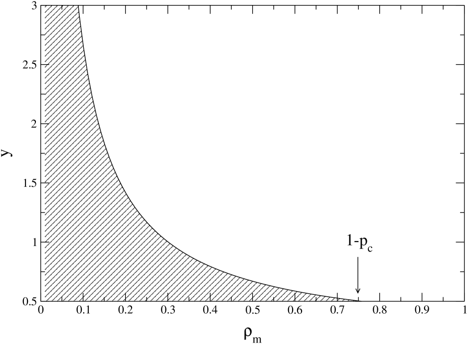
Figure 1: Putative equilibrium phase diagram of the model in the $\rho_{m}-y$ plane for $y\geq 1/2$. A genuine capillary condensation occurs for $T<T_{cc}(\rho_{m},y)$ in the hatched region with $T_{cc}(\rho_{m},y)=0$ at the boundary. For $\rho_{m}>1-p_{c}$, there is no phase transition because the void space ceases to percolate.

The physical behavior for $y\neq 1/2$ is more complicated, but more relevant to real adsorption experiments; then, random fields come into play in addition to dilution, which breaks the up-down (or hole-particle) symmetry of the modelKRTP1998 ; SP1992 . These random fields are spatially correlated (at a local scale, though) and can take $c+1$ distinct values at a fluid site $i$, depending on the number $n_{i}$ of n.n sites that are occupied by a matrix particle ($0\leq n_{i}\leq c$). For a purely random matrix, one has $P(n_{i})=\binom{c}{n_{i}}\rho_{m}^{n_{i}}(1-\rho_{m})^{c-n_{i}}$ which leads to a binomial distribution of the fieldsMSCCCB1991 . On general grounds, one expects that the presence of random fields has dramatic consequences for the out-of-equilibrium properties of the model (see, e.g., Ref.FGK1988 ). According to the original argument of Imry and MaIM1975 based on the energy balance for domain formation, this sort of randomness should not forbid the system from undergoing a sharp thermodynamic transition at low temperature in three dimensions; but it should strongly alter the critical propertiesN1997 . Specifically, as will be illustrated by the calculations of section IV, we expect that there is a nonzero critical temperature $T_{cc}(\rho_{m},y)$ when the effective strength of the disorder is weak, i.e., when $\rho_{m}$ is smaller than a certain value $\rho_{m}^{max}(y)$ (or $y$ smaller than $y_{max}(\rho_{m}))$. Moreover, since the random fields have a mean that is strictly positive for $y>1/2$, the jump in the fluid density for $T<T_{cc}(\rho_{m},y)$ occurs at a chemical potentiel that is lower than $\mu_{sat}$: this first-order phase transition is thus a genuine equilibrium capillary condensation. This leads to the putative phase diagram shown in Fig. 1 where the boundary between the two regions corresponds to $T_{cc}(\rho_{m},y_{max}(\rho_{m}))=0$. (In fact, as will be discussed below, the behavior of finite matrix samples is rather complicated and one cannot discard the possible existence of two or more phase transitions occuring at different chemical potentials, as found in a previous workKRTP1998 ).

II.2 Mean-field density functional theory

There are essentially two different approaches for studying the statistical properties of fluids or magnets in the presence of quenched disorder. The first one is the replica method in which only quantities that are averaged over the disorder can be calculated. This is the method that we have used in our preceding studies of fluids in porous solidsPRST1995 ; KRTP1998 ; KMRT1997 where we have derived formal equations for the fluid-fluid and matrix-fluid average (hence, translationally invariant) pair correlation functions. In principle, the solution of these equations, supplemented by some appropriate closure approximations, yields the equilibrium properties of the model in the thermodynamic limit. However, standard approximations of liquid-state theory may run into difficulties in the presence of a large number of metastable states (as is the case here). Moreover, the physical content of this formulation is not very transparent, especially if replica symmetry breaking occurs. The second method consists in first calculating the properties of a single finite sample and averaging the results over the disorder at a later stage of the calculation, as was done by Thouless-Anderson-Palmer in their study of the infinite-range Ising spin-glass modelTAP1977 . This is the approach that we choose in the present work because it allows us to investigate the free-energy landscape for a given disorder realization and to understand its relation to the hysteretic behavior of the model. The main inconvenience of working with finite samples is that a careful finite-size scaling study is needed in order to conclude on the existence of sharp phase transitions in the infinite-volume limit. This usually requires a significant amount of numerical analysis.

We thus consider a finite lattice of linear size $L$ and, in order to simplify the numerical work and to minimize surface effects, we use periodic boundary conditions in all directions. The adsorbed fluid is then statistically homogeneous, with a mean density $\rho_{f}=(1/N)\sum_{i}\rho_{i}=[<\tau_{i}\eta_{i}>]$ in the limit of a large system. As discussed elsewhereSM2002 ; KRT2002 , choosing periodic boundary conditions is not completely benign: it may alter dramatically the nature of the desorption process, but has no consequences for the equilibrium properties nor, for the problem at hand, for the adsorption process.

For a given realization of the random matrix, the DFT starts with the expression of the grand-potential functional of the fluid-density field (on a lattice, the functional is actually a function of the $\{\rho_{i}\}$’s)KRTV2001 ; KMRST2001 :

$$\Omega(\{\rho_{i}\}) = k_{B}T\sum_{i}[\rho_{i}\ln\rho_{i}+(\eta_{i}-\rho_{i})\ln(\eta_{i}-\rho_{i})]$$ (3)

$$- w_{ff}\sum_{<ij>}\rho_{i}\rho_{j}-w_{mf}\sum_{<ij>}[\rho_{i}(1-\eta_{j})+\rho_{j}(1-\eta_{i})]-\mu\sum_{i}\rho_{i}\ ,$$

an expression that is obtained as usual in a mean-field approximation by neglecting correlations between the thermal fluctuations of the instantaneous fluid densities, $\tau_{i}\eta_{i}-<\tau_{i}\eta_{i}>$. It should be stressed, however, that the present approach fully accounts for the disorder-induced fluctuations, fluctuations that are expected to be the dominant ones in systems with random fieldsN1997 . It also preserves all geometric constraints and, as a result, properly describes the site percolation threshold.

Minimization with respect to the $\{\rho_{i}\}$’s leads to the following equations:

$$\rho_{i}=\eta_{i}[1+e^{-\beta v^{eff}_{i}}]^{-1}$$ (4a)

where $$\beta=1/(k_{B}T) v^{eff}_{i} i$$ and is the effective potential at site ,

$$v^{eff}_{i}=\mu+w_{ff}\sum_{j/i}[\rho_{j}+y(1-\eta_{j})]\ ,$$ (4b)

where the sum runs over the $c$ nearest neighbors of site $i$. It is easy to see that these $N$ coupled non-linear equations are invariant in the change $\mu\leftrightarrow-\mu-cw_{ff},y\leftrightarrow 1-y,\rho_{i}\leftrightarrow\eta_{i}-\rho_{i}$, which shows that the mean-field DFT is faithfull to the symmetry property expressed by Eq. (2). There are in general several solutions to Eqs. (4), that can be maxima, saddle-points, as well as minima of the grand-potential functional. In what follows, we focus only on the metastable states, i. e., on the minima. We label these latter by the superscript $\alpha$. The grand potential for the solution $\{\rho_{i}^{\alpha}\}$ is then given byKRTV2001

$$\Omega^{\alpha}=k_{B}T\sum_{i}\eta_{i}\ln(1-\frac{\rho_{i}^{\alpha}}{\eta_{i}})+w_{ff}\sum_{<ij>}\rho_{i}^{\alpha}\rho_{j}^{\alpha}\ .$$ (5)

The adsorbed fluid is in equilibrium with a bulk fluid whose uniform density $\rho_{f}^{bulk}$ satisfies the standard mean field equation of state of a n.n. lattice gas, which yields a critical point located at $k_{B}T_{c}/w_{ff}=c/4$ and $\rho_{f}^{c}=1/2$.

For a given matrix realisation and a given temperature, Eqs. (4) were solved by the simplest iterative method: an initial set of local densities, $\{\rho_{i}^{(0)}\}$, was used to calculate a set of effective local potentials, $\{v^{eff(0)}_{i}\}$, from which a new set of densities was generated, and so on, until a fixed point of the iterative procedure was obtained. The main interest of such an algorithm is that it automatically discards solutions of Eqs. (4) that are not minima of the grand potentialLBL1983 .

Two types of numerical calculations were performed. First, to mimic the protocol of sorption experiments, we progressively increased (respectively, decreased) the chemical potential from a large negative (respectively, from the bulk saturation) value, using at each subsequent $\mu$ the converged values of the $\rho_{i}$’s at the previous chemical potential to start the iteration (the elementary step was $\Delta\mu/w_{ff}=10^{-2}$ or $10^{-3}$). At each $\mu$, convergence was assumed when $(1/N)\sum_{i}(\rho_{i}^{(n+1)}-\rho_{i}^{(n)})^{2}<10^{-8}$, where the superscript $(n)$ denotes the nth iteration. More complicated chemical potential histories were also considered to describe the adsorption and desorption scanning curves or the inner hysteresis loops. Secondly, to search for other solutions of Eqs. (4), we generated at each $\mu$ a certain number of initial configurations (typically, $10^{2}$) corresponding to uniform fillings of the lattice with different overall fluid densities (i.e. $\rho_{i}^{(0)}=\rho_{f}^{0}$). Our objective was not an exhaustive enumeration of all solutions. Indeed, a more systematic search would require the use of non-uniform seed configurations such as random or chequerboard configurationsLMP1995 ; MPP2000 . However, our set of initial configurations was in general sufficient to obtain a good approximation of the equilibrium solution (i.e., that giving the lowest value of $\Omega$) in the range of temperatures explored in the present work. This search required a rather stringent convergence criterion: the iteration algorithm was stopped when $(1/N)\sum_{i}(\rho_{i}^{(n+1)}-\rho_{i}^{(n)})^{2}<10^{-14}$, and two solutions $\{\rho_{i}^{\alpha}\}$ and $\{\rho_{i}^{\beta}\}$ were considered as different whenever $\sum_{i}(\rho_{i}^{\alpha}-\rho_{i}^{\beta})^{2}>10^{-6}$. (We indeed observed, as in Ref.LMP1995 , that different initial conditions could yield the same final configuration.)

The above mean-field DFT (or local mean-field) equations have an interesting property that is worth pointing out. Suppose that for a given realization $\{\eta_{i}\}$, two different sets $\alpha$ and $\beta$ of fluid densities satisfy the condition $\rho_{i}^{\alpha}\leq\rho_{i}^{\beta}$ for each site in the system (this is of course a very special ordering: most fluid configurations do not have such a relationship). Then, because of the convexity of the exponential function, the densities on the left-hand side of Eq. (4a) satisfy the same ordering. This ordering is thus automatically preserved by the iteration algorithm. In particular, any solution of Eqs. (4) yields a mean fluid density $\rho_{f}$ that is larger (respectively, lower) than the density obtained by starting the iteration procedure from an initially empty (respectively, filled) lattice. This defines two extremal curves that coincide with the adsorption and desorption isotherms. For the same reason, the algorithm satisfies a “no-passing” ruleM1992 which implies a so-called return-point memory property: when the chemical potential is adiabatically (i.e., very slowly) swept upward, downward and then upward again (or conversely) so as to come back to its original value, the system returns to exactly the same configuration of the $\rho_{i}$’s (and thus to the same mean density $\rho_{f}$). This is fully equivalent to the return-point memory property observed in ferromagnetic systems, and the demonstration of the “no-passing” rule is similar to that given by Sethna et al.S1993 for the athermal dynamical response of the random-field Ising model to an external field. Clearly, using an iterative numerical mean-field scheme is analogous to having a zero-temperature dynamics: the system only evolves under the influence of the external control parameter (magnetic field or chemical potential), and there is no possible equilibration mechanism via thermally activated processes that would take the system from one metastable state to another. In the absence of a satisfactory theoretical treatment of these effects, it is the comparison to computer simulations or to experiments that can tell us whether the qualitative picture emerging from this calculation is modified or not by thermal fluctuationsWM2002 .

For various system sizes, Eqs. (4) were solved for many matrix samples, and the results were then averaged over this set of matrix realizations. The number of samples depended on the lattice size and on the property studied. To obtain the hysteresis loops and the scanning curves, it was sufficient to use a small number of realizations. Indeed, the determination of the adsorption/desorption isotherms did not require a large amount of computational effort so that rather large samples (with typically $L=48$) could be usedrem . On the other hand, the search for the equilibrium isotherms was much more demanding, and we had to consider smaller systems ($L=8,10,12,$ and $16$) to perform the finite-size study described in Sec. IV. The model has a good self-averaging behavior far from criticality and good statistics could be reached with a few hundreds samples.

All the results presented here are obtained for a bcc lattice ($N=2L^{3},c=8$). The present model has a rich behavior and it would be interesting to perform a systematic study of its properties as a function of $\rho_{m},y$ and $T$. This task, unfortunately, would require a considerable amount of computational work. We are thus limited to select a few points in the parameter space, which we think represent typical situations. We consider a single value of the matrix density, $\rho_{m}=0.25$, which is just above the site percolation threshold of the lattice, $p_{c}=0.243$SA1994 , and a single temperature, $T^{*}=k_{B}T/w_{ff}=0.8$, which is well below the mean-field critical temperature of the bulk fluid, $T_{c}^{*}=2$. We defer the study of the influence of the temperature and the porosity on the behavior of the adsorbed fluid to a future work in which the matrix sites will be distributed over the lattice in a non-random and more realistic fashionDKRT2002 .

III Hysteresis loops and scanning curves

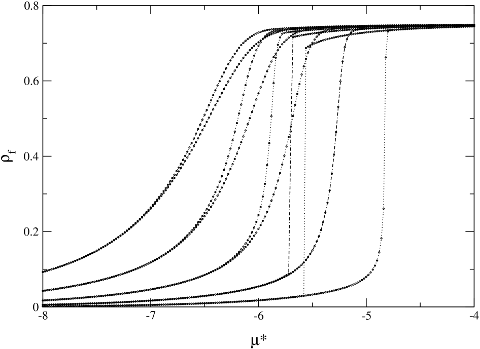
Figure 2: DFT prediction for the sorption isotherms, $\rho_{f}$ versus $\mu*=\mu/w_{ff}$, for $T^{*}=0.8$ and $\rho_{m}=0.25$. From left to right: $y=2$, $1.75$, $1.50$, $1.25$, and $1$. The results have been averaged over $10$ matrix samples of linear size $L=48$. Recall that at complete filling, $\rho_{f}=1-\rho_{m}=0.75$.

We first consider the hysteretic, out-of-equilibrium behavior of the system which can be described within the mean-field DFT by using the first protocol described above. Representative adsorption and desorption isotherms are shown in Fig. 2 where the mean fluid density $\rho_{f}$ is plotted versus the reduced chemical potential $\mu^{*}=\mu/w_{ff}$ for several values of the interaction ratio $y$. When $y$ increases, i. e., when the matrix-fluid interaction gets stronger, more fluid can be reversibly adsorbed in the vicinity of the matrix particles, and the hysteresis loop shrinks and occurs further away from the bulk saturation value, $\mu^{*}=-4$.

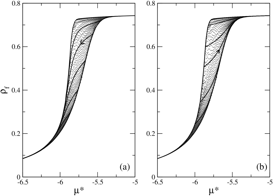
Figure 3: DFT predictions for the desorption (a) and adsorption (b) scanning curves for $y=1.5$ in a matrix of linear size $L=48$. Also shown are the many metastable states obtained by solving Eqs. (4) according to the second protocol described in the text.

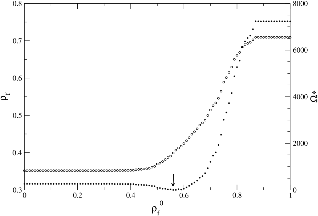
Figure 8: Average fluid density $\rho_{f}$ (circles) and reduced grand-potential $\Omega^{*}$ (stars) as functions of the initial seed density $\rho_{f}^{0}$ for $y=1.5$ and $\mu^{*}=-5.80$ ($L=48$). Here $\Omega$ is measured with respect to its minimum value, $\Omega^{eq}$, obtained for $\rho_{f}^{0}=0.56$ (arrow).

Scanning curves obtained by performing incomplete filling of the matrix and then decreasing the chemical potential to drain the adsorbed fluid (desorption scanning curves) or by the reverse procedure of incomplete draining before filling (adsorption scanning curves) are illustrated in Figs. 3a and 3b for $y=1.5$. As seen by comparing the two figures, the shape of the curves is markedly different on desorption and adsorption. The theoretical predictions are strikingly similar to those measured by BrownB1963 for Xe in Vycor, a porous glass (see, e.g., Fig. 8 in Ref.BE1989 ), which supports our claim that the present coarse-grained model contains the important physical ingredients to describe adsorption in disordered porous media. As stressed by Ball and EvansBE1989 , the shape of the predicted scanning curves is indeed a rather stringent test for the validity of any proposed model. In particular, the independent-pore model (or Preisach modelP1935 in the context of magnetic systems) does not properly account for the observed curves.

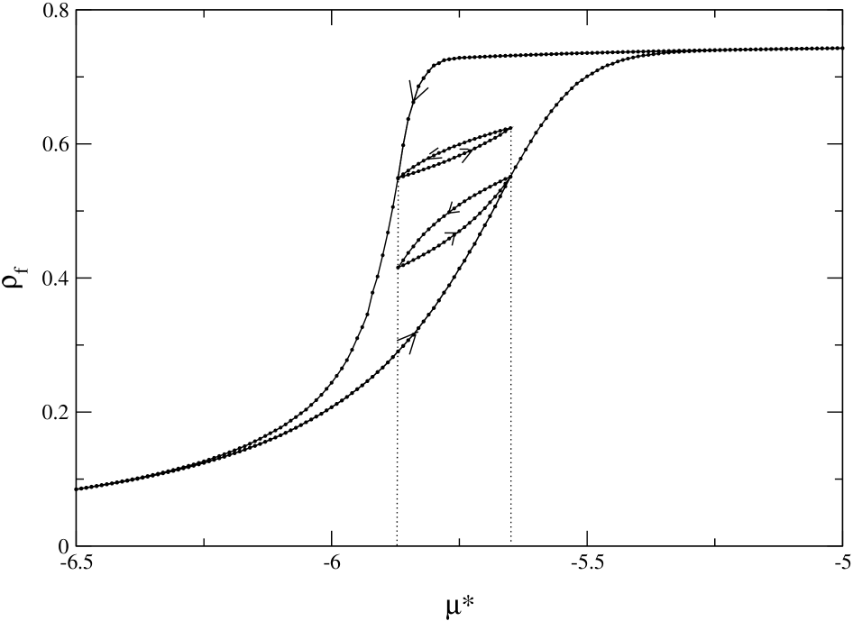
Figure 4: DFT predictions for the global hysteresis loop and two representative subloops for $y=1.5$. The arrows denote the different filling-draining cycles. The results have been averaged over 10 matrix samples of linear size $L=48$.

Connectivity of the pore network shows up distinctly when considering hysteresis subloops obtained by performing more complicated cycles of the chemical potential than those considered so far. This is illustrated in Fig. 4. The two subloops shown in the figure display two characteristic features: first, the property of return-point memory already discussed and also satisfied by the independent-pore model; and second, the lack of congruence, which means that the two subloops, even though they open and close at the same chemical potentials, cannot be superimposed on top of each other by a mere translation along the vertical axis. Since, irrespective of its detailed implementation, the independent-pore model predicts exact congruence, a lack of congruence is a clear-cut signature of the connectivity of the pore spaceWH2000 .

The physical reason for the presence of hysteresis loops, scanning curves, and various subloops is the existence of many metastable states in which the system gets trapped, at least on the time scale of the experiment. If thermally activated processes that could allow for untrapping from these metastable states are characterized by time scales longer than the experimental time scale, the system can only evolve under the influence of an external driving force, i.e., a change in the chemical potential. This is precisely the situation described by the mean-field DFT approach. The grand-potential free-energy hypersurface (or, to use a more pictorial term, “landscape”) defined by Eq. (3), $\Omega$ as a function of the $\{\rho_{i}\}$’s, evolves with $\mu$: a given minimum can be continuously deformed and at some point looses its stability and disappears. Hysteresis loops, scanning curves, and other hysteresis subloops (as illustrated in Fig. 4) correspond to various paths among minima of the grand-potential landscape. To make this more visual, we have also plotted in Figs. 3a and b the minima obtained from the DFT by following the second protocal described in section II B.

The above landscape picture allows one to understand another puzzling feature associated with hysteresis. Based on the standard van der Waals description of metastability, it is often assumed that thermodynamics can still be used to describe the behavior of the fluid along the adsorption and desorption isotherms, even in the region of hysteresis. However, as illustrated in Figs. 5a and b, again for $y=1.5$, this assumption may fail in disordered porous materials. We compare in these figures the mean fluid density $\rho_{f}$ directly obtained from the solution of Eqs. (4) with that obtained from the Gibbs adsorption relation, $\rho_{f}=-\left.\partial(\Omega/N)/\partial\mu\right|_{T}$, in which the fluid grand potential is computed from Eq. (5) and the derivative is numerically calculated with a step $\Delta\mu^{*}=0.01$. There is a clear violation of the thermodynamic consitency along both the adsorption and the desorption branches of the hysteresis. This can be rationalized by recalling that the system jumps occasionnally from one local minimum of the grand potential to another. Correspondingly, there are jumps in $\rho_{f}$ and $\Omega$. These jumps may be extremely small (as indicated by the smooth curves obtained for the adsorption and desorption isotherms), but the system then looses thermodynamic consistency between $\rho_{f}$ and the change in $\Omega$. This point will be further discussed in the next section on equilibrium properties.

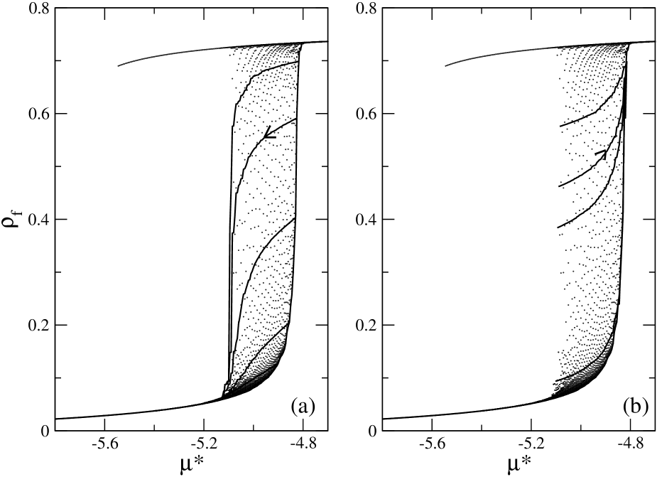
Figure 6: Same as Fig. 3 for $y=1$

All the above results were obtained for $y=1.5$. Qualitatively similar behavior is obtained for other values of the interaction ratio, e.g., for $y=1$. Figs. 6a and b display the hysteresis loop, several desorption and adsorption scanning curves, as well as metastable states obtained by solving Eqs. (4) according to the second protocol of section II.B. The main difference with the curves shown in Figs. 3a and b for $y=1.5$ is the presence of a line of metastable liquid states on the desorption branch that considerably widens the hysteresis loop. This line, which is accompanied by no other metastable states in a whole range of chemical potentials except the gas-like states on the adsorption branch, is actually an artefact of the periodic boundary conditions used in the present calculation. As shown elsewhereSM2002 ; KRT2002 , these liquid-like states become unstable as soon as one introduces a physical interface between the matrix and the external reservoir.

IV Equilibrium isotherms

As pointed out in the preliminary reports on this workKRTV2001 ; KMRST2001 , the existence of a complex free energy landscape changes dramatically the description of capillary condensation built upon the independent pore model and the standard van der Waals picture of phase transitions. In particular, determining the equilibrium state that yields the lowest value ot the grand potential becomes a non-trivial task, as explained in this section. For simplicity, we again restrict our study to the cases $y=1.5$ and $y=1$, two values of the interaction ratio that illustrate the system behavior in the two regions of Fig. 1 corresponding to the strong- and low-disorder regimes, respectively.

IV.1 The strong-disorder regime

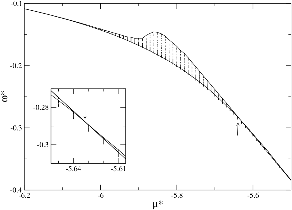
Figure 7: Reduced grand-potential density, $\omega^{*}=\Omega/(Nw_{ff})$, associated with the solutions of the mean-field equations for $y=1.5$ ($L=48$). The arrow indicates the crossing of the adsorption and desorption branches and the inset shows a zoom up of this region.

To each solution $\{\rho_{i}^{\alpha}\}$ of the mean-field equations, obtained by the search procedure explained in section II.B, corresponds a local minimum $\Omega^{\alpha}$ of the grand potential given by Eq. (5). The result, of course, is sample-dependent. Fig. 7 shows the reduced grand-potential densities $\omega^{*}=\Omega/(Nw_{ff})$ corresponding to the metastable solutions found for $y=1.5$ in a matrix of linear size $L=48$ (this is the same sample as in Fig. 3). Two comments are in order. First, the curves for the adsorption and desorption branches, $\Omega^{ads}(\mu)$ and $\Omega^{des}(\mu)$, cross each other at some value of the chemical potential, as indicated by the arrow in the figure (see inset). Therefore, by only considering the adsorption and desorption isotherms, one would predict the occurence of a first-order phase transition. (By naively integrating the Gibbs adsorption relation along the adsorption branch from $\mu=-\infty$ to a sufficiently large value, say $\mu=-4.5$, and along the desorption branch from $\mu=-4.5$ to $\mu=-\infty$ (see, e.g., Ref.STC1999 ), one would predict a crossing at another value of $\mu$; but this procedure cannot be used, as explained previously.) Secondly, a close inspection of the results in the region of hysteresis shows that the states that yield the absolute minimum of $\Omega$ do not belong to the adsorption or desorption branches (as can be seen in the inset of Fig. 7). This means that the true equilibrium isotherm is somewhere in between. This is illustrated in Fig. 8 where we plot the reduced grand potential $\Omega^{*}=\Omega/w_{ff}$ versus $\rho_{f}^{0}$, the uniform seed density used to start the iteration procedure at constant chemical potential (second protocal described in section II B). In this case, the lowest value of the grand potential, $\Omega^{eq}$, is obtained for $\rho_{f}^{0}=0.56$ and the associated value of the average fluid density is $\rho_{f}^{eq}=0.399$, whereas one has $\rho_{f}=0.352$ and $\rho_{f}=0.709$ on the adsorption and desorption branches, respectively. (Note that there are no other solutions than the extremal ones when $\rho_{f}^{0}<0.34$ and $\rho_{f}^{0}>0.86$.)

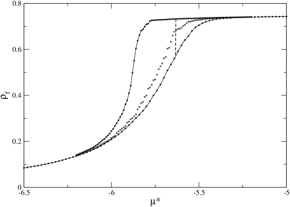
Figure 9: Hysteresis loop and equilibrium isotherm for $y=1.5$ ($L=48$). The dashed line indicates the first-order transition predicted by considering only the adsorption and desorption isotherms.

The same study, performed for each value of $\mu$, yields the equilibrium isotherm shown in Fig. 9. The curve is not smooth (there is a series of small jumps), but it is quite different from the pseudo-van der Waals, discontinuous isotherm constructed from the adsorption and desorption branches.

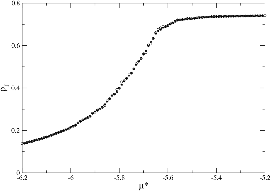
Figure 10: Check of thermodynamic consistency along the equilibrium isotherm for $y=1.5$ ($L=48$). Circles: average fluid density obtained from the solution of Eqs. (4). Stars: quantity obtained by differentiating the corresponding grand-potential.

Since our search of local minima is not exhaustive, it is important to check that we still get a good approximation of the true equilibrium isotherm. For instance, for some matrix realizations the calculated isotherm is not a monotonously increasing function of $\mu$ (i.e., $\partial\rho_{f}^{eq}/\partial\mu<0$), even when using a very small mesh size for $\rho_{f}^{0}$ : this implies that the equilibrium state cannot be found just with uniform seed configurations, and these samples were discarded. As a general rule, we find that the Gibbs adsorption equation, $\rho_{f}=-\left.\partial\omega/\partial\mu\right|_{T}$ is very well satisfied along the isotherm calculated from the locus of the lowest grand potential values, as shown in Fig. 10. This is in contrast with the behavior observed along the adsorption and desorption branches (see preceding section); contrary to what occurs along these latter, $\Omega^{eq}$ is a continuous function of $\mu$ even for finite-size samplesRem . This property of thermodynamic consistency that must be satisfied by the system at equilibrium can thus be used to control the success (or the failure) of the seed strategy for searching for the equilibrium state.

For some values of the chemical potential, we have also investigated how $\Delta\Omega$, the gap in grand potential between the two lowest minima, varies with the system size. These calculations, unfortunately, are computationally very demanding, and our results are too limited to conclude that $\Delta\Omega$ is an extensive quantity (i.e., of order $N$). We believe that this is an important issue that deserves a careful investigation in the near future: it is indeed possible that the system enters a “glassy phase” in some region of the parameter space, with several local minima contributing to the equilibrium properties in the thermodynamic limit (then $\Delta\Omega=O(1)$), as is the case for the RFIM near criticalityLMP1995 (this would correspond to a replica-symmetry breaking mechanism in the replica method). A convenient and intuitive way of taking into account this possibility is to consider a grand partition function that is a sum over all the solutions of the mean-field equations weighted by their associated Boltzmann factorDY1983 , i.e., $\Omega=-(1/\beta)\ln(\sum_{\alpha}e^{-\beta\Omega^{\alpha}})$. For all the sytems studied here (and $L$ sufficiently large) we have found that the isotherms calculated from this weighted mean-field approach are not significantly different from those obtained by only considering the solution with the lowest grand potential.

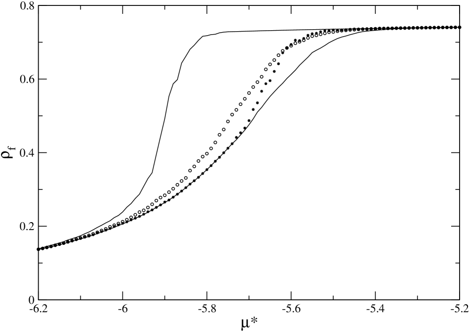
Figure 11: Hysteresis loop, equilibrium isotherm (circles) and pseudo-van der Waals isotherm (stars) for $y=1.5$ in a matrix of linear size $L=16$ . An average over $50$ matrix realizations has been performed.

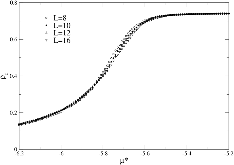
Figure 12: Equilibrium isotherms for $y=1.5$ and different system sizes. An average over $50$ $(L=16)$ to $400$ $(L=8)$ matrix realizations has been performed.

Finally, the isotherms obtained by averaging over many different matrix realizations are shown in Figs. 11 and 12. As usual, the averaging process smears out all the discontinuities present in the isotherms of the individual samples. Both the averaged equilibrium isotherm, $[\rho_{f}^{eq}(\mu)]$, and the curve obtained by averaging the pseudo-van der Waals isotherms obtained from the adsorption and desorption branches in each sample are smooth. (Note that this latter is different from the isotherm that would be obtained from looking at the crossing of the two averaged curves $[\Omega^{ads}(\mu)]$ and $[\Omega^{des}(\mu)]$: this again would lead to a discontinuity.) As can be seen in Fig. 11, the two curves are quite distinct, which stresses again the failure of the standard van der Waals picture. The equilibrium isotherm depends on the system size but this dependence is weak, as shown in Fig. 12. Moreover, the maximum value of $\partial[\rho_{f}^{eq}(\mu)]/\partial\mu$ stays almost constant (or even slightly decreases) as $L$ increases. We thus conclude that there is no transition at equilibrium in the infinite system.

IV.2 The weak-disorder regime

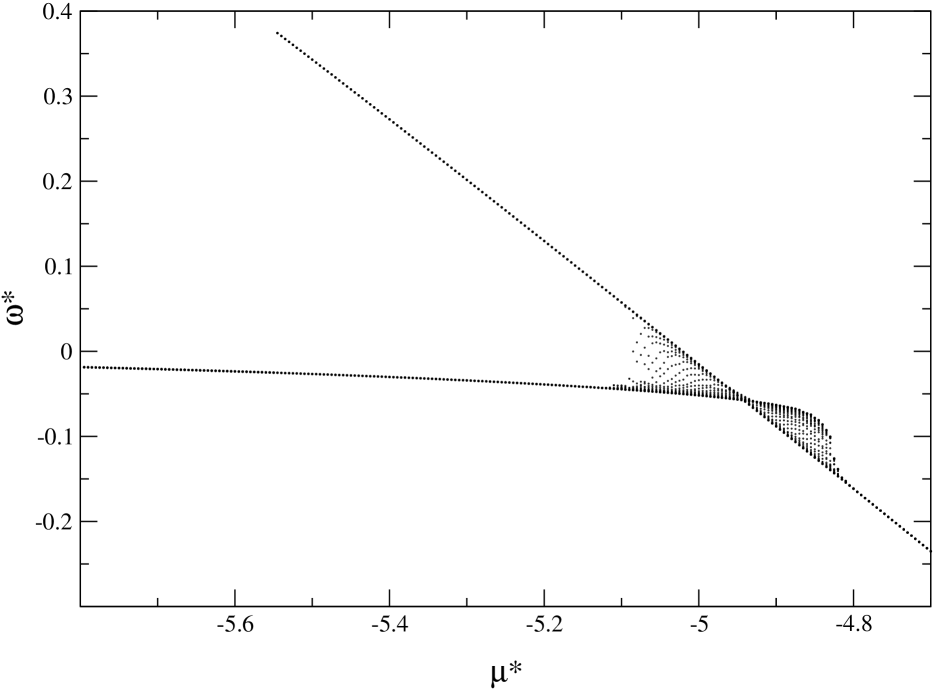
Figure 13: Reduced grand-potential density associated with the solutions of the mean-field equations for $y=1$ ($L=48$).

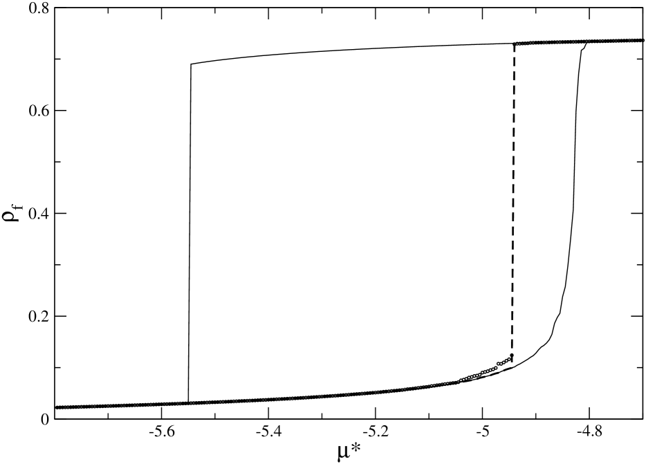
Figure 14: Hysteresis loop and equilibrium isotherm for $y=1$ ($L=48$). The dashed line indicates the first-order transition predicted by considering only the adsorption and desorption isotherms.

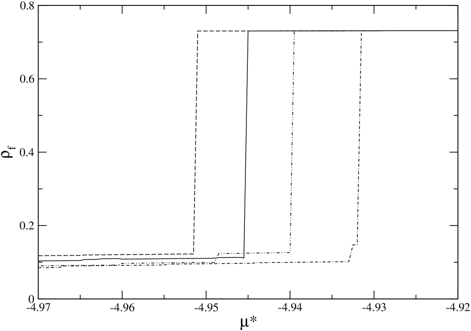
Figure 15: Equilibrium isotherms for $y=1$ and 4 matrix realizations of linear size $L=16$.

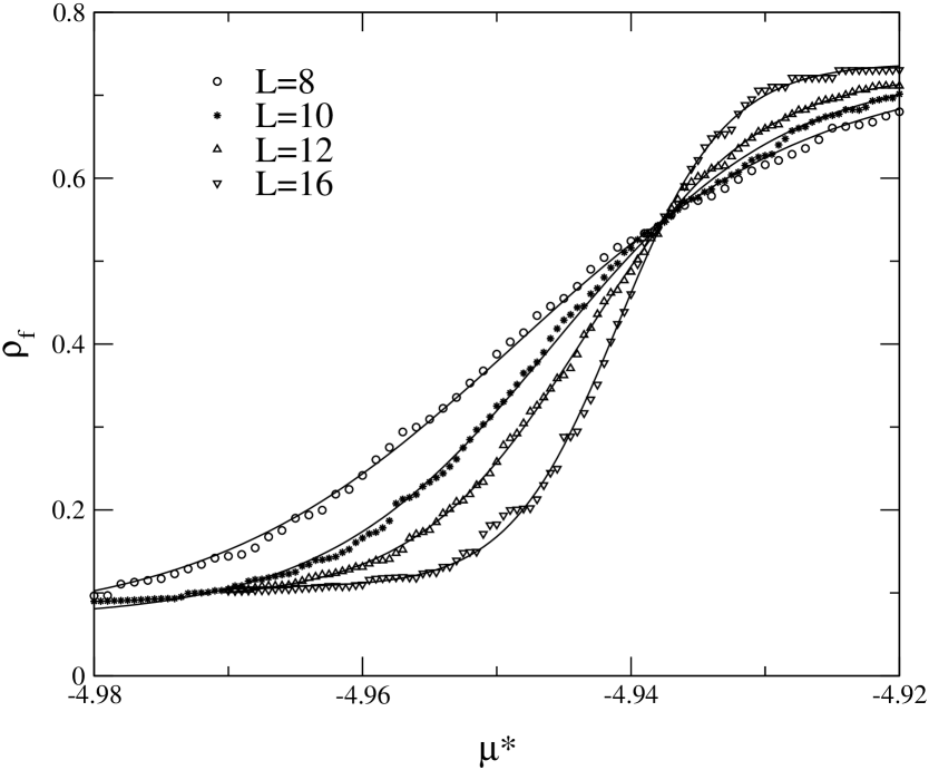
Figure 16: Equilibrium isotherms for $y=1$ and different system sizes. An average over $125$ $(L=16)$ to $400$ $(L=8)$ matrix realizations has been performed. The solid lines indicate the fit discussed in the text.

The grand-potential minima for $y=1$ and a matrix of size $L=48$ are presented in Fig. 13 (this is the same sample as in Fig. 6). As could be expected from the shape of the hysteresis loop, the presence of artificial liquid-like metastable states along the desorption isotherm results in a curve $\Omega^{des}(\mu)$ that is isolated from the other states and that ends abruptly. We have previously pointed out that this artefact is due to using periodic boundary conditions. But the main difference with the case $y=1.5$ concerns the states that yield the absolute minimum of the grand potential. They are indeed very close to the adsorption branch when $\Omega^{ads}<\Omega^{des}$ and to the desorption branch when $\Omega^{des}<\Omega^{ads}$. Accordingly, as shown in Fig. 14, one observes a large jump in the equilibrium isotherm at a chemical potential $\mu_{t}$ that is very close to the one at which $\Omega^{ads}=\Omega^{des}$. Since a similar jump in $\rho_{f}^{eq}$ is present in all matrix realizations, one may ask whether there exits a genuine first-order transition in the thermodynamic limit. To answer this question, one needs to perform a finite-size scaling analysis of the average equilibrium isotherm. In the present case, this study is somewhat complicated by the fact that the large jump is sometimes accompanied by several smaller discontinuities, as is the case for two of the isotherms shown in Fig. 15. This leads to an average isotherm that has a rather complex shape, as illustrated by the lower part of the $L=16$ curve in Fig. 16 showing the average equilibrium isotherms for various system sizes (we recall that this study is limited to rather small systems because of the considerable computational effort required by the search of the equilibrium states when $N$ is large). Although the appearance of several discontinuities may be a finite-volume artefact, the possible existence of two or more capillary transitions at different chemical potentials in the thermodynamic limit has been considered in a previous work using the replica formalismKRTP1998 . To investigate this question a separate analysis of the different parts of the isotherms is required, and we defer this delicate study to a future work.

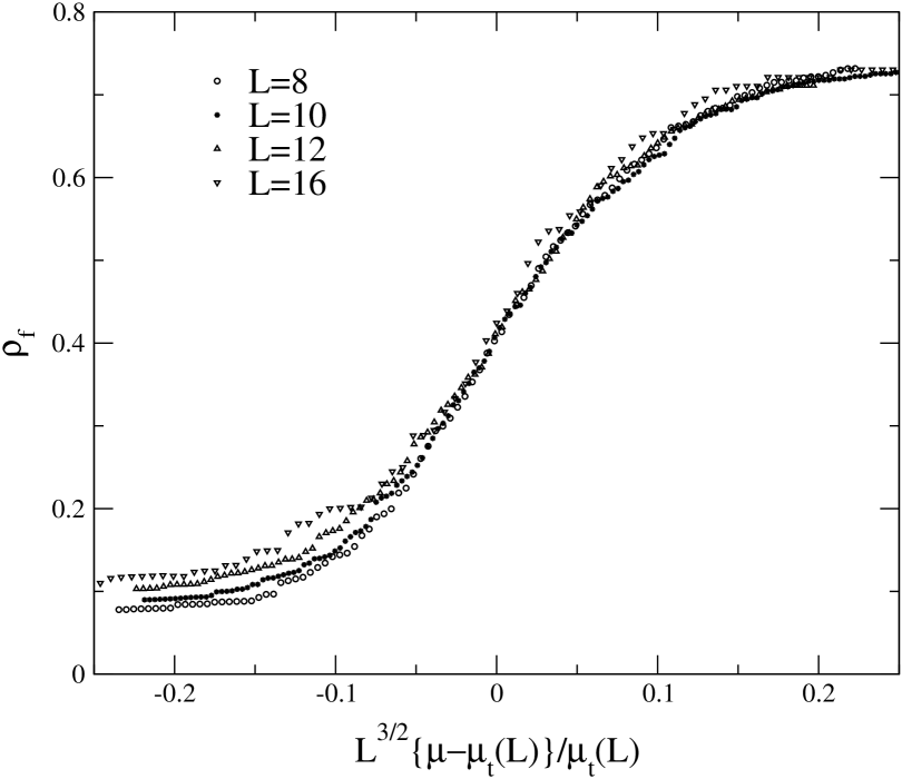
Figure 17: Scaling plot of the average equilibrium isotherms shown in Fig. 16. $\mu_{t}(L)$ is the chemical potential that corresponds to the maximum of the average susceptibility for the system of size $L$.

We thus analyze the curves in Fig. 16 focusing on the transition associated with the largest discontinuity in the individual isotherms. Such a discontinuity in a finite system is of course an artefact of the mean-field approximation: in an exact theory, one would only observe a maximum in the susceptibility, $\chi(\mu)=\partial\rho_{f}^{eq}(\mu)/\partial\mu$ (this is also true with the weighted mean-field theory described above); then, if this maximum occurs at the same $\mu_{t}(L)$ in all matrix realizations $x=\{\eta_{i}\}$ of linear size $L$, the average susceptibility $\chi(\mu_{t})=[\chi(\mu_{t},x)]$ would scale as $L^{3}$ as is usual with first-order phase transitions, e.g., $\chi(\mu)\approx L^{3}F(L^{3}(\mu-\mu_{t}(L))$ around $\mu_{t}(L)$ where $F$ is a (non-universal) scaling funtion. The finite-size scaling behavior of the transition associated with capillary condensation in a disordered solid is however different because every specific sample $x$ is characterized by a different location $\mu_{t}(x,L)$ of the maximum of $\chi(\mu,x)$(or, in the mean-field approximation, a different location of the discontinuity, as can be seen in Fig. 15). According to a standard argument first put forward by BroutB1959 , we expect that all extensive thermodynamic quantities in a disordered system far from criticality are self-averaging, with a Gaussian probability distribution around their mean value and a variance proportional to $L^{-3}$. Although $\mu_{t}(x,L)$ is not the density of an extensive quantity, its value is indirectly determined by the fluctuations of the local random fields, and it seems reasonable (for $L$ large enough and far enough from a critical point) to assume that it also fluctuates around a mean value $\mu_{t}(L)=[\mu_{t}(x,L)]$ with a variance $\delta\mu_{t}(L)^{2}\propto L^{-3}$. This sample-to-sample fluctuation of $\mu_{t}(x,L)$ implies that at a first-order transition the maximum of the average susceptibility should scale as $L^{3/2}$ instead of $L^{3}$. Specifically, we expect that $\chi(\mu)=\partial[\rho_{f}^{eq}(\mu,x)]/\partial\mu\approx L^{3/2}f(L^{3/2}\{\mu-\mu_{t}(L)\})$ around $\mu_{t}(L)$, where $f$ is some (non-universal) scaling function. Our DFT calculations for very weak disorder (e. g., $\rho_{m}=0.1$ and $y=0.6$) strongly support this scaling ansatz, and, as shown in Fig. 17, one can also reach a reasonably good collapse of the equilibrium isotherms for $y=1$, $\rho_{m}=0.25$, and $T^{*}=0.8$ using the scaling reduced variable $L^{3/2}\{\mu-\mu_{t}(L)\}/\mu_{t}(L)$. The curves in Fig. 16 can also be fitted by the function $[\rho_{f}^{eq}(\mu)]=a\tanh(bL^{3/2}\{\mu^{*}-\mu_{t}^{*}(L)\})+c$ where $a,b$ and $c$ are adjustable constants (in both methods, however, there are some deviations for $\mu^{*}<\mu_{t}^{*}(L)$ which we attribute to the presence of the additional discontinuities in the individual isotherms). We thus conclude from this study that a genuine first-order equilibrium transition occurs in the thermodynamic limit for $y=1$, $\rho_{m}=0.25$, and $T^{*}=0.8$.

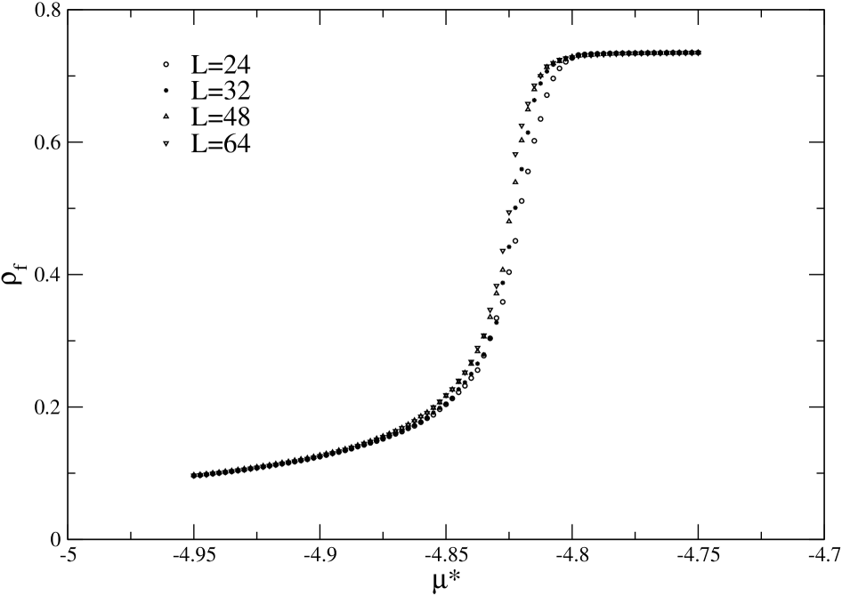
Figure 18: Adsorption isotherm for $y=1.0$ and different system sizes. An average over $50$ $(L=64)$ to $250$ $(L=24)$ matrix realizations has been performed.

Rather remarkably, this transition is not accompanied by a discontinuous behavior on the adsorption branch. Indeed, as can be seen from Fig. 18, for $L$ sufficiently large, the curves collapse onto a clearly continuous isotherm. (Note that we had to consider larger systems than for the equilibrium case in order to reach the asymptotic regime.) The fact that a continuous (but out-of-equilibrium) filling process does not imply the absence of a sharply defined first-order (equilibrium) transition cannot be explained in the traditional picture of capillary condensation based on the independent pore model and is at odds with the common lore in the adsorption community.

V Conclusion

The main conclusion of this study is that most of the phenomenology of capillary condensation in disordered porous solids can be reproduced by a theoretical model that focuses on the properties of a free-energy (or grand potential) landscape with many local metastable states. Thermal fluctuations, which are neglected in the treatment, do not seem to play an important role in usual adsorption experiments, and it is the evolution of the landscape with the gas pressure in the reservoir (or the chemical potential), the temperature, and the amount of disorder (indirectly controlled by the solid porosity and its wettability) that explains the changes in the hysteresis loops and the scanning curves. Fluids in disordered solids are indeed (complicated) experimental realizations of random-field systems for which it is well known that disorder may lead to diverging barriers to relaxation as $T\to 0$FGK1988 . Such externally-driven systems have been extensively studied in recent years at $T=0$ (see, e.g., Refs.S1993 ; VP1994 ), and the present work based on the mean-field density functional theory can be viewed as an extension of such approaches to finite temperatures. In these systems, hysteresis is not the necessary signature of an underlying equilibrium phase transition: this feature is illustrated by the calculations of section IV.B, but is still not well accepted in the adsorption community. As is discussed elsewhereKRT2002 , hysteresis in capillary condensation can also be accompanied by out-of-equilibrium phase transitions whose nature depend crucially on the presence of the external interface between the solid and the gas reservoir.

Figure 5: Check of thermodynamic consistency along the adsorption (a) and desorption (b) isotherms for $y=1.5$ ($L=48$). Circles: average fluid density obtained from the solution of Eqs. (4). Stars: related quantity obtained by differentiating the corresponding grand potential.

References

- (1) The Laboratoire de Physique Théorique des Liquides is the UMR 7600 of the CNRS.
- (2) R. Evans, J. Phys.: Condens. Matter 2, 8989 (1990).
- (3) For a recent review, see L.D. Gelb, K. E. Gubbins, R. Radhakrishnan, and M. Sliwinska-Bartkowiak, Rep. Prog. Phys. 62, 1573 (1999).
- (4) A. Wong and M. Chan, Phys. Rev. Lett. 65, 2567 (1990); A. Wong, S. B. Kim, W. I. Goldburg, and M. H. W. Chan,et al., Phys. Rev. Lett. 70, 954 (1993); D. J. Tulimieri, J. Yoon, and M. H. W. Chan, Phys. Rev. Lett. 82, 121 (1999); L. B. Lurio et al, J. Low Temp. Phys. 121, 591 (2000).
- (5) Z. Zhuang, A. G. Casielles, and D. S. Cannell, Phys. Rev. Lett. 77, 2969 (1996).
- (6) A. J. Brown, Ph.D. Thesis, University of Bristol, 1963; some of Brown’s results are reproduced by G. Mason in Proc. R. Soc. Lond. A 415, 453 (1988), and by P.C. Ball and R. Evans BE1989 .
- (7) S. J. Gregg and K. S. W. Sing, Adsorption, Surface Area and Porosity (Academic Press, London,1982).
- (8) P.C. Ball and R. Evans, Langmuir 5, 714 (1989).
- (9) D. H. Everett, in The Solid Gas Interface, E. A. Flood Ed. (Marcel Dekker, New York, 1967), vol. 2, p. 1055.
- (10) M. P. Lilly and R. B. Hallock, Phys. Rev. B 63, 174503 (2001).
- (11) F. Preisach, Z. Physik 94, 277 (1935).
- (12) E. Pitard, M. L. Rosinberg, G. Stell, and G. Tarjus, Phys. Rev. Lett. 74, 4361 (1995).
- (13) G. C. Wall and R. J. C. Brown, J. Colloid Interface Sci. 82, 141 (1981); G. Mason, J. Colloid Interface Sci. 88, 36 (1982); Proc. R. Soc. Lond. A 390, 47 (1983); A. V. Neimark, Sov. Phys. Tech. Phys. 31, 1338 (1986); M. Parlar and Y. C. Yortsos, J. Colloid Interface Sci. 124, 162 (1988); N. A. Seaton, Chem. Eng. Sci.,46, 1895 (1991); R. A. Guyer and K. R. McKall, Phys. Rev. B 54, 18 (1996).
- (14) E. Kierlik, M.L. Rosinberg, G. Tarjus, and P. Viot, Phys. Chem. Chem. Phys. 3, 1201 (2001).
- (15) E. Kierlik, P. A. Monson, M. L. Rosinberg, L. Sarkisov, and G. Tarjus, Phys. Rev. Lett. 87, 055701 (2001).
- (16) L. Sarkisov, and P. A. Monson, Phys. Rev. E 65, 011202 (2001).
- (17) H.-J Woo and P. A. Monson, preprint (2002).
- (18) see the articles in Spin Glasses and Random Fields, A. P. Young, Ed. (World Scientific, Singapore, 1997).
- (19) E. Kierlik, M. L. Rosinberg, G. Tarjus, and E. Pitard, Mol. Phys. 95, 341 (1998).
- (20) H-J. Woo, L. Sarkisov, and P. A. Monson, Langmuir 17, 7472 (2001).
- (21) F. Detchevery, E. Kierlik, M. L. Rosinberg, and G. Tarjus (in preparation).
- (22) R. B. Stinchcombe, in Phase transitions and critical phenomena, eds. C. Domb and J. L. Lebowitz (Academic Press, London, 1983), vol.7, p. 151.
- (23) The fact that a porous medium exerts spatially varying fields that break the hole-particle symmetry of a lattice gas model (or the up-down symmetry of the equivalent Ising spin model) has also been noted by D. Stauffer and R. B. Pandey, J. Phys. A: Math. Gen. 25, L1079 (1992).
- (24) It should be noted that the hole-particle symmetry of the model is broken even when the probability distribution of the fields is symmetric, i.e., for . It is thus the combination of dilution and random fields that is relevant. The asymmetric random-field Ising model proposed by A. Maritan et al., Phys. Rev. Lett. 67, 1821 (1991), does not include dilution and cannot describe the influence of porosity on the fluid properties.
- (25) D. S. Fisher, G. M. Grinstein, and A. Khurana, Phys. Today 41 (12), 58 (1988).
- (26) Y. Imry and S. K. Ma, Phys. Rev. Lett. 35, 1399 (1975).
- (27) E. Kierlik, M. L. Rosinberg, G. Tarjus, and P. A. Monson, J. Chem. Phys. 95, 264 (1997).
- (28) D. J. Thouless, P. W. Anderson, and R. G. Palmer, Philos. Mag. 35, 593 (1977).
- (29) L. Sarkisov and P. A. Monson, preprint (2002).
- (30) E. Kierlik, M. L. Rosinberg, and G. Tarjus (in preparation)
- (31) D. D Ling, D. R. Bowman, and K. Levin, Phys. Rev. B. 28, 262 (1983).
- (32) D. Lancaster, E. Marinari, and G. Parisi, J. Phys. A: Math. Gen. 28, 3959 (1995).
- (33) R. Mulet, A. Paganani, and G. Parisi, Phys. Rev. B. 63 , 184438 (2001).
- (34) A. A. Middleton, Phys. Rev. Lett. 68, 670 (1992); A. A. Middleton and D. S. Fisher, Phys. Rev. B 47, 3530 (1993).
- (35) J. P. Sethna et al., Phys. Rev. Lett. 70, 3347 (1993).
- (36) This is still a small size compared to those considered in the studies of disordered magnets at (see, e.g., M. C. Kuntz et al., Comp. Sci. Eng. 1, 73 (1999)). This of course is due to the fact that the local densities are not restricted to the values , which forbids the use of bits algorithms and requires large amounts of memory.
- (37) D. Stauffer and A. Aharony, Introduction to Percolation Theory, (Taylor and Francis, London, 1994).
- (38) A. H. Wooters and R. B. Hallock, J. Low Temp. Phys. 121, 549 (2000).
- (39) R. Salazar, R. Toral, and A. Chakrabarti, J. Sol Gel Sci. Technol. 15, 175 (1999).
- (40) Note that the system does not stay in the same minimum along the whole equilibrium isotherm; in a finite-size sample, this results in the small jumps observed in . However, a jump occurs at equilibrium when the grand potentials associated with two local minima cross each other (like in a usual first-order transition) whereas a jump occurs off-equilibrium when a local minimum looses its stability (like at a usual spinodal): for a finite-size sample, and are thus discontinuous curves whereas is continuous.
- (41) C. De Dominicis and A. P. Young, J. Phys. A: Math. Gen. 16, 2063 (1983).
- (42) R. Brout, Phys. Rev. 115, 824 (1959).
- (43) E. Vives and A. Planes, Phys. Rev. B. 50, 3839 (1994); O. Dahmen and J. P. Sethna, Phys. Rev. B 53, 14872 (1996), and references therein.