Theory of Diffusion Controlled Growth

Abstract

We present a new theoretical framework for Diffusion Limited Aggregation and associated Dielectric Breakdown Models in two dimensions. Key steps are understanding how these models interrelate when the ultra-violet cut-off strategy is changed, the analogy with turbulence and the use of logarithmic field variables. Within the simplest, Gaussian, truncation of mode-mode coupling, all properties can be calculated. The agreement with prior knowledge from simulations is encouraging, and a new superuniversality of the tip scaling exponent is both predicted and confirmed.

Diffusion Limited Aggregation (DLA) has accumulated an enormous literature since Witten and Sander first introduced their simulation model of a rigid cluster growing by the accretion of dilute diffusing particles wittensander . The importance of the model is that it encompasses a range of problems where growth or interfacial advance is governed by a conserved gradient flux, that is the local interfacial velocity is given by

$$v_{n}\propto\left|\partial_{n}\phi\right|^{\eta},\qquad\nabla^{2}\phi=0,\text{\qquad}\phi_{\text{interface}}\approx 0$$ (1)

where for DLA $\eta=1$ cargese . The generalisation to a range of positive $\eta$ was introduced by Niemeyer, Pietronero and Wiesmann DBM to model dielectric breakdown patterns, but in this letter we exploit it to support proposed equivalences between models with significantly different ultraviolet cut-off mechanism. Theoretical interest has been fuelled by the fractal and multifractal singularities ; hmp scaling properties of the clusters produced, with controversial claims anomalousscaling ; coniglio89 ; mandelbrot (and counter-claims counterclaims ; somfai99 ; noisereduction ) of anomalous scaling, and by the longstanding absence here resolved of an overall theortical framework to understand the problem.

The presence of a cut-off lengthscale $a$ below which the physics dictates smooth growth is a crucial ingredient of DLA; it is known that otherwise infinitely sharp cusps develop in the interface within finite time bensimonshraiman . In DLA this cutoff is fixed and set by the size of accreting particles, but there are other problems where it is set in a more subtle dynamical way by the surface boundary conditions on the diffusion field. In dendritic soldification this comes about through competition between surface energy and diffusion kinetics (with $\eta=1$), leading to

$$a\propto\left|\partial_{n}\phi\right|^{-m}$$ (2)

with $m=1/2$ at least for those tips not in retreat langer . In terms of $m$, simple DLA corresponds to $m=0$, and in the theory below in two dimensions we will map onto the case where $a$ is such that each growing tip has fixed integrated flux, corresponding to $m=1$.

It is central to fractal (and multifractal) behaviour in DLA that the measure given by the diffusion flux [density] $\partial_{n}\phi$ onto the interface has singularities hmp ; singularities , such that the integrated flux onto the growth within distance $r$ of a singular point is given by

$$\mu(r)\sim r^{\alpha}.$$ (3)

Applying this phenomenology to the scaling around growing tips, we can establish an equivalence between models at different $\eta$ and $m$ by requiring that the relative advance rates of different growing tips are matched. Consider two competing tips labelled $1,2$, for two growths with the same overall geometry but growing governed by parameters $(\eta,m)$ and $(\eta^{\prime},m^{\prime})$ respectively. For tip 1 we will have tip radius $a_{1}$ and flux density $j_{1}$ which are matched between the two different models by $j_{1}^{\prime}a_{1}^{\prime d-1}/a_{1}^{\prime\alpha}=j_{1}a_{1}^{d-1}/a_{1}^{\alpha}$ and similarly for tip 2, whilst the two tips are interrelated by $a_{1}^{\prime}j_{1}^{\prime m^{\prime}}=a_{2}^{\prime}j_{2}^{\prime m^{\prime}}$ and similarly for the unprimed quantities. If we insist that their advance velocities are in the same ratio in both models this requires $(j_{1}/j_{2})^{\eta}=(j_{1}^{\prime}/j_{2}^{\prime})^{\eta^{\prime}}$, which forces the parameter relation

$$\frac{1+m(1+\alpha-d)}{\eta}=\frac{1+m^{\prime}(1+\alpha-d)}{\eta^{\prime}}.$$ (4)

For the two models to be equivalent in the relative velocities of all tips requires their parameters be related as above, where $\alpha$ is the singularity exponent associated with growing tips which we take to be the same as we are matching the geometry at scales above the cut-offs.

Although we have not strictly proved the equivalence of the models related above, we have shown that any such relationship must follow Eq. (4) and we will assume in the rest of this letter that this equivalence holds. All such models are then classifiable in terms of a convenient reference such as $\eta_{0}$, the equivalent $\eta$ when $m=0$, corresponding to the original Dielectric Breakdown Model. For example dendritic solidification with $\eta=1$ and $m=1/2$ corresponds to $\eta_{0}=\frac{2}{3+\alpha-d}$: it is thus not equivalent to DLA, but to another member of the DBM class. Another puzzle resolved by our classification is a recent study showing conflicting scaling between DLA and different limits of a ’laplacian growth’ model laplaciangrowthmodel . In the present terminology the latter model corresponds to $m=-1$ and its two limits of low and high coverage of the growing surface per growth step have $\eta=3$ and $\eta=1$ respectively. Using $\alpha=0.7$ (see below) these map through Eq. (4) into $\eta_{0}=2.31$ and $\eta_{0}=0.77$ respectively, so the way their scaling brackets that of DLA is quite expected.

DLA and DBM have hitherto been regarded as models in statistical physics, in that the local advance rate in Eq. (1) has been implemented as the probabilty per unit time for the growth locally to make some unit of advance, entailing an inherent shot noise. Here we argue that diffusion controlled growth is a problem of turbulence type, with noise self-organising from minimal input. The data in Fig. 1 show how the relative fluctuations can approach their limiting value from below as well as from above.

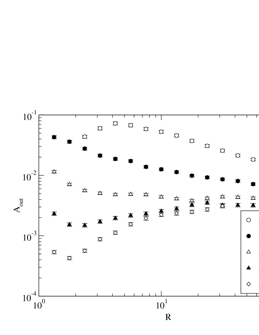
Figure 1: The size fluctuations (“output noise”) $A_{\text{out}}=(\delta N/N)^{2}$, measured at fixed radius $R$ for DLA clusters grown with off-lattice noise reduction noisereduction at various (“input”) noise levels $A_{\text{in}}$. For low $A_{\text{in}}$, $A_{\text{out}}$ self organizes from below in the manner of a turbulent system.

The new ideas above, that we can balance changing the cut-off exponent $m$ by adjustment of $\eta$, and that noise can be left to self organise,  are the key to a new theoretical formulation of the problem, at least in two dimensions of space to which we now specialise. In two dimensions the Laplace equation in (1) can be solved in terms of a conformal transformation between the physical plane of $z=x+iy$ and the plane of complex potential $\omega=\phi+i\theta$ in which we take the growing interface to be mapped into the periodic interval $\theta=[0,2\pi),\phi=0$ and the region outside of the growth mapped onto $\phi>0$. Then adapting reference bensimonshraiman , we have for the dynamics of the interface following Eq. (1),

$$\frac{\partial z(\theta)}{\partial t}=-i\frac{\partial z}{\partial\theta}\mathcal{P}\bigg{[}\left|\frac{\partial\theta}{\partial z}\right|^{1+\eta}\bigg{]}.$$ (5)

The linear operator $\mathcal{P}$ is most simply described in terms of Fourier transforms: $\mathcal{P}[\sum_{k}e^{-ik\theta}f_{k}]=\sum_{k}P[k]e^{-ik\theta}f_{k}=f_{0}+2\sum_{k=1}^{K}e^{-ik\theta}f_{k}$, where we have introduced here an upper cut-off wavevector $K$. It is easily shown that on scales of $\theta$ greater than $K^{-1}$ a smooth interface is linearly unstable with respect to corrugation for $\eta>0$ (the Mullins-Sekerka instability mullinssekerka ), whereas for scales of $\theta$ less than $K^{-1}$ the equation drives smooth behaviour (corresponding locally to the case $\eta=-1$). This cutoff on a scale of $\theta$, the cumulative integral of flux, corresponds in terms of tip radii and flux densities to $aj\thickapprox K^{-1}$, that is an $m=1$ cutoff law. Thus the parameter $\eta$ in Eq. (5) is more specifically $\eta_{1}=\alpha\eta_{0}$, using Eq. (4) with $d=2$.

We have made a numerical test of Eq. (5) and the equivalence (4), with disorder supplied only through the initial condition, by applying them to the case of growth along a channel with periodic boundary conditions (cylinder). For this case analyticity of the conformal map requires that $z(\theta)=i\theta+\sum_{k\geq 0}z_{k}e^{-ik\theta}$ and the overall advance rate of the growth reduces to $\frac{\partial z_{0}}{\partial t}=\left(\left|\frac{\partial\theta}{\partial z}\right|^{1+\eta_{1}}\right)_{0}$, which we can compare to the expected scaling of tip velocity with the cutoff, $v\thicksim K^{(1-\alpha)\eta_{1}/\alpha}$. It is convenient to change variables to $\psi=(\partial z/\partial\theta)^{-(1+\eta_{1})/2}$, in terms of which we obtain

$$\frac{\partial\psi}{\partial t}=-i\frac{\partial\psi}{\partial\theta}\mathcal{P}[\psi\overline{\psi}]+iy\psi\frac{\partial}{\partial\theta}\mathcal{P}[\psi\overline{\psi}]$$ (6)

where $y=(1+\eta_{1})/2$ and the tri-linear form of the RHS enables us to compute numerically the motion within a purely Fourier representation. Figure 2 shows the measured variation of $\sum_{j<k}\left|\psi_{j}\right|^{2}$ vs $k^{\eta_{1}}$: this is expected to exhibit a power law with exponent $(1/\alpha-1)$ and the observed slope plotted in this way is surprisingly independent of $\eta_{1}$.

The most important result of our numerical study of Eq. (6) is that this clearly does self-organise into statistical scaling behaviour, given disorder from only the initial conditions. However the numerical results are also remarkable, as we obtain $\alpha\approx 0.74\pm 0.02$ with no significant dependence on $\eta_{1}$ in the range studied. This not only agrees reasonably with the value $\alpha=D-1=0.71$ known from large direct simulations of DLA DLAdimension ; channelxsi , but also appears to imply a deeper unversality which we will see is replicated in our analytic theory below.

Figure 2: Cumulative contribution to the mean growth velocity plotted against wavevector as $k^{\eta_{1}}$with logarithmic scales. The data are (bottom to top) for $\eta_{1}=0.5,0.6,0.7,0.8,0.9,1.0$ and all exhibit a common power law slope $1/\alpha-1\approx 0.35\pm 0.04$ per the guidelines shown.

We now turn to a theoretical analysis of Eq. (5), for which a primary requirement is that we must obtain results explicitly independent of the cut-off as $K\rightarrow\infty$. This is hard because we have already seen that the mean advance rate of the interface diverges as a power of $K$, and on fractal scaling grounds one would expect the same divergent factor to appear in the rate of change of simple variables such as $z_{k}$ or $\psi_{k}$. One can of course take ratios of rates of change and look to order terms such that divergences cancel, but to make this work we have been forced to introduce yet another change of variables,

$$-i\frac{\partial z}{\partial\theta}=\exp\left(-\lambda(\theta)\right)=\exp\left(-\sum_{k>0}\lambda_{k}e^{-ik\theta}\right),$$ (7)

which corresponds to Fourier decomposing the logarithm of the flux density. The key to the success of these variables is that they decompose the flux density itself multiplicatively and, as we shall see, quite naturally capture its multifractal behaviour. In terms of these ’logarithmic variables’ the equation of motion becomes

$$\frac{\partial\lambda_{k}}{\partial t}=-\sum_{j\leq k}(k-j)\lambda_{k-j}P(j)\left(e^{y(\lambda+\overline{\lambda})}\right)_{j}+2k\left(e^{y(\lambda+\overline{\lambda})}\right)_{k}$$ (8)

where subscripts on bracketed expressions imply the taking of a Fourier component, by analogy with $\lambda_{k}$. The advance rate of the mean interface is given in these variables by $\frac{\partial z_{0}}{\partial t}=\left(e^{y(\lambda+\overline{\lambda})}\right)_{0}$.

Now let us suppose some ignorance of the initial conditions and describe the system in terms of a joint probability distribution over the $\lambda_{k}$, and let us denote averages over this [unknown] distribution by $\left\langle..\right\rangle$. We can in principle determine the distribution through its moments, whose evolution we now compute. For simplicity we assume translational invariance with respect to $\theta$, so that only moments of zero total wavevector need be considered, of which the lowest gives: $\frac{\partial}{\partial t}\left\langle\lambda_{k}\overline{\lambda}_{k}\right\rangle=\left(-\sum\limits_{j\leq k}(k-j)P(j)\left\langle\lambda_{k-j}\overline{\lambda}_{k}e_{j}^{y(\lambda+\overline{\lambda})}\right\rangle+2k\left\langle\overline{\lambda}_{k}e_{k}^{y(\lambda+\overline{\lambda})}\right\rangle\right)+\left(\text{c. conj.}\right)$. All of the higher moments lead to the same form of averages on the RHS, $\left\langle\text{multinomial(}\lambda,\overline{\lambda}\text{)}e^{y(\lambda+\overline{\lambda})}\right\rangle$, and all of these terms are conveniently expressed in terms of cumulants cumulants , using the identities $\left\langle Xe^{W}\right\rangle/\left\langle e^{W}\right\rangle=\left\langle Xe^{W}\right\rangle_{c}$, $\left\langle XYe^{W}\right\rangle/\left\langle e^{W}\right\rangle=\left\langle XYe^{W}\right\rangle_{c}+\left\langle Xe^{W}\right\rangle_{c}\left\langle Ye^{W}\right\rangle_{c}$, etc. The key helpful feature is that the expressions we require all naturally divide by one factor of $\left\langle e^{y(\lambda+\overline{\lambda})}\right\rangle=\frac{\partial}{\partial t}\left\langle z_{0}\right\rangle$, which is what we sought in order to remove divergences.

To obtain tractable results we need to introduce some closure approximation(s) and we present here the simplest, neglecting all cumulants higher than the second, equivalent to assuming a joint Gaussian distribution (of zero mean) for $\lambda$. This is entirely characterised by its second moments $S(k)=\left\langle\lambda_{k}\overline{\lambda}_{k}\right\rangle$ which by Eq. (8) we find evolve according to $\partial S(k)/\partial\left\langle z_{0}\right\rangle=-kS(k)-y^{2}kS(k)^{2}-2y^{2}\sum_{j<k}jS(j)S(k)+2ykS(k)$. This in turn approaches a stable steady state solution where

$$S(k)=\frac{2y-1}{y^{2}}k^{-1}\,,\quad k\text{ odd;}\quad\,\,S(k)=0\,,\quad k\text{ even.}$$ (9)

The absence of even $k$ is readily interpreted in terms of the dominance of one major finger and one major fjord.

Within the Gaussian approximation and its predicted variances (9) we can now compute all [static] properties of diffusion controlled growth, in a channel and (see later discussion) also in radial geometry. The multifractal spectrum of the harmonic measure follows from computing the general moment hmp $\left\langle\left|\frac{\partial\theta}{\partial z}\right|^{-\tau}\right\rangle=\left\langle e^{(\lambda+\bar{\lambda})\tau/2}\right\rangle=\exp\left(\tau^{2}/4\sum_{k}^{K}S(k)\right)\simeq K^{q(\tau)-1-\tau}$, leading to

$$q(\tau)=1+\tau+\tau^{2}\frac{\eta_{1}}{2\left(1+\eta_{1}\right)^{2}}$$ (10)

and it is easy to see that any closure scheme based on keeping cumulants of $\lambda$ up to some finite order leads to a polynomial truncation of $q(\tau)$. From the Legendre Transform of the inverse function $\tau(q)$ we obtain the corresponding spectrum of singularities,

$$f(\alpha)=2-\frac{1}{\alpha}+\frac{1}{2}\left(\eta_{1}+\frac{1}{\eta_{1}}\right)\left(2-\alpha-\frac{1}{\alpha}\right)$$ (11)

which in Fig. 3 is compared to measured data for DLA f(a)data , which later measurements jensen02 reinforce. For the region of active growth $\alpha\leq 1$ ($q\geq 0$) the theory is quantitatively accurate. At $\alpha=1$ it conforms to Makarov’s theorem makarov , and in contrast to the Screened Growth Model screenedgrowth it does this without adjustment. For $\alpha>1$ the spectrum only qualitatively the right shape, and for such screened regions our equations based on tip scaling may not hold.

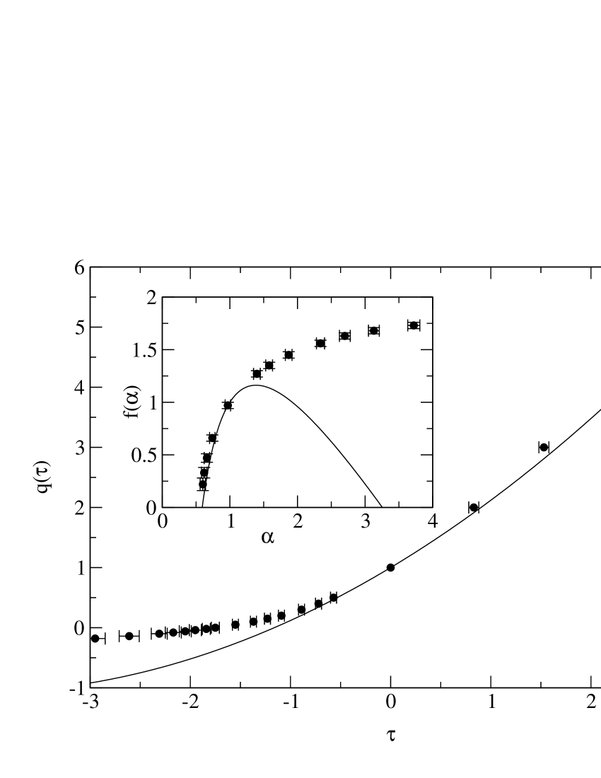
Figure 3: Multifractal spectra from the Gaussian theory ($\alpha=2/3$), compared to measured values for DLA f(a)data . Agreement is excellent for the active region $\tau\geq 0$, $\alpha\leq 1$, and there are no adjustable parameters.

Although the multifractal moments depend significantly on the input parameter $\eta_{1}$, the tip scaling exponent $\alpha$ turns out to be independent of this and in close agreement with our numerical results. Matching the expected scaling of the mean velocity (as used to measure $\alpha$ above) to that of the multifractal moment with $\tau=-(1+\eta_{1})$ leads direcly to $\alpha=2/3$ independent of $\eta_{1}$. This is a remarkable success for the Gaussian Theory to predict this hitherto unexpected result so closely.

The multifractal spectrum suggests that the Gaussian approximation is good in the growth zone, so we have computed the penetration depth as a further test. For growth in the channel we define relative penetration depth $\Xi$ as the standard deviation of depth $\Re(z)$ along the chanel, computed over the harmonic measure, divided by the width of the channel. This leads to $\left(2\pi\Xi\right)^{2}=\left\langle z\overline{z}\right\rangle/2=\sum_{k>0}k^{-2}\left\langle\left|e_{k}^{\lambda}\right|^{2}\right\rangle/2$ where the required averages can all be computed in the approximation of Gaussian distributed $\lambda$. Using $\eta_{1}=2/3$ corresponding to DLA this leads to $\Xi_{\text{theory}}=0.13$,  compared to $\Xi_{\text{DLA}}=0.14$ from direct simulations of DLA growth in a periodic channel channelxsi .

All of the new theory is readily extended to growth from a point seed in radial geometry. The multifractal spectrum turns out to be unchanged, in accordance with expectations from universality. The penetration depth relative to radius gives $\Xi_{\text{theory}}=0.20$ for radial DLA, compared to our recently published extropolation from simulations, $\Xi_{\text{DLA}}=0.13$ somfai99 .

For DLA and its associated Dielectric Breakdown Models we have shown a theoretical framework which is complete in the sense that essentially all measurable quantities can be calculated. For amplitude factors such as the relative penetration depth there is no theoretical precedent. For the full spectrum of exponents the advance over the Screened Growth Model is the elimination of fitting parameters. For the exponent $\alpha_{\text{tip}}$ we have in the Gaussian approximation a striking new result that this is independent of $\eta$, which begs direct confirmation by (expensive) particle-based simulations. However for DLA in particular we have not yet improved on the best theoretical value of $\alpha_{\text{tip}}$, which remains $1/\sqrt{2}\approx 0.71$ from the Cone Angle Approximation coneangle .

Within DLA and DBM we look forward to calculating more properties such as the response to anisotropy, which is fairly readily incorporated into our equations of motion. A more challenging avenue is to improve on the Gaussian approximation which we have used to obtain explicit theoretical results. Truncating at a cumulant of higher order than the second is hard, and more seriously it does not correspond to a positive (semi-)definite probability distribution. An alternative route of improvement which we are exploring is closure at the level of the full multifractal spectrum.

There are possibilities for wider application of ideas in this letter, where we have formulated DLA and DBM as a turbulent dynamics governed by a complex scalar field in 1+1 dimensions. Decomposing this field multiplicatively (through Fourier representation of its logarithm) was the crucial step to obtain renormalisable equations and theoretical access to the multifractal behaviour, even though other representations offered equations of motion (6) with weaker non-linearity. It is natural to speculate whether the same strategy might apply to turbulent problems more widely, where the key issue appears to be identifying suitable fields to decompose multiplicatively which are of local physical significance, and subject to closed equations of motion.

- (1) T.A. Witten and L.M. Sander, Phys. Rev. Lett. 47, 1400 (1981).
- (2) R. C. Ball, in On Growth and Form, edited by H. E. Stanley and N. Ostrowski (Martinus Nijhof, Dordrecht, 1986) pp. 69–78.
- (3) L. Niemeyer, L. Pietronero and H.J. Wiesmann, Phys. Rev. Lett. 52, 1033 (1984).
- (4) C. Amitrano, A. Coniglio, P. Meakin and M. Zannetti, Phys.Rev. B 44, 4974 (1991).
- (5) T.C. Halsey, P. Meakin and I. Procaccia, Phys. Rev. Lett. 56, 854 (1986).
- (6) M. Plischke and Z. Rácz, Phys. Rev. Lett. 53, 415 (1984).
- (7) A. Coniglio and M. Zannetti, Physica D 38, 37 (1989).
- (8) B. B. Mandelbrot, B. Kol, and A. Aharony, Phys. Rev. Lett. 88, 055501 (2002).
- (9) P. Meakin and L.M. Sander, Phys. Rev. Lett. 54, 2053 (1985)
- (10) E. Somfai, L.M. Sander and R.C. Ball, Phys. Rev. Lett. 83, 5523 (1999).
- (11) R.C. Ball, N.E. Bowler, L.M. Sander and E. Somfai, eprint cond-mat/0108252, submitted to Phys. Rev. E.
- (12) B. Shraiman and D. Bensimon, Phys. Rev. A 30, 2840 (1984).
- (13) J.S. Langer, Rev. Mod. Phys. 52, 1 (1980).
- (14) F. Barra, B. Davidovitch, A. Levermann and I. Procaccia, Phys. Rev. Lett. 87, 134501 (2001).
- (15) W.W. Mullins and R.F. Sekerka, J. Appl. Phys. 34, 323 (1963).
- (16) P. Ossadnik, Physica A 176, 454 (1991).
- (17) E. Somfai, R.C. Ball and L.M. Sander, (in preparation).
- (18) R. Kubo, J. Phys. Soc. Japan 17, 1100 (1962).
- (19) R.C. Ball and O.R. Spivack, J. Phys. A. (Lond) 23, 5295 (1990).
- (20) M.H. Jensen, A. Levermann, J. Mathiesen, I. Procaccia, Phys. Rev. E 65, 046109 (2002).
- (21) N.G. Makarov, P. Lond. Math. Soc. 51, 369 (1985).
- (22) T.C. Halsey and M. Leibig, Phys. Rev. A 46, 7793 (1992).
- (23) R.C. Ball, Physica A 140, 62 (1986).