Non-commutative Chern-Simons for
the Quantum Hall System and Duality

Abstract

The quantum Hall system is known to have two mutually dual Chern-Simons descriptions, one associated with the hydrodynamics of the electron fluid, and another associated with the statistics. Recently, Susskind has made the claim that the hydrodynamic Chern-Simons theory should be considered to have a non-commutative gauge symmetry. The statistical Chern-Simons theory has a perturbative momentum expansion. In this paper, we study this perturbation theory and show that the effective action, although commutative at leading order, is non-commutative. This conclusion is arrived at through a careful study of the three-point function of Chern-Simons gauge fields. The non-commutative gauge symmetry of this system is thus a quantum symmetry, which we show can only be fully realized only through the inclusion of all orders in perturbation theory. We discuss the duality between the two non-commutative descriptions.

I Introduction

Fractional quantum Hall (FQH) states are topological quantum fluid phases of two-dimensional electron gases in large magnetic fields. These incompressible fluid states have universal wave functions, the Laughlin wave functions laughlin and their hierarchical extensions haldane-hierarchy ; halperin-hierarchy ; jain , and their associated spectrum of low-energy excitations have universal quantum numbers, such as their charge and statistics. Smooth short-distance changes in the precise form of the electron-electron interactions do not change the universal properties of these ground states and of their low energy spectra. On closed surfaces, the ground states of FQH systems exhibit degeneracies which are a direct manifestation of the topological nature of these fluid states wen-niu ; wen-topo .

The universal properties of FQH states can also be described in the form of an effective quantum field theory for the degrees of freedom with energies low compared to the cyclotron energy $\hbar\omega_{c}$ and/or the Coulomb energy $e^{2}/(\epsilon\ell)$ (whichever is smallest), and at distances long compared to the magnetic length $\ell=\sqrt{\hbar c/eB}$ (and/or any other short distance scale related to the interaction). The low energy theory of the FQH states is a Chern-Simons gauge theory. There are two equivalent, mutually dual, descriptions of this effective theory. In the first, the Chern-Simons gauge theory is derived directly from a theory of interacting electrons zhk ; lopez-fradkin-91 ; zhang , and the gauge field is the statistical gauge field. The second description is based on a hydrodynamic picture blok-wen ; wen-review ; wen-zee-matrix ; frohlich-zee ; frohlich-kerler ; bahcall-susskind . In this picture the gauge fields embody the conserved charge densities and currents of the electron fluid. Naturally, both descriptions, which are dual to each other, yield an effective action for slowly varying electromagnetic gauge fields which also has a Chern-Simons form, a result required by gauge invariance and broken time-reversal symmetry. Thus Chern-Simons gauge field theories appear as the natural field-theoretic description of the low energy physics of FQH states.

In Ref. Suss , Susskind argued that quantum Hall systems are inherently non-commutative, and that their effective field theory should be a non-commutative extension of the Chern-Simons gauge theory. From a heuristic point of view, this is expected, because of the non-commutative magnetic algebra of the quantum mechanics of electrons in a magnetic field girvin-jach . Thus, when acting on the Hilbert space of excitations of an incompressible (gapped) state, physical observables such as the charge and current densities, obey a local extension of the magnetic algebra girvin-jach , a magnetic current algebra related to the $W_{\infty}$ symmetry of area preserving diffeomorphisms sakita ; stone ; ctz . The physical observables of this magnetic current algebra obey Moyal products controlled by the magnetic length $\ell$.

The non-commutative gauge theory that Susskind discusses is an effective hydrodynamic theory of the fractional quantum Hall states. Thus, as such it describes only the low energy physics of these incompressible fluid states. It is an extension of the conventional effective Chern-Simons descriptions which have been used quiet successfully to describe interesting phenomena such as edge states. Susskind’s non-commutative hydrodynamics is a natural extension of these theories. However, Susskind’s proposal poses a number of questions. For instance, the non-commutativity of Susskind’s theory, at the level of the effective action of Ref. Suss , is controlled not by the magnetic length $\ell$, but instead by the particle density $\rho$ (or rather, by the mean separation between the electrons). It is thus natural to inquire what is the connection between Susskind’s non-commutative Chern-Simons gauge theory and the magnetic current algebra as they superficially appear to be controlled by different (although obviously related) non-commutativity parameters. On the other hand, since the non-commutativity happens on such a short-distance scale, it is also necessary to explain in what sense this theory is robust, i.e., insensitive to other non-universal short distance physical phenomena not considered in this theory. For instance, at short distances the particular form of the interaction matters since it is what determines how big the energy gaps are and how fast do the excitations move. We will see below that what is special about the non-commutativity is that it is the only short distance effect associated with the broken time-reversal symmetry and parity of electrons in magnetic fields, and that in this sense this structure is robust. Nevertheless, the effects of non-commutativity show up primarily in non-uniform states and in practice both the time-reversal even and odd processes are important. For example, it is well known from the classic work of Girvin, MacDonald and Platzman gmp that the spectrum of collective modes with a finite length scale, such as the roton modes, is due to a combination of the magnetic algebra and electron-electron interaction effects.

In this paper, we provide a complementary derivation of Susskind’s result, based directly on the field theory of interacting electrons coupled to gauge fields. Our calculation is an extension of the standard methods of Ref. lopez-fradkin-91 , which were used before to derive the conventional Chern-Simons effective gauge theory and the universal physics they contain: the values of the quantum Hall conductivity for which the FQH state is stable, the ground state degeneracy, and the quantum numbers of the excitations. Here we will show that a non-commutative Chern-Simons gauge theory emerges naturally within this framework. We will find that to lowest order of approximation, the non-commutativity parameter does not agree with the one found by Susskind. However, we will show that Susskind’s result is required by the constraints imposed by the magnetic current algebra of the charge densities and currents. Hence, higher order quantum corrections lead to finite renormalizations of the effective non-commutativity parameter. In contrast the level of the Chern-Simons theory is not renormalized beyond its Gaussian value, due to the constraints of topological and gauge invariance, and incompressibility. We will show that these results are universal in the sense that these are the only effects at this length scale which are odd under time-reversal (and parity).

Throughout the paper, we shall use the following notation:

$$a_{\mu}: {\rm statistical\ CS\ gauge\ field}$$

$$b_{\mu}: {\rm hydrodynamic\ CS\ gauge\ field}$$

$$A_{\mu}: {\rm electromagnetic\ gauge\ field}$$

The paper is organized as follows. In Section II, we briefly review Susskind’s fluid dynamics derivation of non-commutative Chern-Simons theory for the Laughlin FQH states. In Section III, we review the derivation of commutative Abelian Chern-Simons theory for the FQH states in the Jain sequences, based on the notion of flux attachment, as the effective field theory of FQH states. In Section IV, we present the results of our calculation of the effective gauge field action, obtained by integrating out fermions. The bulk of this calculation, as well as notational details are relegated to Appendix A. In Section V, we discuss the non-commutative version of Chern-Simons duality. Here we discuss the connection between non-commutative Chern-Simons theory, the underlying magnetic algebra and the $W_{\infty}$ algebra of the currents. Finally, in Section VI we present our conclusions.

II Hydrodynamic Chern-Simons Theory and Non-Commutativity

Susskind’s discussion concerns the hydrodynamic Chern-Simons field. We briefly review that derivation here, largely to establish notation. In the hydrodynamic limit, we have a charged fluid of number density $\rho$ in a magnetic field $B$. A fluid element is labeled by coordinates $x^{a}(y)$, the $y^{i}$ being co-moving coordinates. The Lagrangian is taken to be

$${\cal L}=\int d^{2}y\ \rho_{0}\left(\frac{M}{2}\dot{x}_{a}^{2}-\frac{eB}{2}\epsilon_{ab}x^{a}\dot{x}^{b}-V(\rho)\right).$$ (1)

The gauge generators are of the form

$$G = \frac{1}{M}\int d^{2}y\,\pi_{a}\delta x^{a}$$

$$= \rho_{0}\int d^{2}y\,\Lambda(y)\frac{\partial}{\partial y^{i}}\left[\epsilon^{ij}\left(\dot{x}_{a}+\frac{\omega_{c}}{2}\epsilon_{ab}x^{b}\right)\frac{\partial x^{a}}{\partial y^{j}}\right]$$

where $\zeta^{i}(y)=\epsilon^{ij}\partial_{j}\Lambda$ is the transformation of $y^{i}$. This symmetry, when restricted to the lowest Landau level, reduces to area preserving diffeomorphisms (APD) in space. The conservation of $G$ implies that

$$V_{\Sigma}+\frac{e}{M}\Phi_{\Sigma}={\rm constant}$$ (3)

where $V_{\Sigma}$ is the vorticity and $\Phi_{\Sigma}$ is the magnetic flux through a region $\Sigma$.

Assuming that the fluid is near static equilibrium at $\rho\simeq\rho_{0}$, we may expand

$$x^{a}=y^{a}+\theta\epsilon^{ab}{b}_{b}(y)$$ (4)

where $\theta\equiv 1/2\pi\rho_{0}$. The Lagrangian becomes

$${\cal L}=\frac{M\theta}{4\pi}\int d^{2}y\,\left[\omega_{c}\epsilon^{ij}\dot{b}_{i}{b}_{j}+\dot{b}_{i}^{2}-c_{s}^{2}(\nabla\times{b})^{2}\right]$$ (5)

while eq. (3) becomes

$$\frac{e}{M}\Phi_{0}+\omega_{c}\theta\oint{b}-\theta^{2}\oint d{b}_{i}\left(\dot{b}^{i}+\frac{\omega_{c}}{2}\epsilon^{ij}{b}_{j}\right)=\rm{constant}$$ (6)

In the vacua of interest, the vorticity vanishes, and we find the constraint

$$\epsilon^{ij}\frac{\partial}{\partial y^{j}}\left[\omega_{c}{b}_{i}-\theta\left(\dot{b}^{k}+\frac{\omega_{c}}{2}\epsilon^{kl}{b}_{l}\right)\frac{\partial{b}_{k}}{\partial y^{i}}\right]=0$$ (7)

This may be enforced by introducing a Lagrange multiplier ${b}_{0}$, and consequently, we find that the action is (at leading order in powers of $B$)

$$S=\frac{\hbar\theta}{4\pi\ell^{2}}\int d^{3}y\ \epsilon^{\mu\nu\rho}\left[{b}_{\mu}\partial_{\nu}{b}_{\rho}+\frac{\theta}{3}\epsilon^{ij}\partial_{i}{b}_{\mu}\partial_{j}{b}_{\nu}{b}_{\rho}\right]$$ (8)

Now the supposition is that this action should be interpreted as the leading term in a momentum expansion of

$$S_{NCCS}=\hbar\frac{k}{4\pi}\int d^{3}y\,\epsilon^{\mu\nu\lambda}\left({b}_{\mu}\star\partial_{\nu}{b}_{\lambda}-\frac{2i}{3}{b}_{\mu}\star{b}_{\nu}\star{b}_{\lambda}\right)$$ (9)

where the $\star$-product is

$$f(x)\star g(x)=\left.\exp\left\{\frac{i}{2}\theta\epsilon^{ij}\frac{\partial}{\partial y^{i}}\frac{\partial}{\partial z^{j}}\right\}f(y)g(z)\right|_{y=z=x}$$ (10)

Thus the field $b_{\mu}$ is a (hydrodynamic) non-commutative Abelian Chern-Simons gauge field. The non-commutativity is controlled here by the parameter $\theta=1/2\pi\rho_{0}=\ell^{2}/\nu$. If we couple this to the electromagnetic potential and compute the Hall conductance, we find that the filling fraction is given by $\nu=1/k$. Hence, this theory describes the quantum hydrodynamics of fractional quantum Hall states in the Laughlin sequence $\nu=1/k$, with $k$ an odd integer.

III Duality Invariant Formalism: Commutative Limit

Now let us review the dual Chern-Simons pictures of the FQH states following the arguments of Ref. chetan and Ref. lopez-fradkin-98 . Let us describe the problem of electrons in a large magnetic field in a Feynman path-integral picture. We will denote the histories of the electrons in $2+1$-dimensional space-time by a set of conserved $3$-currents $j_{\mu}$ (with $\mu=0,1,2$). Let us write the (fermionic) path-integral in the form of a sum over current configurations (i. e. a sum over the histories of the particles)

$$Z=\sum_{[j]}e^{\displaystyle{iS[j]/\hbar-i\frac{e}{\hbar c}\int d^{3}x\ A_{\mu}j^{\mu}+i\phi[j]}}$$ (11)

where $\phi[j]$ is a phase which accounts for the statistics of the particles. Here, $S[j]$ is the action for $N$ interacting fermions, $A_{\mu}$ is the external magnetic field.

Next, we note that for every configuration of currents $[j]$ it is possible to compute the linking number $\nu_{L}([j])$ of the configuration, which is a topological invariant and it is an integer. (Technically this requires the assumption that the currents do not cross or equivalently that there is a “hard core” condition.) The expression of $\nu_{L}[j]$ in terms of $j$ is known as the Gauss invariant, which is non-local:

$$\nu_{L}[j]=\int\int j\wedge\partial^{-1}\cdot j$$ (12)

We will express the fact that the currents $j_{\mu}$ are conserved, i.e. $\partial\cdot j=0$ by introducing wen-review a hydrodynamic field $b$, related to the particle current by

$$j^{\mu}=\frac{1}{2\pi}\epsilon^{\mu\nu\lambda}\partial_{\nu}b_{\lambda}$$ (13)

which we will denote in short hand form as $j=\frac{1}{2\pi}\partial\wedge b$.

When written in terms of $b$, the link invariant is local and it has a Chern-Simons form wilczek-zee ; wu-zee :

$$\nu_{L}[j]=\frac{1}{4\pi^{2}}\int d^{3}x\;b\cdot\partial\wedge b$$ (14)

Hence, for any arbitrary integer $n$, we can shift the action $S[j]\to S[j]+2\pi in\hbar\nu_{L}[j]$ without changing any quantum mechanical amplitude.

To enforce current conservation, we insert $b_{\mu}$ into the partition function by making use of the identity

$$1=\int[Db]\;\delta\left(j-\frac{1}{2\pi}\partial\wedge b\right)=\int[Db][Da]\;\;e^{\displaystyle{i\int\;d^{3}x\;a\cdot\left(j-\frac{1}{2\pi}\partial\wedge b\right)}}$$ (15)

To represent the $\delta$-function, we have introduced another vector field $a$. Thus, we may write the full fermionic path integral in the equivalent form

$$Z=\int[Db][Da]\sum_{[j]}e^{\displaystyle{iS[j]/\hbar+i\phi[j]+i\int d^{3}x\left((a-\frac{eA}{\hbar c})\cdot j-\frac{1}{2\pi}a\cdot\partial\wedge b+\frac{2n}{4\pi}b\cdot\partial\wedge b\right)}}$$ (16)

Hence, a system of interacting fermions in an external electromagnetic field is equivalent to another system with two gauge fields, $a_{\mu}$ and $b_{\mu}$, with the fermions minimally coupled to $a_{\mu}-(e/\hbar c)A_{\mu}$. The gauge field $a_{\mu}$ is the statistical gauge field of Refs. zhk ; lopez-fradkin-91 ; hlr , and it corresponds to $2n$ fluxes being attached to each fermion. Conversely, the gauge field $b_{\mu}$ is the hydrodynamic field used by Wen wen-niu ; wen-review ; wen-zee-matrix . As noted in Ref. lopez-fradkin-98 , the effective action of Eq. (16) obeys the Chern-Simons level quantization condition witten-cs ; hosotani , and thus it is a consistent form of flux attachment, on both open and closed manifolds.

IV The Non-Commutative Effective Action for the Statistical Chern-Simons Field

We will now use this description of interacting electrons in magnetic fields to give a derivation of Susskind’s non-commutative hydrodynamics. It was shown in Refs. lopez-fradkin-91 ; lopez-fradkin-98 , that for systems with filling factors $\nu$ in the Jain sequences jain , where $\displaystyle{\nu^{-1}=2n+p^{-1}}$ and $n$ and $p$ are integers, at a mean-field level the statistical field screens the external magnetic field $B$ down to the effective field $B_{\rm eff}=B/(2np+1)$. At this level of approximation the fermions fill up an integer number $p$ of the Landau levels of $B_{\rm eff}$. Naturally, this is just Jain’s picture of composite fermions filling up effective Landau levels jain . Fluctuations about this mean-field state play a key role.

Now, if we integrate out the fermions, i.e. we sum over all current configurations including the effects of the fermion phase factor as well as interaction effects, we will clearly obtain an effective action for $\tilde{a}$ and $\tilde{b}$, the fluctuating pieces of the statistical gauge field $a$ and the hydrodynamic gauge field $b$. (Formally, this is done by expanding the fermion determinant in powers of the gauge fields.):

$$S_{\rm fermion}=-i\hbar{\rm tr}\ln\left[i\hbar D_{0}+\mu c-\frac{\hbar^{2}}{2Mc}\vec{D}^{2}\right]+S_{\rm int}(\tilde{b})$$ (17)

where $S_{\rm int}(\tilde{b})$ is the term of the action due to electron-electron interactions; here we have used the constraint relating the current to the hydrodynamic gauge field. The details of this calculation are given explicitly by Lopez and Fradkin in Ref. lopez-fradkin-91 ; lopez-fradkin-93 ; lopez-fradkin-98 . They computed the leading quadratic term in $\tilde{a}$, which amounts to a calculation of the polarization tensor of electrons filling up $p$ effective Landau levels. The resulting expression is rather complex and depends explicitly on the form of the interactions. However, to lowest order in the momentum expansion, i. e. at distances long compared to the effective magnetic length $\ell_{\rm eff}$, it is simply given by (see Fig. 1)

$$S_{\rm eff}[\tilde{a}]=\frac{\hbar p}{4\pi}\int d^{3}x\;\epsilon^{\mu\nu\lambda}\tilde{a}_{\mu}\partial_{\nu}\tilde{a}_{\lambda}+\ldots$$ (18)

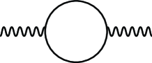
Figure 1: Two point function for $\tilde{a}$.

Other effects, such as the contributions from the electron-electron interactions, appear at higher orders in derivatives (and in the parity even sector only). Thus, to leading order we find the following effective Lagrangian  lopez-fradkin-98

$${\cal L}_{\rm eff}[\tilde{a},\tilde{b},\tilde{A}]=\frac{\hbar p}{4\pi}\epsilon^{\mu\nu\lambda}\tilde{a}_{\mu}\partial_{\nu}\tilde{a}_{\lambda}+\frac{\hbar}{2\pi}\epsilon^{\mu\nu\lambda}\tilde{a}_{\mu}\partial_{\nu}\tilde{b}_{\lambda}-\frac{2n\hbar}{4\pi}\epsilon^{\mu\nu\lambda}\tilde{b}_{\mu}\partial_{\nu}\tilde{b}_{\lambda}-\frac{1}{2\pi}\frac{e}{c}\epsilon^{\mu\nu\lambda}\tilde{A}_{\mu}\partial_{\nu}\tilde{b}_{\lambda}$$ (19)

where $\tilde{A}$ is a small fluctuation of the external electromagnetic field. Note that if we integrate out $\tilde{a}$, at leading order we get (up to boundary conditions)

$${\cal L}_{\rm eff}[\tilde{b}]=-(2n+\frac{1}{p})\frac{\hbar}{4\pi}\epsilon^{\mu\nu\lambda}\tilde{b}_{\mu}\partial_{\nu}\tilde{b}_{\lambda}+\ldots$$ (20)

The coefficient of ${\cal L}_{\rm eff}[\tilde{b}]$ is $\displaystyle{\nu^{-1}=2n+\frac{1}{p}}$. Thus $p=1$ corresponds to the Laughlin series. In particular, also for $p=1$, this is the form of the action that follows from hydrodynamic arguments wen-topo ; wen-zee-matrix ; wen-review ; frohlich-zee ; frohlich-kerler . It is straightforward to show  lopez-fradkin-91 that this theory leads to the correct value of the Hall conductivity

$$\sigma_{xy}=\frac{\nu}{2\pi}\;\frac{e^{2}}{\hbar c}$$ (21)

where

$$\frac{1}{\nu}=2n+\frac{1}{p}$$ (22)

This result is exact because it saturates a Ward identity, i. e. the $f$-sum rule, as discussed in Refs. lopez-fradkin-91 ; zhang .

The coefficient of the Chern-Simons action is known as the Chern-Simons level. General topological consistency arguments witten-cs ; hosotani show that if the theory is quantized on a closed manifold, the level of a Chern-Simons action must be quantized for the theory to be invariant under large gauge transformations. This requirement is met by the effective action of Eq. (19), which contains both the statistical and the hydrodynamic gauge fields, but not by either the effective action for the statistical field or the hydrodynamic field alone except for the Laughlin sequence, $p=1$. We will return to this issue in the context of the non-commutative theory in Section V.

IV.1 Trilinear Chern-Simons Couplings

Hence, to quadratic order in fluctuations and at long distances, one finds a commutative Abelian Chern-Simons gauge theory. We will investigate now the trilinear terms in this expansion.

We have seen that to quadratic order in $\tilde{a}$, and to lowest order in a gradient expansion, the effective action for a Laughlin FQH state and its Abelian generalizations is a (commutative) Abelian Chern-Simons theory. We will show now that the contributions to the effective action trilinear in $\tilde{a}$ make the effective theory non-commutative. The next correction, $S_{\rm eff}^{(3)}[\tilde{a}]$, is trilinear in the fields $\tilde{a}$, and it is shown in Fig. 2.

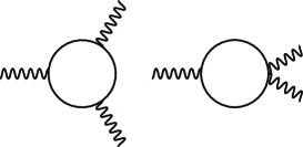
Figure 2: Diagrams contributing to the three point function for $\tilde{a}$.

The details of this calculation are given in the Appendix. In momentum space, we evaluate

$$S^{(3)}_{\rm eff}[\tilde{a}]=\frac{1}{3!}\int d^{3}P\ d^{3}Q\ d^{3}R\ \Pi^{\mu\nu\lambda}(P,Q,R)\tilde{a}_{\mu}(P)\tilde{a}_{\nu}(Q)\tilde{a}_{\lambda}(R)$$ (23)

It is difficult to evaluate the resulting sums and integrals entering in $\Pi^{\mu\nu\lambda}(P,Q,R)$ in closed form. They are given in the form of a series with frequency poles at integer multiples of the cyclotron frequency and with residues dictated by gauge invariance multiplied by factors involving Laguerre polynomials of the variable $P^{2}/2B_{\rm eff}$. The odd-parity terms of this tensor contain a phase factor of the form

$$e^{\displaystyle{-i\ell_{\rm eff}^{2}\;P\wedge Q}/2}$$ (24)

which we recognize as a Moyal phase. (To be more precise it is the Fourier transform of Eq. (10) with $\theta\to\ell_{\rm eff}^{2}$.) Notice that here $\ell_{\rm eff}^{2}=\hbar c/eB_{\rm eff}$ is the effective magnetic length, which is related to the magnetic length $\ell$ by

$$\ell_{\rm eff}^{2}=(2np+1)\ell^{2}=\frac{p}{\nu}\ell^{2}$$ (25)

To leading order in an expansion in momenta there is one component $\Pi^{012}$ which survives. We find, up to an energy-momentum conserving $\delta$-function

$$\Pi^{0[12]}(P,Q,R)=\frac{\hbar p}{2\pi}e^{-\displaystyle{i\ell_{\rm eff}^{2}\;P\wedge Q}/2}\;\;f(\vec{P}^{2},\vec{Q}^{2})$$ (26)

where $f(P^{2},Q^{2})$ is a regular function of the momenta $P$ and $Q$ and $f(0,0)=1$.

We are being selective in keeping the momentum dependent phase. To be fully consistent we should expand the exponential and group the momenta into higher derivative corrections. However, we claim that this phase is a Moyal phase indicative of the non-commutativity of this theory. This phase automatically accompanies all Feynman diagrams, and at least at one loop is the only odd parity contribution.

Thus, to the order of approximation we have kept, the effective Lagrangian for the statistical gauge fields $\tilde{a}$ is a non-commutative Chern-Simons gauge theory, of the form of Eq. (9), at level $p$:

$${\cal L}_{\rm eff}[\tilde{a}]=\frac{\hbar p}{4\pi}\epsilon^{\mu\nu\lambda}\left(\tilde{a}_{\mu}\partial_{\nu}\tilde{a}_{\lambda}-\frac{2i}{3}\tilde{a}_{\mu}\star\tilde{a}_{\nu}\star\tilde{a}_{\nu}\right)+\ldots$$ (27)

where $\star$ denotes a Moyal product of Eq. (24) with non-commutativity parameter $\theta_{a}=\ell_{\rm eff}^{2}$. Hence, to the present order of approximation, the trilinear terms just calculated turn the terms associated with the statistical gauge field $\tilde{a}$ in the effective action $S_{\rm eff}[a,b]$ of Eq. (19) into a non-commutative Chern-Simons gauge theory. The resulting effective action still satisfies the quantization condition of the level of its Chern-Simons terms.

However, there are a number of features of this result that seem to be wrong. Although this effective theory is non-commutative, the non-commutativity is associated with the statistical gauge field $\tilde{a}$ instead of the hydrodynamic gauge field $\tilde{b}$ as in Susskind’s action. In addition, the level of the non-commutative gauge theory is $p$ instead of the denominator of the filling factor as suggested by Ref. Suss . Likewise, the length scale of the non-commutativity is neither the average particle separation as in Susskind’s action nor the magnetic length $\ell$ as required by the magnetic current algebra, but instead the effective magnetic length $\ell_{\rm eff}$. We will show below, using the exact symmetries of the physical system, that at higher orders there must be corrections which conspire to yield the correct behavior for physical observables, such as the actual charge density and current.

These corrections are not hard to find. In fact the expansion of the fermion determinant leads to terms in the effective action for $\tilde{a}$ with more than three external legs. In particular the terms with an odd number of external legs have parity-odd pieces involving Moyal products as well as more derivatives. These terms cannot be neglected in the computation of the effective action for the hydrodynamic field $\tilde{b}$.

V The non-commutative duality

Let us now make contact with Susskind’s hydrodynamic effective theory. We will do that by integrating out the statistical gauge field $a$, and calculating an effective action for the hydrodynamic field $b$. Since the theory is now non-linear in $\tilde{a}$, we will do this in perturbation theory. Thus, we go back and consider the full non-commutative effective Lagrangian of Eq. (19):

$${\cal L}_{\rm eff}[\tilde{a},b] = \frac{\hbar p}{4\pi}\epsilon^{\mu\nu\lambda}\left\{\tilde{a}_{\mu}\partial_{\nu}\tilde{a}_{\lambda}-\frac{2i}{3}\tilde{a}_{\mu}\star\tilde{a}_{\nu}\star\tilde{a}_{\lambda}+\ldots\right\}+\frac{\hbar}{2\pi}\epsilon^{\mu\nu\lambda}\tilde{a}_{\mu}\partial_{\nu}b_{\lambda}-\frac{2n\hbar}{4\pi}\epsilon^{\mu\nu\lambda}b_{\mu}\partial_{\nu}b_{\lambda}$$

$$-\frac{e}{2\pi c}\epsilon^{\mu\nu\lambda}\tilde{A}_{\mu}\partial_{\nu}b_{\lambda}+\ldots$$

and integrate out $\tilde{a}$ perturbatively. Here the ellipses denote terms with more than three factors of $\tilde{a}$.

This expansion leads to an effective Lagrangian for the hydrodynamic field $b$, the dual theory, of the form

$${\cal L}_{\rm eff}[b]=-\frac{\hbar}{4\pi\nu}\epsilon^{\mu\nu\lambda}\left(b_{\mu}\partial_{\nu}b_{\lambda}-\frac{2i}{3}b_{\mu}\star b_{\nu}\star b_{\lambda}+\ldots\right)-\frac{e}{2\pi c}\epsilon^{\mu\nu\lambda}\tilde{A}_{\mu}\partial_{\nu}b_{\lambda}.$$ (28)

In order to write the effective action in this form, we have rescaled the $\star$-product. At the present level of approximation, the effective non-commutativity parameter appearing in eq. (28) is

$$\theta_{b}=\frac{1}{2np+1}\frac{\ell^{2}}{\nu}+\ldots$$ (29)

and the terms denoted by $\ldots$ are contributions to the trilinear term in $b$ originating from diagrams in the expansion on $\tilde{a}$ of the type shown in Fig. 3.

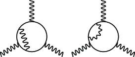
Figure 3: Two loop diagrams contributing to $\Pi^{\mu\nu\lambda}$. The internal wavy lines are propagators of the statistical gauge field $\tilde{a}$.

Such contributions, among other things, lead to finite renormalizations of the non-commutativity parameter.

For the particular case of the Laughlin sequence where $p=1$ and $\nu=1/(2n+1)$, we obtain an effective hydrodynamic theory of Susskind’s form at level $k=2n+1$ but with an effective non-commutativity parameter $\theta=\ell^{2}/\nu k$. In contrast, in Susskind’s theory Suss the non-commutativity parameter is $\theta=\ell^{2}/\nu=1/(2\pi\rho)$, i. e. the length scale of non-commutativity is the mean distance between electrons.

The effective hydrodynamic theory of Eq. (28) is dual to the theory described in terms of the statistical gauge field $a$. Under this transformation particles and fluxes are interchanged. This is just the particle-flux duality which underlies the physics of the fractional quantum Hall states. Hence, the effective theory of Eq. (28) is the non-commutative extension of the duality picture familiar from the commutative Chern-Simons theories of the fractional quantum Hall effect duality .

The effective action $S_{\rm eff}[\tilde{A}]$ for an electromagnetic perturbation $\tilde{A}$ can be computed by integrating out the hydrodynamic field $b$. To lowest order we find

$$S_{\rm eff}=\frac{\nu e^{2}}{4\pi\hbar c^{2}}\int d^{3}x\;\epsilon^{\mu\nu\lambda}\left(\tilde{A}_{\mu}\partial_{\nu}\tilde{A}_{\lambda}-\frac{2i}{3}\;\frac{e}{\hbar c}\tilde{A}_{\mu}\star\tilde{A}_{\nu}\star\tilde{A}_{\lambda}+\ldots\right)$$ (30)

with a non-commutativity parameter which is now

$$\theta_{A}=\displaystyle{\frac{\ell^{2}}{2np+1}+\ldots}$$ (31)

This result implies that the Hall conductivity is $\sigma_{xy}=\nu e^{2}/h$, which is correct, but it predicts a non-commutativity parameter $\theta$ which is not equal to $\ell^{2}$. Below we will present an argument, essentially a Ward identity, which implies that for a translationally invariant system in a magnetic field the non-commutativity parameter should be exactly equal to $\ell^{2}$ without any renormalization. This result also implies that the non-commutativity parameter of the hydrodynamic theory must be exactly equal to $\ell^{2}/\nu=1/(2\pi\rho)$ as in Susskind’s theory. Hence, the non-linear terms in the effective action for the statistical field $\tilde{a}$ must lead to perturbative contributions in the hydrodynamic theory whose total net effect is a finite renormalization of its non-commutativity parameter to the correct value $\ell^{2}/\nu$. In contrast the level of the Chern-Simons action cannot be renormalized as it is protected by topological invariance.

V.1 Magnetic Ward Identity

In the previous sections we showed that the Moyal phase appearing in Eq. (26) indicates that the effective action for $\tilde{a}$ should be considered non-commutative. However this result led to a number of inconsistencies which we will discuss here. As we noted above, the Moyal phase appearing in Eq.  (26) is controlled by $B_{\rm eff}$, which sets the length scale relevant to the perturbation theory about the mean field state. However, as we noted above, $B_{\rm eff}$ is not a physical scale.

The mean field theory that we used here, usually called the average field approximation, is known to break a number of symmetries of the physical electron gas which must be preserved exactly. Let us reexamine what we have done. We first attached $2n$ flux quanta to each electron. This procedure does not change anything and it does not break any symmetry. However, at the mean field level, there are significant changes in the Hilbert space: the system behaves like a system of composite fermions filling up an integer number $p$ of Landau levels of the partially screened magnetic field $B_{\rm eff}$. In particular these effective levels are mixtures of the original Landau levels. This is the physics of the (unprojected) Jain wave functions jain . If taken literally, this mean field theory makes a number of wrong predictions. For instance it implies that the bosonic bound state with the leading residue, i. e. a residue which vanishes like $\sim q^{2}$ as $\vec{q}\to 0$ as required by gauge invariance, has an energy gap at the effective cyclotron frequency $\omega_{\rm eff}=\omega/(2np+1)$. As it is well known, this result violates Kohn’s theorem kohn , which states that in a translationally invariant system this gap must be at the exact cyclotron frequency $\omega_{c}=eB/mc$, without any mass renormalization. Kohn’s theorem follows from the fact that the system as a whole must obey the magnetic algebra of the full magnetic field $B$. (A similar approximation also leads to a spurious zero-field Hall effect in theories of anyon superfluidity cwwh .) Similarly, the excitation spectrum predicted by this mean field theory is wrong, since it predicts that the excitations of this state are composite fermions instead of particles with fractional charge and fractional statistics. The problem with the length scale in the Moyal phase has the same origin.

The solution to these problems is well known. At the level of wave functions, the correct physical behavior is recovered only after the states are projected onto the lowest Landau level jain . In the context of the Chern-Simons theories, which deal with electrons as point particles and are not projected onto the lowest Landau level, the solution to these problems is also well understood. It has been shown in Refs.  lopez-fradkin-91 ; lopez-fradkin-93 ; zhang , that unlike other mean field theories, for fractional quantum Hall states, quantum fluctuations even at the Gaussian level, restore some of the symmetries broken by the the mean field state. Physically this happens since, due to the Gauss Law constraint of the Chern-Simons theory, a local density fluctuation is equivalent to a local flux fluctuation. In particular, the leading quantum corrections, described by the Gaussian commutative effective action, yield upon integrating out the gauge fields $a$ and $b$, the correct electromagnetic polarization tensor which saturates the $f$-sum rule in the $\vec{q}\to 0$ regime and thus it is exact in this limit lopez-fradkin-91 ; lopez-fradkin-98 ; lopez-fradkin-93 . Hence, in the uniform limit this theory predicts, for the Jain states with filling factor $\nu=p/(2np+1)$, a Hall conductivity equal to $\sigma_{xy}=\frac{\nu}{2\pi}\frac{e^{2}}{\hbar}$, a cyclotron mode with frequency $\omega_{c}$ and residue $\sim\vec{q}^{\;2}$, a spectrum of quasiholes carrying charge $e/(2np+1)$ and fractional statistics $\pi/(2np+1)$, and, for a surface of genus $g$, a ground state degeneracy of $(2np+1)^{g}$. Thus the (Gaussian) commutative Chern-Simons effective action of Eq. (19) yields a complete description of the universal long-distance data of fractional quantum Hall states (for a recent discussion see Ref. lopez-fradkin-98 ). (This is no longer the case when the gap collapses as in the limiting states $\nu=1/2n$, which are compressible states of the 2DEG hlr .)

Let us see what this line of analysis implies for the non-commutative effective theory of Eq. (19) and Eq. (27). We noted before that in the $\vec{q}\to 0$ limit the Gaussian theory is exact. However, in this regime the theory is commutative. Although at shorter distances, the physics of the 2DEG is strongly non-universal, we showed above that in the odd-parity sector, the theory becomes non-commutative. However, the length scale of the non-commutativity is $\ell_{\rm eff}$ which is not a physical length scale. This inconsistency has exactly the same origin as the violation of the global magnetic symmetry. As before, this inconsistency is also resolved by quantum corrections to the mean field state.

To understand this problem, let us look first at the actual electromagnetic currents $J_{\mu}$ in the system. (As usual, this is a $3$-vector formed by the physical charge density fluctuation and the two components of the charge current.) These currents are obtained as from the effective action for the external electromagnetic gauge field $S_{\rm eff}[\tilde{A}]=-\log Z[\tilde{A}_{\mu}]$, where $Z[\tilde{A}]$ is the partition function of the full 2DEG and $\tilde{A}$ is a weak electromagnetic perturbation. In 1992, Iso, Karabali and Sakita sakita , and independently Martinez and Stone stone , showed that the electromagnetic currents and charge densities for a 2DEG in a large magnetic field $B$, in an incompressible state with filling factor $\nu$, obey a $W_{\infty}$ algebra, which is a local extension of the global magnetic algebra of finite translation operators in a magnetic field. Let $\hat{\rho}(x,y)$ be the charge density operator projected on the Lowest Landau level, and $\hat{\rho}(p,q)$ be its Fourier transform

$$\hat{\rho}(p,q)=\int dxdy\;\hat{\rho}(x,y)\;e^{\displaystyle{i(px+qy)/\hbar}}$$ (32)

These authors girvin-jach ; sakita ; stone showed that the projected density operators obey the algebra

$$\left[\hat{\rho}(p,q),\hat{\rho}(p^{\prime},q^{\prime})\right]=-2i\sin\left(\ell^{2}(pq^{\prime}-p^{\prime}q)/2\right)\;e^{\ell^{2}(pp^{\prime}+qq^{\prime})/2}\hat{\rho}(p+p^{\prime},q+q^{\prime})$$ (33)

In the holomorphic basis

$$\hat{\rho}_{mn}=\int dxdy\;\hat{\rho}(x,y)\;z^{m}\bar{z}^{n}$$ (34)

the algebra becomes

$$\left[\hat{\rho}_{mn},\hat{\rho}_{kl}\right]=\sum_{j=1}^{{\rm min}(n,k)}\frac{(-1)^{j}}{j!}\frac{n!k!}{(n-j)!(k-j)!}\hat{\rho}_{m+k-j,n+l-j}-(n\leftrightarrow l)(m\leftrightarrow k)$$ (35)

Hence, the algebra of the charge density operators  girvin-jach ; sakita , as well as of the current density operators as shown in Ref. stone , contains explicitly a Moyal product controlled by the magnetic length scale $\ell$ of the full magnetic field $B$. This is a very general result which follows from the incompressibility of the system and from the properties of the quantum states in a magnetic field.

This result poses important constraints, which can be regarded as Ward identities, on the values of the parameters of the effective action $S_{\rm eff}[\tilde{A}]$ of an external electromagnetic field in an incompressible quantum Hall state. In addition to the condition of gauge invariance, which follows from current conservation, these results require that for a fractional quantum Hall state at filling factor $\nu$, the effective action $S_{\rm eff}[\tilde{A}]$ must have the form of a non-commutative Chern-Simons action whose level is $\nu$ (in units of $e^{2}/\hbar$) and whose non-commutativity parameter $\theta=\ell^{2}=\hbar c/eB$, where $B$ is the full magnetic field. As we saw above, this requirement in turn implies that the non-commutativity scale for the hydrodynamic field is $1/(2\pi\rho)$, where $\rho$ is the average areal density. Therefore, we conclude that the higher orders in perturbation theory, among other things, must necessarily renormalize the non-commutativity parameter of the hydrodynamic field to this exact value.

VI Conclusions

In this paper we have used the notion of flux attachment to derive Susskind’s non-commutative hydrodynamic action for the fractional quantum Hall effect. We have presented two mutually dual effective theories, which are non-commutative extensions of the familiar (commutative) Chern-Simons descriptions of the FQHE. We have used this duality to show that while the hydrodynamic effective action must have a non-commutative parameter controlled by the average particle distance (as in Susskind’s action), the effective action of the electromagnetic field must have a non-commutative parameter controlled only by the magnetic length. We have also shown that while mean-field-like approximations do lead to effective actions with the correct form of a non-commutative Chern-Simons theory, the non-commutativity parameter is not correct at lowest order and must acquire corrections in order to satisfy the constraints imposed by the global magnetic algebra, and its local (Moyal) extension. This is in marked contrast with the Hall conductivity which is already correct at the level of the Gaussian theory.

We would like to comment on the validity and usefulness of these non-commutative effective theories. Clearly the commutative abelian Chern-Simons theory gives a faithful description of the universal data encoded in fractional quantum Hall fluids: the Hall conductivity, the fractional charge and statistics of the excitations and the global topological degeneracy of their ground states. The non-commutative theory describes the local extension of the global magnetic algebra, i. e. the $W_{\infty}$ algebra of the local currents and densities of incompressible charged two-dimensional fluids in large magnetic fields. In fact, as argued by Susskind, non-commutative Chern-Simons theory is a description of the area-preserving diffeomorphisms of these incompressible fluids. Hence, in a sense, except for the universal quantum numbers they encode, the information contained in these effective theories is essentially kinematic in nature. Indeed, there is much dynamics taking place at the scale of the magnetic (and Coulomb) lengths, such as the energetics of the excitations, which is not described by these effective theories. Although in a formal sense this is an inconsistency, what matters here is that the non-commutative terms included are the only contributions at these length scales which are odd under parity and time-reversal. Obviously a full description of the physics requires the (strongly non-universal) microscopic physics which controls the energetics of these states.

These considerations are particularly important for applications of these ideas to non-uniform ground states such as Wigner crystals, quantum Hall smectic and nematic states (for recent work see Refs. fogler ; chalker ; FK ; bert ; barci ; fogler2 ; RD ). Recent work on these interesting phases of the two-dimensional electron gas has revealed that magnetic symmetry plays a crucial role in low-energy dynamics of these states. Interestingly, recent work on non-commutative field theories has suggested that their phase diagrams involve analogs of these phases gubser-sondhi . It remains an important and open problem to understand the implications and restrictions imposed by the non-commutative structure on the phase transitions between these states sinova ; moore .

VII Acknowledgments

Discussions with Moshe Rozali and Michael Stone are gratefully acknowledged. Work supported in part by U. S. Department of Energy, grant DE-FG02-91ER40677 (RL), and by the National Science Foundation through the grant DMR-01-32990 (EF). VJ has been supported by a GAANN fellowship from the U.S. Department of Education, grant 1533616.

Appendix A

In this appendix, we give details of the perturbative computations. For a detailed discussion of the physics behind this theory, see Ref. lopez-fradkin-91 . We borrow their notation, and pick up the discussion at an appropriate point. Within this appendix, we have set $e=\hbar=c=1$, and thus $B_{\rm eff}=1/\ell_{\rm eff}^{2}$. The Feynman rules are obtained from the Lagrangian density for non-relativistic fermions in a magnetic field:

$${\cal L}=\psi^{\dagger}L\psi-{a}_{0}\psi^{\dagger}\psi+\frac{i}{2M}{a}_{j}\left[(D_{j}^{\dagger}\psi^{\dagger})\psi-\psi^{\dagger}D_{j}\psi\right]+\frac{1}{2M}\vec{a}^{2}\psi^{\dagger}\psi$$ (36)

where

$$D=\partial+iA,\ \ \ \ \ D^{\dagger}=\partial-iA$$ (37)

$$L=i\partial_{0}-A_{0}+\mu+(1/2m)\vec{D}^{2}$$ (38)

The propagator is written $\langle\psi(x_{1})\psi^{\dagger}(x_{2})\rangle=iG(x_{1},x_{2}).$ It is convenient for this calculation to rescale spatial coordinates $\vec{u}_{i}=\sqrt{B_{\rm eff}}\ \vec{x}_{i}$ and similarly rescale momenta $\vec{P}_{i}\to\vec{P}_{i}/\sqrt{B_{\rm eff}}$. We then have

$$iG(u,v)=\int\frac{dk}{2\pi}\ S_{x^{0},y^{0},m}\varphi_{m,k}(\vec{u})\varphi^{*}_{m,k}(\vec{v})$$ (39)

where for brevity we have written the summation symbol

$$S_{x^{0},y^{0},m}=\left(\theta(x^{0}-y^{0})\sum_{m=p}^{\infty}-\theta(y^{0}-x^{0})\sum_{m=0}^{p-1}\right)e^{-i\omega_{m}(x^{0}-y^{0})}$$ (40)

and

$$\varphi_{m,k}(\vec{u})={\cal N}_{m}e^{iku_{x}}\ e^{-(u_{y}-k)^{2}/2}\ H_{m}(u_{y}-k)$$ (41)

with normalization ${\cal N}_{m}=(2^{m}m!\sqrt{\pi})^{-1/2}$. We choose a gauge such that

$$\frac{iD^{(x)}_{x}}{M} = \alpha\left(i\frac{\partial}{\partial u_{x}}+u_{y}\right)\equiv d_{x}^{(u)}$$ (42)

$$\frac{iD^{(x)}_{y}}{M} = i\alpha\frac{\partial}{\partial u_{y}}\equiv d_{y}^{(u)}.$$ (43)

where $\alpha=\sqrt{B_{\rm eff}}/M$. These derivatives have the effect of shifting the indices of the Landau functions:

$$d_{a}^{(u_{1})}iG(u_{1},u_{2})=\alpha\int\frac{dk}{2\pi}\ S_{x^{0},y^{0},m}\sum_{J}c_{m,a}^{(J)}\varphi_{m+J,k}(\vec{u}_{1})\varphi^{*}_{m,k}(\vec{u}_{2})$$

$$d_{a}^{(u_{1})\dagger}iG(u_{3},u_{1})=\alpha\int\frac{dk}{2\pi}\ S_{x^{0},y^{0},m}\varphi_{m,k}(\vec{u}_{3})\sum_{\tilde{J}}\tilde{c}_{m,a}^{(\tilde{J})}\varphi^{*}_{m+\tilde{J},k}(\vec{u}_{1})$$

where we have introduced constants $c$ and $\tilde{c}$, whose non-zero components are:

$$c_{m,x}^{(1)} =\sqrt{\frac{m+1}{2}},\ \ \ \ \ \ \ c_{m,y}^{(1)}=-i\sqrt{\frac{m+1}{2}}$$ (44)

$$c_{m,x}^{(-1)} =\sqrt{\frac{m}{2}},\ \ \ \ \ \ \ c_{m,y}^{(-1)}=+i\sqrt{\frac{m}{2}}$$ (45)

$$\tilde{c}_{m,x}^{(1)} =\sqrt{\frac{m+1}{2}},\ \ \ \ \ \ \ \tilde{c}_{m,y}^{(1)}=+i\sqrt{\frac{m+1}{2}}$$ (46)

$$\tilde{c}_{m,x}^{(-1)} =\sqrt{\frac{m}{2}},\ \ \ \ \ \ \ \tilde{c}_{m,y}^{(-1)}=-i\sqrt{\frac{m}{2}}$$ (47)

In the three-point Feynman diagrams (Figs. 2), for each spatial component of a gauge field that appears at an external leg, there is a spatial derivative of the form given above acting on the fermion lines. If we sum over all such possibilities, the net effect on a vertex is to replace its Landau functions by a factor

$$\sum_{\tilde{J}_{1},J_{2}}C_{\tilde{J}_{1},J_{2}}(m_{1},m_{2};\mu)\varphi^{*}_{m_{1}+\tilde{J}_{1},k_{1}}(\vec{u}_{2})\varphi_{m_{2}+J_{2},k_{2}}(\vec{u}_{2}).$$ (48)

It is not difficult to show that

$$C_{\tilde{J}_{1},J_{2}}(m_{1},m_{2};0) = \delta_{\tilde{J}_{1},0}\delta_{J_{2},0}$$ (49)

$$C_{\tilde{J}_{1},J_{2}}(m_{1},m_{2};a) = \frac{\alpha}{2}\left(c_{m_{2},a}^{(J_{2})}\delta_{\tilde{J}_{1},0}+\tilde{c}_{m_{1},a}^{(\tilde{J}_{1})}\delta_{J_{2},0}\right),\ \ \ \ \ a=x,y.$$ (50)

$C$ is essentially the “Fourier transformed” three point vertex of $\psi^{\dagger}a_{\mu}\psi$.

We write the correction to the effective action as

$$\delta S_{eff}=\frac{1}{3!}\int d^{3}x_{1}d^{3}x_{2}d^{3}x_{3}\ a_{\mu_{1}}(x_{1})a_{\mu_{2}}(x_{2})a_{\mu_{3}}(x_{3})\Pi^{\mu_{1}\mu_{2}\mu_{3}}(x_{1},x_{2},x_{3})$$ (51)

where $\Pi$ is

$$\int\sum_{\vec{J},\vec{\tilde{J}}}\prod_{j=1}^{3}\left[\frac{dk_{j}}{2\pi}S_{x_{j}^{0},x_{j+1}^{0},m_{j}}C_{\tilde{J}_{j},J_{j+1}}(m_{j},m_{j+1};\mu_{j+1})\varphi_{m_{j}+J_{j},k_{j}}(\vec{u}_{j})\varphi^{*}_{m_{j-1}+\tilde{J}_{j-1},k_{j-1}}(\vec{u}_{j})\right]$$ (52)

(Note: actually, this is just one of the two Feynman diagrams. The other can contribute only to $\Pi^{aa\mu}$.) To proceed, we Fourier transform the CS fields

$$a_{\mu}(x)=\int dP^{0}d^{2}Pa_{\mu}(P)e^{iP^{0}x^{0}}e^{-i\vec{P}\cdot\vec{u}}$$ (53)

Note that $\vec{P}$ here is the rescaled momentum.

It is then a simple matter to perform the integrals over the time coordinates; the net effect is that the sums and $\theta$-functions are replaced by $2\pi\delta(P_{0}+Q_{0}+R_{0})$ times

$$T=\frac{\left[\sum_{m_{1}=p}^{\infty}\sum_{m_{2}=p}^{\infty}\sum_{m_{3}=0}^{p-1}-\sum_{m_{1}=0}^{p-1}\sum_{m_{2}=0}^{p-1}\sum_{m_{3}=p}^{\infty}\right]}{(\omega_{m_{3}}-\omega_{m_{1}}+P_{0})(\omega_{m_{3}}-\omega_{m_{2}}-R_{0})}+{\rm cyclic}$$ (54)

where we cycle simultaneously on $P_{0},Q_{0},R_{0}$ and $m_{1},m_{2},m_{3}$.

Next, we can do the spatial integrals, using the orthogonality for the $\varphi$’s

$$\int d^{2}u\ \varphi_{m,k}(\vec{u})\varphi^{*}_{m^{\prime},k^{\prime}}(\vec{u})e^{-i\vec{P}\cdot\vec{u}}=2\pi\delta(k-k^{\prime}-P_{x})e^{-\vec{P}^{2}/4}e^{-iP_{y}(k+k^{\prime})/2}{\cal L}_{m,m^{\prime}}(\vec{P})$$ (55)

where

$${\cal L}_{m,m^{\prime}}(\vec{P}) = \left(\theta(m-m^{\prime})\sqrt{\frac{m^{\prime}!}{m!}}\left(-{\cal P}\right)^{m-m^{\prime}}L_{m^{\prime}}^{m-m^{\prime}}(|{\cal P}|^{2})\right.$$ (57)

$$+\left.\theta(m^{\prime}-m)\sqrt{\frac{m!}{m^{\prime}!}}\left({\cal P}^{*}\right)^{m^{\prime}-m}L_{m}^{m^{\prime}-m}(|{\cal P}|^{2})\right)$$

where we have defined ${\cal P}=(P_{x}+iP_{y})/\sqrt{2}$.

Thus we find

$$\int\prod_{j=1}^{3}\left[\frac{dk_{j}}{2\pi}\ 2\pi\delta(k_{j}-k_{j-1}-P_{j,x})e^{-\vec{P}_{j}^{2}/4}e^{-iP_{j,y}(k_{j}+k_{j-1})/2}\right]\times$$

$$T\left\{\sum_{\vec{J},\vec{\tilde{J}}}\prod_{j=1}^{3}C_{\tilde{J}_{j-1},J_{j}}(m_{j-1},m_{j};\mu_{j}){\cal L}_{m_{j}+J_{j},m_{j-1}+\tilde{J}_{j-1}}(\vec{P}_{j})\right\}$$ (58)

Performing the $k_{j}$-integrations, we find

$$\frac{1}{2\pi}e^{-i(P_{1,x}P_{2,y}-P_{1,y}P_{2,x})/2}T\left\{\sum_{\vec{J},\vec{\tilde{J}}}\prod_{j=1}^{3}e^{-\vec{P}^{2}_{j}/4}C_{\tilde{J}_{j-1},J_{j}}(m_{j-1},m_{j};\mu_{j}){\cal L}_{m_{j}+J_{j},m_{j-1}+\tilde{J}_{j-1}}(\vec{P}_{j})\right\}$$ (59)

(We have dropped an overall energy-momentum conserving $\delta$-function.) We note that this result carries an overall Moyal phase, times a complicated function of energies and momenta.

To proceed further, we need to evaluate the rather complicated sums in eq. (59). We will do so by expanding in energies and momenta (keeping the overall Moyal phase intact). We find that there is a non-zero contribution to the parity odd polarization

$$\Pi^{0[12]}(P_{1},P_{2},P_{3})=\frac{p}{2\pi}e^{\displaystyle{-i\ell_{\rm eff}^{2}\;P_{1}\wedge P_{2}/2}}\;\;f(P_{1}^{2},P_{2}^{2})$$ (60)

where $f(P^{2},Q^{2})$ is a regular function of the momenta $P$ and $Q$ and $f(0,0)=1$. Contributions to other polarizations of $\Pi$ are also calculable, but are of no relevance to the discussions of this paper.

References

- (1) R. B. Laughlin, Phys. Rev. Lett. 50, 1395 (1983).
- (2) F. D. M. Haldane, Phys. Rev. Lett. 51, 605 (1983).
- (3) B. I. Halperin, Phys. Rev. Lett. 52, 1583 (1984).
- (4) J. K. Jain, Phys. Rev. Lett. 63, 199 (1989); Phys. Rev. B 40, 8079 (1989); Adv. Phys. 41, 105 (1992).
- (5) X. G. Wen and Q. Niu, Phys. Rev. B 41, 9377 (1990)
- (6) X. G. Wen, Phys. Rev. B 40, 7387 (1989).
- (7) S. C. Zhang, T. H. Hansson and S. Kivelson, Phys. Rev. Lett. 62, 82 (1989).
- (8) A. Lopez and E. Fradkin, Phys. Rev. B 44, 5246 (1991).
- (9) S. C. Zhang, Int. J. Mod. Phys. B 6, 25 (1992).
- (10) B. Blok and X. G. Wen, Phys. Rev. B 43, 8337 (1991).
- (11) X. G. Wen, Adv. Phys. 44, 405 (1995).
- (12) X. G. Wen and A. Zee, Phys. Rev. B 46, 2290 (1992).
- (13) J. Fröhlich and A. Zee, Nucl. Phys. B 364, 517 (1991).
- (14) J. Fröhlich and T. Kerler, Nucl. Phys. B 354, 369 (1991).
- (15) S. Bahcall and L. Susskind, Int. J. Mod. Phys. B 5, 2735 (1991).
- (16) L. Susskind, The quantum Hall fluid and non-commutative Chern Simons theory, hep-th/0101029.
- (17) S. M. Girvin and T. Jach, Phys. Rev. B 29, 5617 (1984).
- (18) S. Iso, D. Karabali, and B. Sakita, Phys. Lett. B 296, 143 (1992).
- (19) J. Martinez and M. Stone, Int. J. Mod. Phys. B 7, 4389 (1993).
- (20) A. Capelli, C.A. Trugenberger, and G.R. Zemba, Nucl. Phys. B 396, 465 (1993).
- (21) S. M. Girvin, A. H. MacDonald and P. Platzman, Phys. Rev. B 33, 2481 (1986).
- (22) C. D. Fosco and A. López, Aspects of non-commutative descriptions of planar systems in high magnetic fields, hep-th/0106136.
- (23) E. Fradkin, C. Nayak, A. Tsvelik and F. Wilczek, Nucl. Phys. B 516 [FS], 704 (1998).
- (24) A. Lopez and E. Fradkin, Phys. Rev. B 59, 15323 (1999).
- (25) F. Wilczek and A. Zee, Phys. Rev. Lett. 51, 2250 (1983).
- (26) Y. S. Wu and A. Zee, Phys. Lett. 174 B, 325 (1984).
- (27) B. I. Halperin, P. A. Lee and N. Read, Phys. Rev. B 47, 7312 (1993).
- (28) E. Witten, Comm. Math. Phys. 121, 351 (1989).
- (29) Y. Hosotani, Phys. Rev. Lett. 62, 2785 (1989).
- (30) The concept of duality used here is essentially electro-magnetic duality. See D-H. Lee and M. P. A. Fisher, Phys. Rev. Lett. 63, 903 (1989); S. A. Kivelson, D-H. Lee and S-C. Zhang, Phys. Rev. B 46, 2223 (1992); C. A. Lütken and G. G. Ross, Phys. Rev. B 48, 2500 (1993); E. Fradkin and S. A. Kivelson, Nucl. Phys. B 474, 543 (1996).
- (31) Walter Kohn, Phys. Rev. 123, 1242 (1961).
- (32) Y.H.Chen, F.Wilczek, E.Witten and B.I.Halperin, Int. J. Mod. Phys. B 3, 1001 (1989).
- (33) A. Lopez and E. Fradkin, Phys. Rev. B 47, 7080 (1993).
- (34) A. A. Koulakov, M. M. Fogler, and B. I. Shklovskii, Phys. Rev. Lett. 76, 499 (1996).
- (35) R. Moessner and T. J. Chalker, Phys. Rev. B 54, 5006 (1996).
- (36) Eduardo Fradkin and Steven A. Kivelson, Phys. Rev. B 59, 8065 (1999).
- (37) Anna Lopatnikova, Steven H. Simon, Bertrand I. Halperin and Xiao-Gang Wen, Phys. Rev. B 64, 155301 (2001), cond-mat/0105079.
- (38) D. Barci, E. Fradkin, S. A. Kivelson and V. Oganesyan, to be published in Phys. Rev. B (2002), cond-mat/0105448.
- (39) M. Fogler, cond-mat/0107306.
- (40) L. Radzihovsky and A. Dorsey, Phys. Rev. Lett. 88, 216802 (2002), cond-mat/0110083.
- (41) S. Gubser and S. L. Sondhi, Nucl. Phys. B 605, 395-424 (2001).
- (42) J. Sinova, V. Meden, S. M. Girvin, Phys. Rev. B 62, 2008 (2000).
- (43) J. Moore, A. Zee and J. Sinova, Phys. Rev. Lett. 87, 046801/1-4 (2001), cond-mat/0012341.