The Dynamic Phase Transition for Decoding Algorithms

Abstract

The state-of-the-art error correcting codes are based on large random constructions (random graphs, random permutations, …) and are decoded by linear-time iterative algorithms. Because of these features, they are remarkable examples of diluted mean-field spin glasses, both from the static and from the dynamic points of view. We analyze the behavior of decoding algorithms using the mapping onto statistical-physics models. This allows to understand the intrinsic (i.e. algorithm independent) features of this behavior.

LPTENS 02/31

1 Introduction

Recently there has been some interest in studying “complexity phase transitions”, i.e. abrupt changes in the computational complexity of hard combinatorial problems as some control parameter is varied [1]. These phenomena are thought to be somehow related to the physics of glassy systems, where the physical dynamics experiences a dramatic slowing down as the temperature is lowered [2].

Complexity is a central issue also in coding theory [3, 4]. Coding theory [5, 7, 6] deals with the problem of communicating information reliably through an unreliable channel of communication. This task is accomplished by making use of error correcting codes. In 1948 Shannon [8] proved that almost any error correcting code allows to communicate without errors, as long as the rate of transmitted information is kept below the capacity of the channel. However decoding is an intractable problem for almost any code. Coding theory is therefore a rich source of interesting computational problems.

On the other hand it is known that error correcting codes can be mapped onto disordered spin models [9, 10, 11, 12, 13]. Remarkably there has recently been a revolution in coding theory which has brought to the invention of new and very powerful codes based on random constructions: turbo codes [14], low density parity check codes (LDPCC) [15, 16], repetition accumulated codes [17], etc. As a matter of fact the equivalent spin models have been intensively studied in the last few years. These are diluted spin glasses, i.e. spin glasses on random (hyper)graphs [18, 19, 20, 21].

The new codes are decoded by using approximate iterative algorithms, which are closely related to the TAP-cavity approach to mean field spin glasses [22, 23]. We think therefore that a close investigation of these systems from a statistical physics point of view, having in mind complexity (i.e. dynamical) issues, can be of great theoretical interest.

Figure 1: A schematic description of how error correcting codes work.

Let us briefly recall the general setting of coding theory [5] in order to fix a few notations (cf. Fig. 1 for a pictorial description). A source of information produces a stream of symbols. Let us assume, for instance, that the source produces unbiased random bits. The stream is partitioned into blocks of length $N_{\rm block}$. Each of the possible $2^{N_{\rm block}}$ blocks is mapped to a codeword (i.e. a sequence of bits) of length $N>N_{\rm block}$ by the encoder and transmitted through the channel. An error correcting code is therefore defined either as a mapping $\{{\tt 0},{\tt 1}\}^{N_{\rm block}}\to\{{\tt 0},{\tt 1}\}^{N}$, or as a list of $2^{N_{\rm block}}$ codewords. The rate of the code is defined as $R=N_{\rm block}/N$.

Let us denote the transmitted codeword by $\underline{{\tt x}}^{\rm in}=[{\tt x}^{\rm in}_{1},\dots,{\tt x}^{\rm in}_{N}]^{\tt T}$. Due to the noise, a different sequence of symbols $\underline{{\tt x}}^{\rm out}=[{\tt x}^{\rm out}_{1},\dots,{\tt x}^{\rm out}_{N}]^{\tt T}$ is received. The decoding problem is to infer $\underline{{\tt x}}^{\rm in}$ given $\underline{{\tt x}}^{\rm out}$, the definition of the code, and the properties of the noisy channel.

It is useful to summarize the general picture which emerges from our work. We shall focus on Gallager codes (both regular and irregular). The optimal decoding strategy (maximum-likelihood decoding) is able to recover the transmitted message below some noise threshold: $p<p_{c}$. Iterative, linear time, algorithms get stuck (in general) at a lower noise level, and are successful only for $p<p_{d}({\rm alg.})$, with $p_{d}({\rm alg.})\leq p_{c}$. In general the “dynamical” threshold $p_{d}({\rm alg.})$ depends upon the details of the algorithm. However, it seems to be always smaller than some universal (although code-dependent) value $p_{d}$. Moreover, some “optimal” linear-time algorithms are successful up to $p_{d}$ (i.e. $p_{d}({\rm alg.})=p_{d}$). The universal threshold $p_{d}$ coincides with the dynamical transition [2] of the corresponding spin model.

The plan of the paper is the following. In Section 2 we introduce low density parity check codes (LDPCC), focusing on Gallager’s ensembles, and we describe message passing decoding algorithms. We briefly recall the connection between this algorithms and the TAP-cavity equations for mean-field spin glasses. In Sec. 3 we define a spin model which describes the decoding problem, and introduce the replica formalism. In Sec. 4 we analyze this model for a particular choice of the noisy channel (the binary erasure channel). In this case calculations can be fully explicit and the results are particularly clear. Then, in Sec. 5, we address the general case. Finally we draw our conclusions in Sec. 6. The Appendices collect some details of our computations.

2 Error correcting codes, decoding algorithms and the cavity equations

This Section introduces the reader to some basic terminology in coding theory. In the first part we define some ensembles of codes, namely regular and irregular LDPCC. In the second one we describe a class of iterative decoding algorithms. These algorithms have a very clear physical interpretation, which we briefly recall. Finally we explain how these algorithms are analyzed in the coding theory community. This Section does not contain any original result. The interested reader may consult Refs. [34, 15, 7, 23] for further details.

2.1 Encoding $\dots$

Low density parity check codes are defined by assigning a binary $N\times M$ matrix ${\mathbb{H}}=\{H_{ij}\}$, with $H_{ij}\in\{0,1\}$. All the codewords are required to satisfy the constraint

$${\mathbb{H}}\,\underline{{\tt x}}=0\;\;\;\;({\rm mod}\;\;\;2)\,.$$ (2.1)

The matrix ${\mathbb{H}}$ is called the parity check matrix and the $M$ equations summarized in Eq. (2.1) are the parity check equations (or, for short, parity checks). If the matrix ${\mathbb{H}}$ has rank $M$ (this is usually the case), the rate is $R=1-M/N$.

There exists a nice graphic representation of Eq. (2.1) which is often used in the coding theory community: the Tanner graph representation [35, 36]. One constructs a bipartite graph by associating a left-hand node to each one of the $N$ variables, and a right-hand node to each one of the $M$ parity checks. An edge is drawn between the variable node $i$ and the parity check node $\alpha$ if and only if the variable ${\tt x}_{i}$ appears with a non-zero coefficient in the parity check equation $\alpha$.

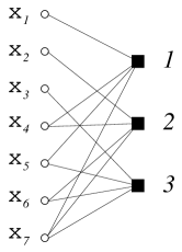
Figure 2: The Tanner graph for the ${\cal H}_{2}(3)$ Hamming code.

Let us for instance consider the celebrated ${\cal H}_{2}(3)$ Hamming code (one of the first examples in any book on coding theory). In this case we have $N=7$, $M=3$ and

$${\mathbb{H}}=\left[\begin{array}[]{ccccccc}1&0&0&1&1&0&1\\ 0&1&0&1&0&1&1\\ 0&0&1&0&1&1&1\\ \end{array}\right]\,.$$ (2.5)

This code has $2^{4}=16$ codewords $\underline{{\tt x}}^{(\alpha)}=[{\tt x}^{(\alpha)}_{1},\dots,{\tt x}^{(\alpha)}_{7}]^{\tt T}$, with $\alpha\in\{1,\dots,16\}$. They are the solutions of the three parity check equations: ${\tt x}_{1}+{\tt x}_{4}+{\tt x}_{5}+{\tt x}_{7}=0$; ${\tt x}_{2}+{\tt x}_{4}+{\tt x}_{6}+{\tt x}_{7}=0$; ${\tt x}_{3}+{\tt x}_{5}+{\tt x}_{6}+{\tt x}_{7}=0$ $({\rm mod}2)$. The corresponding Tanner graph is drawn in Fig. 2.

In general one considers ensembles of codes, by defining a random construction of the parity check matrix. One of the simplest ensembles is given by regular $(k,l)$ Gallager codes. In this case one chooses the matrix ${\mathbb{H}}$ randomly among all the $N\times M$ matrices having $k$ non-zero entries per row, and $l$ per column. The Tanner graph is therefore a random bipartite graph with fixed degrees $k$ and $l$ respectively for the parity check nodes and for the variable nodes. Of course this is possible only if $M/N=l/k$.

Amazingly good codes [38, 39, 37] where obtained by slightly more sophisticated irregular constructions. In this case one assigns the distributions of the degrees of parity check nodes and variable nodes in the Tanner graph. We shall denote by $\{c_{k}\}$ the degree distribution of the check nodes and $\{v_{l}\}$ the degree distribution of the variable nodes. This means that there are $Nv_{l}$ bits of the codeword belonging to $l$ parity checks and $Nc_{k}$ parity checks involving $k$ bits for each $k$ and $l$. We shall always assume $c_{k}=0$ for $k<3$ and $v_{l}=0$ for $l<2$

It is useful to define the generating polynomials

$$c(x)\equiv\sum_{k=3}^{\infty}c_{k}x^{k}\,,\;\;\;v(x)\equiv\sum_{l=2}^{\infty}v_{l}x^{l}\,,$$ (2.6)

which satisfy the normalization condition $c(1)=v(1)=1$. Moreover we define the average variable and check degrees $\overline{l}=v^{\prime}(1)$ and $\overline{k}=c^{\prime}(1)$. Particular examples of this formalism are the regular codes, whose generating polynomials are $c(x)=x^{k}$, $v(x)=x^{l}$.

2.2 $\dots$ and decoding

The codewords are transmitted trough a noisy channel. We assume antipodal signalling: one sends $\sigma^{\rm in}\in\{+1,-1\}$ signals instead of ${\tt x}^{\rm in}\in\{0,1\}$ through the channel (the correspondence being given by $\sigma=(-1)^{\tt x}$). At the end of the channel, a corrupted version of this signals is received. This means that if $\sigma^{\rm in}\in\{+1,-1\}$ is transmitted, the value ${\tt x}^{\rm out}$ is received with probability density $Q({\tt x}^{\rm out}|\sigma^{\rm in})$. The information conveyed by the received signal ${\tt x}^{\rm out}$ is conveniently described by the log-likelihood:

$$h({\tt x}^{\rm out})=\frac{1}{2}\log\frac{Q({\tt x}^{\rm out}|+1)}{Q({\tt x}^{\rm out}|-1)}\,.$$ (2.7)

We can represent this information by wavy lines in the Tanner graph, cf. Fig. 3.

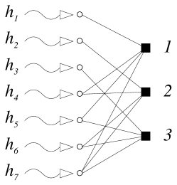
Figure 3: The information coming from the channel must be used for decoding the ${\cal H}_{2}(3)$ Hamming code: a pictorial view.

The decoding problem is to compute the probability for each transmitted bit $\sigma_{i}^{\rm in}$ to take the value $\sigma_{i}$, given the structure of the code and the received message $\underline{{\tt x}}^{\rm out}=[{\tt x}^{\rm out}_{1},\dots,{\tt x}^{\rm out}_{N}]^{\tt T}$. This is in general an intractable problem [3, 4]. Recently there has been a great interest in dealing with this problem using approximate message passing algorithms.

Message passing algorithms are iterative: at each step $t$ one keeps track of $M\overline{k}$ messages from the variable nodes to the check nodes $\{y^{(t)}_{\alpha\to i}\}$ and viceversa $\{x^{(t)}_{i\to\alpha}\}$. Messages can be thought to travel along the edges and computations to be executed at the nodes. A node computes the message to be sent along each one of the edges, using the messages received from the other (!) edges at the previous iteration (the variable nodes make also use of the log-likelihoods $h({\tt x}_{i}^{\rm out})$), cf. Fig. 4. At some point the iteration is stopped (there exists no general stopping criterion), and a choice for the bit $\sigma_{i}$ is taken using all the incoming messages (plus the log-likelihood $h({\tt x}_{i}^{\rm out})$).

The functions which define the “new” messages in terms of the “old” ones, can be chosen to optimize the decoder performances. A particularly interesting family is the following:

$$x^{(t+1)}_{i\to\alpha} = h_{i}+\sum_{\alpha^{\prime}\ni i:\,\alpha^{\prime}\neq\alpha}y^{(t)}_{\alpha^{\prime}\to i}\,$$ (2.8)

$$y^{(t+1)}_{\alpha\to i} = \frac{1}{\zeta}\,{\rm arctanh}\left[\prod_{j\in\alpha:\,j\neq i}\tanh\zeta x^{(t)}_{j\to\alpha}\right]\,,$$ (2.9)

where we used the notation $i\in\alpha$ whenever the bit $i$ belongs to the parity check $\alpha$. The messages $\{x^{(\cdot)}_{i\to\alpha}\}$ and $\{y^{(\cdot)}_{\alpha\to i}\}$ can be rescaled in such a way to eliminate the parameter $\zeta$ everywhere except in front of $h_{i}$. Therefore $\zeta$ allows to tune the importance given to the information contained in the received message.

After the convergence of the above iteration one computes the a posteriori log-likelihoods as follows:

$$H_{i}=h_{i}+\sum_{\alpha\ni i}y^{(\infty)}_{\alpha\to i}\,.$$ (2.10)

The meaning of the $\{H_{i}\}$ is analogous to the one of the $\{h_{i}\}$ (but for the fact that the $H_{i}$ incorporate the information coming from the structure of the code): the best guess for the bit $i$ is $\sigma_{i}=+1$ or $\sigma_{i}=-1$ depending whether $H_{i}>0$ or $H_{i}<0$.

The most popular choice for the free parameter $\zeta$ is $\zeta=1$: this algorithm has been invented separately by R. G. Gallager [15] in the coding theory context (and named the sum-product algorithm) and by D. Pearl [40] in the artificial intelligence context (and named the belief propagation algorithm). Also $\zeta=\infty$ is sometimes used (the max-product algorithm).

Figure 4: A graphic representation of the operations executed in a message passing algorithm. At the variable node $i$ (on the left): $x^{(t+1)}_{i\to 1}=F(y^{(t)}_{2\to i},y^{(t)}_{3\to i};h_{i})$. At the check node $\alpha$ (on the right): $y^{(t+1)}_{\alpha\to 1}=G(x^{(t)}_{2\to\alpha},x^{(t)}_{3\to\alpha},x^{(t)}_{4\to\alpha})$.

The alerted reader will notice that the Eqs. (2.8)-(2.9) are nothing but the cavity equations at inverse temperature $\zeta$ for a properly constructed spin model. This remark is the object of Refs. [41, 22].

In the analysis of the above algorithm it is convenient to assume that $\sigma^{\rm in}_{i}=+1$ for $i=1,\dots,N$. This assumption can be made without loss of generality if the channel is symmetric (i.e. if $Q({\tt x}|+1)=Q(-{\tt x}|-1)$). With this assumption the $h_{i}$ are i.i.d. random variables with density

$$p(h)\equiv Q({\tt x}(h)|+1)|{\tt x}^{\prime}(h)|\,,$$ (2.11)

where ${\tt x}(h)$ is the function which inverts Eq. (2.7). In the following we shall consider two particular examples of noisy channels, the generalization being straightforward:

• The binary erasure channel (BEC). In this case a bit can either be received correctly or erased. There are therefore three possible outputs: $\{+1,-1,0\}$. The transition probability is:

  $$Q({\tt x}^{\rm out}|+1)=\left\{\begin{array}[]{rl}(1-p)&\mbox{if }{\tt x}^{\rm out}=+1\,,\\ p&\mbox{if }{\tt x}^{\rm out}=0\,,\\ 0&\mbox{if }{\tt x}^{\rm out}=-1\,,\end{array}\right.\;\;\;Q({\tt x}^{\rm out}|-1)=\left\{\begin{array}[]{rl}0&\mbox{if }{\tt x}^{\rm out}=+1\,,\\ p&\mbox{if }{\tt x}^{\rm out}=0\,,\\ (1-p)&\mbox{if }{\tt x}^{\rm out}=-1\,.\end{array}\right.$$ (2.18)

  We get therefore the following distribution for the log-likelihoods: $p(h)=(1-p)\,\delta_{\infty}(h)+p\,\delta(h)$ (where $\delta_{\infty}$ is a Dirac delta function centered at $+\infty$). Let us recall that the capacity of the BEC is given by $C_{BEC}=1-p$: this means that a rate-$R$ code cannot assure error correction if $p>1-R$.

• The binary symmetric channel (BSC). The channel flips each bit independently with probability $p$. Namely

  $$Q({\tt x}^{\rm out}|+1)=\left\{\begin{array}[]{rl}(1-p)&\mbox{if }{\tt x}^{\rm out}=+1\,,\\ p&\mbox{if }{\tt x}^{\rm out}=-1\,,\end{array}\right.\;\;\;Q({\tt x}^{\rm out}|-1)=\left\{\begin{array}[]{rl}p&\mbox{if }{\tt x}^{\rm out}=+1\,,\\ (1-p)&\mbox{if }{\tt x}^{\rm out}=-1\,.\end{array}\right.$$ (2.24)

  The corresponding log-likelihood distribution is $p(h)=(1-p)\,\delta(h-h_{0})+p\,\delta(h+h_{0})$, with $h_{0}={\rm arctanh}(1-2p)$. The capacity of the BSC is $C_{BSC}=1-{\tt h}(p)$: a rate-$R$ code cannot correct errors if $p>\delta_{GV}(R)$.

It is quite easy [42, 34] to write a recursive equations for the probability distributions of the messages $\pi_{t}(x)$ and $\widehat{\pi}_{t}(y)$:

$$\pi_{t+1}(x) = \frac{1}{\overline{l}}\sum_{l=2}^{\infty}v_{l}l\int\!\prod_{i=1}^{l-1}dy_{i}\,\widehat{\pi}_{t}(y_{i})\,\int\!dh\,p(h)\;\delta\left(x-h-\sum_{i=1}^{l-1}y_{i}\right)\,,$$ (2.26)

$$\widehat{\pi}_{t+1}(y) = \frac{1}{\overline{k}}\sum_{k=3}^{\infty}c_{k}k\int\!\prod_{i=1}^{k-1}dx_{i}\,\pi_{t}(x_{i})\;\delta\left(y-\frac{1}{\zeta}\,{\rm arctanh}\left[\prod_{i=1}^{k-1}\tanh\zeta x_{i}\right]\right)\,.$$ (2.27)

These equations (usually called the density evolution equations) are correct for times $t\ll\log N$ due to the fact that the Tanner graph is locally tree-like. They allow therefore to predict whether, for a given ensemble of codes and noise level (recall that the noise level is hidden in $p(h)$) the algorithm is able to recover the transmitted codeword (for large $N$). If this is the case, the distributions $\pi_{t}(x)$ and $\widehat{\pi}_{t}(y)$ will concentrate on $x=y=+\infty$ as $t\to\infty$. In the opposite case the above iteration will converge to some distribution supported on finite values of $x$ and $y$.

BEC BSC $(k,l)$ $p_{c}$ $p_{d}$ $p_{c}$ $p_{d}(\zeta=1)$ $p_{d}(\zeta=2)$ $p_{d}(\zeta=\infty)$ $(6,3)$ $0.4882$ $0.4294$ $0.100$ $0.084$ $0.078$ $0.072$ $(10,5)$ $0.4995$ $0.3416$ $0.109$ $0.070$ $0.056$ $0.046$ $(14,7)$ $0.5000$ $0.2798$ $0.109$ $0.056$ $0.039$ $0.029$ $(6,5)$ $0.8333$ $0.5510$ $0.264$ $0.139$ $0.102$ $0.078$

Table 1: The statical and dynamical points for several regular codes and decoding algorithms, cf. Eqs. (2.8), (2.9).

In Tab. 1 we report the threshold noise levels for several regular codes, obtained using the density evolution method, together with the thresholds for the optimal decoding strategy, see Ref. [32].

Finally let us notice that the fixed point of the iteration (2.26)-(2.27) is the replica symmetric order parameter for the equivalent spin model.

3 Statistical mechanics formulation and the replica approach

We want to define a statistical mechanics model which describes the decoding problem. The probability distribution for the input codeword to be $\underline{\sigma}=(\sigma_{1},\dots,\sigma_{N})$ conditional to the received message, takes the form

$$P(\underline{\sigma})=\frac{1}{Z}\delta_{\mathbb{H}}[\underline{\sigma}]\,\exp\left\{\sum_{i=1}^{N}h_{i}\sigma_{i}\right\}\,,$$ (3.1)

where $\delta_{\mathbb{H}}[\underline{\sigma}]=1$ if $\underline{\sigma}$ satisfies the parity checks encoded by the matrix ${\mathbb{H}}$, cf. Eq. (2.1), and $\delta_{\mathbb{H}}[\underline{\sigma}]=0$ otherwise. Since we assume the input codeword to be $\underline{\sigma}^{\rm in}=(+1,+1,\dots,+1)$, the $h_{i}$ are i.i.d. with distribution $p(h)$.

We modify the probability distribution (3.1) in two ways:

1. We multiply the fields $h_{i}$ by a weight $\hat{\zeta}$. This allows us to tune the importance of the received message, analogously to Eqs. (2.8) and (2.9). This modification was already considered in Ref. [32]. Particularly important cases are $\hat{\zeta}=1$ and $\hat{\zeta}=0$.

2. We relax the constraints implied by the characteristic function $\delta_{\mathbb{H}}[\underline{\sigma}]$. More precisely, let us denote each parity check by the un-ordered set of bits positions $(i_{1},\dots,i_{k})$ which appears in it. For instance the three parity checks in the Hamming code ${\cal H}_{2}(3)$, cf. Eq. (2.5), are $(1,4,5,7)$, $(2,4,6,7)$, $(3,5,6,7)$. Moreover let $\Omega_{k}$ be the set of all parity checks involving $k$ bits (in the irregular ensemble the size of $\Omega_{k}$ is $Nc_{k}$). We can write explicitly the characteristic function $\delta_{\mathbb{H}}[\underline{\sigma}]$ as follows:

   $$\delta_{\mathbb{H}}[\underline{\sigma}]=\prod_{k=3}^{\infty}\prod_{(i_{1}\dots i_{k})\in\Omega_{k}}\delta(\sigma_{i_{1}}\cdots\sigma_{i_{k}},+1)\,,$$ (3.2)

   where $\delta(\cdot,\cdot)$ is the Kronecker delta function. Now it is very simple to relax the constraints by making the substitution $\delta(\sigma_{i_{1}}\cdots\sigma_{i_{k}},+1)\to\exp\{\beta[\sigma_{i_{1}}\cdots\sigma_{i_{k}}-1]\}$.

Summarizing the above considerations, we shall consider the statistical mechanics model defined by the Hamiltonian

$$H(\sigma)=-\sum_{k=3}^{\infty}\sum_{(i_{1}\dots i_{k})\in\Omega_{k}}\!\!\!\!(\sigma_{i_{1}}\cdots\sigma_{i_{k}}-1)\;\;\;-\;\frac{\hat{\zeta}}{\beta}\sum_{i=1}^{N}h_{i}\sigma_{i}\,,$$ (3.3)

at inverse temperature $\beta$.

We address this problem by the replica approach [43] The replicated partition function reads

$$\langle Z^{n}\rangle\sim\int\!\prod_{\vec{\sigma}}d\lambda(\vec{\sigma})d\widehat{\lambda}(\vec{\sigma})\,e^{-NS[\lambda,\widehat{\lambda}]}\,,$$ (3.4)

with the action

$$S[\lambda,\widehat{\lambda}] = \overline{l}\sum_{\vec{\sigma}}\lambda(\vec{\sigma})\widehat{\lambda}(\vec{\sigma})-\frac{\overline{l}}{\overline{k}}\sum_{k=3}^{\infty}c_{k}\sum_{\vec{\sigma}_{1}\dots\vec{\sigma}_{k}}J_{\beta}(\vec{\sigma}_{1},\dots,\vec{\sigma}_{k})\lambda(\vec{\sigma}_{1})\cdots\lambda(\vec{\sigma}_{k})-$$

$$-\sum_{l=2}^{\infty}v_{l}\log\left[\sum_{\vec{\sigma}}\widehat{\lambda}(\vec{\sigma})^{l}{\cal H}(\vec{\sigma})\right]-\overline{l}+\frac{\overline{l}}{\overline{k}}\,,$$

where

$$J_{\beta}(\vec{\sigma}_{1},\dots,\vec{\sigma}_{k})\equiv e^{\beta\sum_{a}(\sigma_{1}\dots\sigma_{k}-1)}\,,\;\;\;\;\;\;\;\;{\cal H}(\vec{\sigma})=\langle e^{\hat{\zeta}h\sum_{a}\sigma_{a}}\rangle_{h}\,,$$ (3.6)

$\langle\cdot\rangle_{h}$ being the average over $p(h)$. The order parameters $\lambda(\vec{\sigma})$ and $\widehat{\lambda}(\vec{\sigma})$ are closely related, at least in the replica symmetric approximation, to the distribution of messages in the decoding algorithm [32], cf. Eqs. (2.26), (2.27).

In the case of the BEC an irrelevant infinite constant must be subtracted from the action (3) in order to get finite results. This corresponds to taking

$${\cal H}_{BEC}(\vec{\sigma})\equiv p+(1-p)\delta_{\vec{\sigma},\vec{\sigma}_{0}}\,,$$ (3.7)

where $\vec{\sigma}_{0}=(+1,\dots,+1)$.

4 Binary erasure channel: analytical and numerical results

The binary erasure channel is simpler than the general case. Intuitively this happens because one cannot receive misleading indications concerning a bit. Nonetheless it is an important case both from the practical [44] and from the theoretical point of view [45, 34, 38].

4.1 The decoding algorithm

Iterative decoding algorithms for irregular codes were first introduced and analyzed within this context [38]. Belief propagation becomes particularly simple. Since the knowledge about a received bit is completely sure, the log-likelihoods $\{h_{i}\}$, cf. Eq. (2.7), take the values $h_{i}=+\infty$ (when the bit has been received) or $h_{i}=0$ (when it has been erased). Analogously the messages $\{x^{(t)}_{i\to\alpha}\}$ and $\{y^{(t)}_{\alpha\to i}\}$ must assume the same two values. The rules (2.8), (2.9) become

$$x^{(t+1)}_{i\to\alpha} = \left\{\begin{array}[]{rl}+\infty&\mbox{ if either }h_{i}=+\infty\mbox{ or }y^{(t)}_{\alpha^{\prime}\to i}=+\infty\mbox{ for some $\alpha^{\prime}\ni i$ (with $\alpha^{\prime}\neq\alpha$)},\\ 0&\mbox{otherwise,}\end{array}\right.$$ (4.3)

$$y^{(t+1)}_{\alpha\to i} = \left\{\begin{array}[]{rl}+\infty&\mbox{ if }x^{(t)}_{j\to\alpha}=+\infty\mbox{ for all the $j\in\alpha$ (with $j\neq i$)},\\ 0&\mbox{otherwise.}\end{array}\right.$$ (4.6)

There exists an alternative formulation [38] of the same algorithm. Consider the system of $M$ linear equations (2.1) and eliminate from each equation the received variables (which are known for sure to be $\tt 0$). You will obtain a new linear system. In some cases you may have eliminated all the variables of one equation, the equation is satisfied and can therefore be eliminated. For some of the other equations you may have eliminated all the variables but one. The remaining variable can be unambiguously fixed using this equation (since the received message is not misleading, this choice is surely correct). This allows to eliminate the variable from the entire linear system. This simple procedure is repeated until either all the variables have been fixed, or one gets stuck on a linear system such that all the remaining equations involve at least two variables (this is called a stopping set [45]).

Let us for instance consider the linear system defined by the parity check matrix (2.5). Suppose, in a first case, that the received message was $(\tt 0,\ast,\tt 0,\ast,\tt 0,\ast,\tt 0)$ (meaning that the bits of positions $2$, $4$, $6$ were erased). The decoding algorithm proceeds as follows:

$$\left\{\begin{array}[]{lcr}{\tt x}_{1}+{\tt x}_{4}+{\tt x}_{5}+{\tt x}_{7}&=&\tt 0\\ {\tt x}_{2}+{\tt x}_{4}+{\tt x}_{6}+{\tt x}_{7}&=&\tt 0\\ {\tt x}_{3}+{\tt x}_{5}+{\tt x}_{6}+{\tt x}_{7}&=&\tt 0\end{array}\right.\Rightarrow\left\{\begin{array}[]{lcr}{\tt x}_{4}&=&\tt 0\\ {\tt x}_{2}+{\tt x}_{4}+{\tt x}_{6}&=&\tt 0\\ {\tt x}_{6}&=&\tt 0\end{array}\right.\Rightarrow\left\{\begin{array}[]{lcr}\tt 0&=&\tt 0\\ {\tt x}_{2}&=&\tt 0\\ \tt 0&=&\tt 0\end{array}\right.\,.$$ (4.16)

In this case the algorithm succeeded in solving the decoding problem. Let us now see what happens if the received message is $(\ast,\tt 0,\ast,\tt 0,\ast,\tt 0,\ast)$:

$$\left\{\begin{array}[]{lcr}{\tt x}_{1}+{\tt x}_{4}+{\tt x}_{5}+{\tt x}_{7}&=&\tt 0\\ {\tt x}_{2}+{\tt x}_{4}+{\tt x}_{6}+{\tt x}_{7}&=&\tt 0\\ {\tt x}_{3}+{\tt x}_{5}+{\tt x}_{6}+{\tt x}_{7}&=&\tt 0\end{array}\right.\Rightarrow\left\{\begin{array}[]{lcr}{\tt x}_{1}+{\tt x}_{5}+{\tt x}_{7}&=&\tt 0\\ {\tt x}_{7}&=&\tt 0\\ {\tt x}_{3}+{\tt x}_{5}+{\tt x}_{7}&=&\tt 0\end{array}\right.\Rightarrow\left\{\begin{array}[]{lcr}{\tt x}_{1}+{\tt x}_{5}&=&\tt 0\\ \tt 0&=&\tt 0\\ {\tt x}_{3}+{\tt x}_{5}&=&\tt 0\end{array}\right.\,.$$ (4.26)

The algorithm found a stopping set. Notice that the resulting linear system may well have a unique solution (although this is not the case in our example), which can be found by means of simple polynomial algorithms [46]. Simply the iterative algorithm is unable to further reduce it.

The analysis of this algorithm [34] uses the density evolution equations (2.26), (2.27) and is greatly simplified because the messages $\{x^{(t)}_{i\to\alpha}\}$ and $\{y^{(t)}_{\alpha\to i}\}$ take only two values. Their distributions have the form:

$$\pi_{t}(x)=\rho_{t}\,\delta(x)+(1-\rho_{t})\,\delta_{\infty}(x)\;\;\;,\widehat{\pi}_{t}(x)=\hat{\rho}_{t}\,\delta(y)+(1-\hat{\rho}_{t})\,\delta_{\infty}(y)\,,$$ (4.27)

where $\delta_{\infty}(\cdot)$ is a delta function centered at $+\infty$. The parameters $\rho$ and $\hat{\rho}$ give the fraction of zero messages, respectively from variables to checks and from checks to variables. Using Eqs. (2.26) and (2.27), we get:

$$\rho_{t+1}=p\,\frac{v^{\prime}(\hat{\rho}_{t})}{v^{\prime}(1)}\;\,,\;\;\;\;\;\;\;\;\;\hat{\rho}_{t+1}=1-\frac{c^{\prime}(1-\rho_{t})}{c^{\prime}(1)}\,.$$ (4.28)

The initial condition $\rho_{0}=\hat{\rho}_{0}=1$ converges to the perfect recovery fixed point $\rho=\hat{\rho}=0$ if $p<p_{d}$. This corresponds to perfect decoding. For $p>p_{d}$ the algorithm gets stuck on a non-trivial linear system: $\rho_{t}\to\rho_{*}$, $\hat{\rho}_{t}\to\hat{\rho}_{*}$, with $0<\rho_{*},\hat{\rho}_{*}<1$. The two regimes are illustrated in Fig. 5.

Figure 5: The evolution of the iterative decoding algorithm on the BEC, cf. Eqs. (4.28). Here we consider the $(6,5)$ code: $\rho_{t+1}=p[1-(1-\rho_{t})^{5}]^{4}$. On the left $p=0.5<p_{d}$, on the right $p=0.6>p_{d}$.

4.2 Statical transition

In the spin model corresponding to the situation described above, we have two types of spins: the ones corresponding to correctly received bits, which are fixed by an infinite magnetic field $h_{i}=+\infty$; and the ones corresponding to erased bits, on which no magnetic field acts: $h_{i}=0$. We can therefore consider an effective model for the erased bits once the received ones are fixed to $+1$. This correspond somehow to what is done by the decoding algorithm: the received bits are set to their values in the very first step of the algorithm and remain unchanged thereafter.

Let us consider the zero temperature limit. If the system is in equilibrium, its probability distribution will concentrate on zero energy configurations: the codewords. We will have typically ${\cal N}_{\rm words}(p)\sim 2^{Ns_{\rm words}(p)}$ codewords compatible with the received message. Their entropy $s_{\rm words}(p)$ can be computed within the replica formalism, cf. App. A. The result is

$$s_{\rm words}(\rho,\hat{\rho};p)=\overline{l}\rho(1-\hat{\rho})+\frac{\overline{l}}{\overline{k}}\,c(1-\rho)+p\,v(\hat{\rho})-\frac{\overline{l}}{\overline{k}}\,,$$ (4.29)

which has to be maximized with respect to the order parameters $\rho$ and $\hat{\rho}$. The saddle point equations have exactly the same form as the fixed point equations corresponding to the dynamics (4.28), namely $\rho=pv^{\prime}(\hat{\rho})/v^{\prime}(1)$ and $\hat{\rho}=1-c^{\prime}(1-\rho)/c^{\prime}(1)$

The saddle point equations have two stable solutions, i.e. local maxima of the entropy (4.29): $(i)$ a completely ordered solution $\rho=\hat{\rho}=0$, with entropy $s_{\rm words}(0,0)=0$ (in some cases this solution becomes locally unstable above some noise $p_{loc}$); $(ii)$ (for sufficiently high noise level) a paramagnetic solution $\rho_{*},\hat{\rho}_{*}>0$. The paramagnetic solution appears at the same value $p_{d}$ of the noise above which the decoding algorithm gets stuck.

The fixed point to which the dynamics (4.28) converges coincides with the statistical mechanics result for $\rho_{*},\hat{\rho}_{*}$. However the entropy of the paramagnetic solution $s_{\rm words}(\rho_{*},\hat{\rho}_{*})$ is negative at $p_{d}$ and becomes positive only above a certain critical noise $p_{c}$. This means that the linear system produced by the algorithm continues to have a unique solution below $p_{c}$, although our linear time algorithm is unable find such a solution.

The “dynamical” critical noise $p_{d}$ is the solution of the following equation

$$p\frac{v^{\prime\prime}(\hat{\rho}_{*})c^{\prime\prime}(1-\rho_{*})}{v^{\prime}(1)c^{\prime}(1)}=-1\,,$$ (4.30)

where $\rho_{*}$ and $\hat{\rho}_{*}$ solve the saddle point equations. The statical noise can be obtained setting $s_{\rm words}(\rho_{*},\hat{\rho}_{*})=0$. Finally the completely ordered solution becomes locally unstable for

$$p_{loc}=\frac{c^{\prime}(1)v^{\prime}(1)}{v^{\prime\prime}(0)c^{\prime\prime}(1)}\,.$$ (4.31)

Figure 6: The phase diagram of the family of codes with generating polynomials $c(x)=\alpha x^{4}+(1-\alpha)x^{6}$, $v(x)=\alpha x^{2}+(1-\alpha)x^{3}$. The dashed line gives the local stability threshold for the completely ordered ferromagnetic phase. The continuous and dot-dashed lines refer (respectively) to the static and dynamic critical points $p_{c}(\alpha)$ and $p_{d}(\alpha)$.

As an example let us consider the one-parameter family of $R=1/2$ codes specified by the following generating polynomials: $c(x)=\alpha x^{4}+(1-\alpha)x^{6}$, $v(x)=\alpha x^{2}+(1-\alpha)x^{3}$. This is an irregular code which smoothly interpolates between the regular $(6,3)$ and $(4,2)$ codes. The local stability threshold is given by

$$p_{loc}(\alpha)=\frac{(3-\alpha)^{2}}{6\alpha(5-3\alpha)}\,.$$ (4.32)

The dynamical and critical curves $p_{d}(\alpha)$ and $p_{c}(\alpha)$ are reported in Fig. 6. Notice that the $\alpha$ value where $p_{d}(\alpha)$ reaches its maximum, corresponding to the best code in this family, is neither 0 nor 1. This is a simple example showing that irregular codes ($0<\alpha<1$) are generally superior to regular ones ($\alpha=0$ or $\alpha=1$ in this example). Notice also that above the tricritical point $\alpha_{t}\approx 0.79301412$, $p_{t}\approx 0.39057724$ the three curves $p_{loc}(\alpha)$, $p_{c}(\alpha)$ and $p_{d}(\alpha)$ coincide. In the following we shall study in some detail the $\alpha=0$ case, which corresponds to a regular $(6,3)$ code, the corresponding critical and dynamical points $p_{c}$ and $p_{d}$ are given in Tab. 1.

4.3 Dynamical transition

The dynamical transition is not properly described within the replica symmetric treatment given above. Indeed, the paramagnetic solution cannot be considered, between $p_{d}$ and $p_{c}$, as a metastable state because it has negative entropy. One cannot therefore give a sensible interpretation of the coincidence between the critical noise for the decoding algorithm, and the appearance of the paramagnetic solution.

Before embarking in the one step replica symmetry-breaking (1RSB) calculation, let us review some well-known facts [47, 48]. Let us call $m\phi(\beta,m)$ the free energy of $m$ weakly coupled “real” replicas times beta. This quantity can be computed in 1RSB calculation. In the limit $\beta\to\infty$, with $m\beta=\mu$ fixed, we have $m\phi(\beta,m)\to\mu\phi(\mu)$. The number of metastable states with a given energy density $\epsilon$ is

$${\cal N}_{MS}(\epsilon)\sim e^{N\Sigma(\epsilon)}\,,$$ (4.33)

where the complexity $\Sigma(\epsilon)$ is the Legendre transform of the $m$ replicas free energy:

$$\Sigma(\epsilon)=\left.\mu\epsilon-\mu\phi(\mu)\right|_{\epsilon=\partial[\mu\phi(\mu)]}\,.$$ (4.34)

The (zero temperature) dynamic energy $\epsilon_{d}$ and the static energy $\epsilon_{s}$ are, respectively, the maximum and the minimum energy such that $\Sigma(\epsilon)\geq 0$.

The static energy is obtained by solving the following equations:

$$\left\{\begin{array}[]{c}\epsilon_{s}=\phi(\mu)\,,\\ \partial\phi(\mu)=0\,,\end{array}\right.$$ (4.37)

which corresponds to the usual prescription of maximizing the free energy over the replica symmetry breaking parameter $m$ [43]. The dynamic energy is given by

$$\left\{\begin{array}[]{c}\epsilon_{d}=\partial[\mu\phi(\mu)]\,,\\ \partial^{2}[\mu\phi(\mu)]=0\,.\end{array}\right.$$ (4.40)

Finally, if $\epsilon_{s}=0$ the complexity of the ground state is $\Sigma(0)=-\lim_{\mu\to\infty}\mu\phi(\mu)$.

We weren’t able to exactly compute the 1RSB free energy $\phi(\mu)$. However excellent results can be obtained within an “almost factorized” variational Ansatz, cf. App. A.2. The picture which emerges is the following:

• In the low noise region ($p<p_{d}$), no metastable states exist. Local search algorithms should therefore be able to recover the erased bits.

• In the intermediate noise region ($p_{d}<p<p_{c}$) an exponentially large number of metastable states appears. They have energy densities $\epsilon$ in the range $\epsilon_{s}<\epsilon<\epsilon_{d}$, with $\epsilon_{s}>0$. Therefore the transmitted codeword is still the only one compatible with the received message. Nonetheless a large number of extremely stable pseudo-codewords stop local algorithms. The number of violated parity checks in these codewords cannot be reduced by means of local moves.

• Above $p_{c}$ we have $\epsilon_{s}=0$: a fraction of the metastable states is made of codewords. Moreover $\Sigma(0)$ (which gives the number of such codewords) coincides with the paramagnetic entropy $s_{\rm words}(\rho_{*},\hat{\rho}_{*})$ computed in the previous Section.

Figure 7: The complexity $\Sigma(\epsilon)$ for (from top to bottom) $p=0.45$ (below $p_{c}$), $p=0.5$, and $p=0.55$ (above $p_{c}$).

As an illustration, let us consider the $(6,3)$ regular code. In Fig. 7 we plot the resulting complexity curves $\Sigma(\epsilon)$ for three different values of the erasure probability $p$.

Figure 8: Left-hand frame: the static and dynamic energies $\epsilon_{s}$ and $\epsilon_{d}$ of the metastable states (respectively, solid and dashed lines). Right-hand frame: the total complexity $\max_{\epsilon}\Sigma(\epsilon)$ and the zero energy complexity $\Sigma(0)$.

In Fig. 8, left frame, we report the static and dynamic energies $\epsilon_{s}$ and $\epsilon_{d}$ as functions of $p$. In the right frame we present the total complexity $\Sigma_{{\rm tot}}\equiv\max_{\epsilon}\Sigma(\epsilon)=\Sigma(\epsilon_{d})$, and the zero energy complexity $\Sigma(0)$.

4.4 Numerical results

In order to check analytical predictions and to better illustrate the role of metastable states, we have run a set of Monte Carlo simulations, with Metropolis dynamics, on the Hamiltonian (3.3) of the (6,3) regular code for the BEC. Notice that local search algorithms for the decoding problem have been already considered by the coding theory community [49].

We studied quite large codes ($N=10^{4}$ bits), and tried to decode it (i.e. to find a ground state of the corresponding spin model) with the help of simulated annealing techniques [50]. For each value of $p$, we start the simulation fixing a fraction $(1-p)$ of spins to $\sigma_{i}=+1$ (this part will be kept fixed all along the run). The remaining $pN$ spins are the dynamical variables we change during the annealing in order to try to satisfy all the parity checks. The energy of the system counts the number of unsatisfied parity checks.

The cooling schedule has been chosen in the following way: $\tau$ Monte Carlo sweeps (MCS)  at each of the 1000 equidistant temperatures between $T=1$ and $T=0$. The highest temperature is such that the system very rapidly equilibrates on the paramagnetic energy $\epsilon_{P}(T)$. Typical values for $\tau$ are from 1 to $10^{3}$.

Notice that, for any fixed cooling schedule, the computational complexity of the simulated annealing method is linear in $N$. Then we expect it to be affected by metastable states of energy $\epsilon_{d}$, which are present for $p>p_{d}$: the energy relaxation should be strongly reduced around $\epsilon_{d}$ and eventually be completely blocked.

Figure 9: Energy relaxation for the Hamiltonian of the (6,3) regular code during the simulated annealing with $\tau$ MCS per temperature and 1000 equidistant temperatures in $[0,1]$

In order to illustrate how the system relaxes during the simulated annealing we show in Fig. 9 the energy density as a function of the temperature for $p=0.4$ (left) and $p=0.6$ (right) and various cooling rates, $\tau=10,10^{2},10^{3}$ (each data set is the average over many different samples).

For $p=0.4<p_{d}$ the final energy strongly depends on the cooling rate and the slowest cooling procedure is always able to bring the system on the ground state, corresponding to the transmitted codeword. Decoding by simulated annealing is therefore successful.

For $p=0.6>p_{d}$ the situation drastically changes. Below a temperature $T_{d}$ (marked by an arrow in Fig. 9, right frame) there is an almost complete stop of the energy relaxation. $T_{d}$ marks the dynamical transition and the corresponding energy $\epsilon_{d}(T_{d})=\epsilon_{P}(T_{d})$ is called the threshold energy. The energy of threshold states still varies a little bit with temperature, $\epsilon_{d}(T)$, and the final value reached by the simulated annealing algorithm is its zero-temperature limit $\epsilon_{d}(0)=\epsilon_{d}$. Remember that, by construction, ground states of zero energy are present for any $p$ value, but they become unreachable for $p>p_{d}$, because they become shielded by metastable states of higher energy.

Figure 10: Lowest energies reached by the simulated annealing. Errors are sample to sample fluctuations.

We show in Fig. 10 the lowest energy reached by the simulated annealing procedure for different $p$ and $\tau$ values. While for $p<p_{d}$ all parity checks can be satisfied and the energy relaxes to zero in the limit of a very slow cooling, for $p\geq p_{d}$ the simulation get stuck in a metastable state of finite energy, that is with a number of unsatisfied parity checks of order $N$. The agreement with the analytic prediction (dotted line) is quite good everywhere, but very close to $p_{d}$.

Discrepancies between analytical predictions and numerical results may be very well due to finite-size effects in the latter. One possible explanation for large finite-size effects near the dynamic critical point $p_{d}$ is the following. Metastable states of energy $\epsilon_{d}$ are stable under any local dynamic, which may flip simultaneously only a finite number of spins, and under global dynamics flipping no more than $\omega N$ spins simultaneously. Physical intuition (threshold states become more robust increasing $p$) imply that the function $\omega(p)$ must monotonously increase for $p\in[p_{d},1]$. Moreover, continuity reasons tell us that $\omega(p_{d})=0$. The fact that $\omega(p)$ is very small close to $p_{d}$, together with the fact that in numerical simulations we are restricted to finite values of $N$, allow the local Monte Carlo dynamic to relax below the analytical predicted threshold energy. A more detailed characterization of this effect is presently under study and will be presented in a forthcoming publication.

5 The general channel: analytical and numerical results

We considered the case of a general noisy channel using two different approaches: a finite-temperature and a zero-temperature approach. While the first one offers a clear connection with the dynamics of decoding-by-annealing algorithm, the second one gives a nice geometrical picture of the situation.

5.1 Finite temperature

Suppose you received some message encoded using a Gallager code and you want to decode it, but no one explained to you the belief propagation algorithm, cf. Eqs. (2.8), (2.9).

A physicist idea would be the following. Write the corresponding Hamiltonian $H(\underline{\sigma})$, see Eq. (3.3), and run a Monte Carlo algorithm at inverse temperature $\beta$. If you wait enough time, you will be able to sample the configuration $\underline{\sigma}$ according to the Boltzmann distribution $P_{\beta}(\underline{\sigma})\propto e^{-\beta H(\underline{\sigma})}$. Then cool down the system adiabatically: i.e. change the temperature according to some schedule $\{\beta_{1},\beta_{2},\dots,\}$ with $\beta_{k}\uparrow\infty$, waiting enough time at each temperature for the system to equilibrate.

As $\beta\to\infty$ the Boltzmann measure of the Hamiltonian (3.2) concentrates on the codewords (for which the exchange term in Eq. (3.2) is equal to zero). Moreover each codeword is given a weight which depends on its likelihood. In formulae:

$$\lim_{\beta\to\infty}P_{\beta}(\underline{\sigma})=\frac{1}{Z_{\hat{\zeta}}}\,P(\underline{\sigma}|\underline{{\tt x}}^{\rm out})^{\hat{\zeta}}\,,$$ (5.1)

where $P(\underline{\sigma}|\underline{{\tt x}}^{\rm out})$ is the probability for $\underline{\sigma}$ to be the transmitted codeword, conditional to the received message $\underline{{\tt x}}^{\rm out}$, and $Z_{\hat{\zeta}}$ is a normalization constant. Therefore when $\beta\gg 1$, our algorithm will sample a codeword with probability proportional to $P(\underline{\sigma}|\underline{{\tt x}}^{\rm out})^{\hat{\zeta}}$. For good codes below the critical noise threshold $p_{c}$, the likelihood $P(\underline{\sigma}|\underline{{\tt x}}^{\rm out})$ is strongly concentrated on the correct input codeword. Therefore the system will spend most of its time on the correct codeword as soon as $\beta\gg 1$ and $\hat{\zeta}\geq 1$ (for $\hat{\zeta}<1$, $p_{c}$ has a non-trivial dependence on $\hat{\zeta}$, cf. Ref. [32]).

This algorithm will succeed as long as we are able to keep the system in equilibrium at all temperatures down to zero. If some form of ergodicity breaking is present this may take an exponentially (in the size $N$) long time. Let us suppose to spend an $O(N)$ computational time at each temperature $\beta_{i}$ of the annealing schedule (this is what happens in Nature). We expect to be able to equilibrate the system only at low enough noise (let us say for $p<p_{d}(\hat{\zeta})$), when the magnetic field in Eq. (3.3) is strong enough for single out a unique ergodic component.

5.1.1 The random linear code limit

Some intuition on the static phase diagram can be gained by looking at the $k,l\to\infty$ limit with rate $R=1-l/k$ fixed, cf. App. B.1.1. Unhappily, in this limit the dynamic phase transition disappears: the decoding algorithm is always unsuccessful, as can be understood by looking at Eqs. (2.8)-(2.9). This phenomenon is analogous to what happens in the random energy model (REM) [51]: the dynamic transition is usually said to occur at infinite temperature. We refer to Sec. 5.2.1 for further clarifications of this point.

There exist a paramagnetic and a ferromagnetic phases, with free energy densities

$$f_{P} = -\frac{1}{\beta}\langle\log(2\cosh\hat{\zeta}h)\rangle_{h}+\frac{1-R}{\beta}\log(1+\tanh\beta)\,,$$ (5.2)

$$f_{F} = -\frac{\hat{\zeta}}{\beta}\langle h\rangle_{h}\,.$$ (5.3)

One must be careful in computing the entropy because of the explicit dependence of the Hamiltonian (3.2) upon the temperature. The result is that the ferromagnetic phase has zero entropy $s_{F}=0$, while the entropy of the paramagnetic phase is

$$s_{P} = \langle\log(2\cosh\hat{\zeta}h)\rangle_{h}-\langle\hat{\zeta}h\tanh\hat{\zeta}h\rangle_{h}-$$

$$-(1-R)\log(1+\tanh\beta)+(1-R)\beta(1-\tanh\beta)\,.$$

Figure 11: The phase diagram for the model (3.2) in the limit $k,l\to\infty$ with $R=1-l/k$ fixed. Here we consider $R=1/6$ and $\hat{\zeta}=1$ (on the left) and $1.5$ (on the right). The rightmost (i.e. noisier) point for which the ferromagnetic phase is globally stable is always at $\beta=\infty$, $p=\delta_{GV}(R)\approx 0.264$. Along the dashed line the entropy of the paramagnetic phase vanishes.

In the low-temperature, low-noise region the paramagnetic entropy $s_{P}$ becomes negative. This signals a REM-like glassy transition [51]. The spin glass free energy is obtained by maximizing over the RSB parameter $m$ (with $0\leq m\leq 1$) the following expression

$$f_{SG}(m)=-\frac{(1-R)}{\beta m}\log(1+e^{-2\beta m})-\frac{1}{m}\langle\log(2\cosh m\hat{\zeta}h)\rangle_{h}\,.$$ (5.5)

The generic phase diagram is reported in Fig. 11. At high temperature, as the noise level is lowered the system undergoes a paramagnetic-ferromagnetic transition and concentrates on the correct codeword. At low temperature an intermediate glassy phase may be present (for $\hat{\zeta}>1$): the system concentrates on a few incorrect configurations.

5.1.2 Theoretical dynamical line

The existence of metastable states can be detected within the replica formalism by the so-called marginal stability condition. One considers the saddle point equations for the 1RSB order parameter, fixing the RSB parameter $m=1$, cf. App. B. The dynamical temperature $T_{d}(p)$ is the highest temperature for which a “non-trivial” solution of the equation exists. At this temperature ergodicity of the physical dynamics breaks down (at least this is what happens in infinite connectivity mean field models) and we are no longer able to equilibrate the system within an $O(1)$ physical time (i.e. an $O(N)$ computational time).

We looked for a solution of Eqs. (B.3)-(B.6) using the population dynamics algorithm of Ref. [19]. We checked the “non-triviality” of the solution found by considering the variance of the distributions $\rho(x)$, $\hat{\rho}(y)$ (more precisely of the populations which represent such distributions in the algorithm).

Figure 12: The dynamical phase transition for a regular $(6,5)$ code (cf. Eq. (3.2) with $k=6$ and $l=5$) with $\hat{\zeta}=1$.

We consider the $(6,5)$ regular code because it has well separated statical and dynamical thresholds $p_{c}$ and $p_{d}$, cf. Tab. 1. The resulting dynamical line for the Hamiltonian (3.2) with $\hat{\zeta}=1$, is reported in Fig. 12. The dynamic temperature $T_{d}(p)$ drops discontinuously below a noise $p_{d}(\hat{\zeta})$: for $p<p_{d}(\hat{\zeta})$ the dynamical transition disappears and the system can be equilibrated in linear computational time down to zero temperature. We get $p_{d}(1)\approx 0.14$, which is in good agreement with the coding theory results, cf. Tab. 1

5.1.3 Numerical experiments

We have repeated for the BSC the same kind of simulations already presented at the end of Sec. 4.4 for the BEC.

We have run a set of simulated annealings for the Hamiltonian 3.3 of the (6,5) regular code. System size is $N=12000$ and the cooling rates are the same as for the BEC, the only difference being the starting and the ending temperatures, which are now $T=1.2$ and $T=0.2$ (plus a quench from $T=0.2$ to $T=0$ at the end of each cooling). This should not have any relevant effect because $0.2\ll T_{d}\approx 0.6$.

The important difference with respect to the BEC case is that now we have no fixed spins, all $N$ spins are dynamical variables subject to a random external field of intensity $h=(1/\beta){\rm arctanh}(1-2p)$, cf. Eq. (3.3).

Also here, as in the case of the BEC, the energy relaxation for $p>p_{d}$ undergoes a drastic arrest when the temperature is reduced below the dynamical transition at $T_{d}$, see Fig. 13.

Figure 13: Energy relaxation for the Hamiltonian of the (6,5) regular code during the simulated annealing with $\tau$ MCS per temperature and 1000 equidistant temperatures in $[0.2,1.2]$. Notice that, in both cases $p>p_{d}$. The dot-dashed line is the theoretical prediction for the paramagnetic exchange energy.

Unfortunately, in this case, we are not able to calculate analytically the threshold energy $\epsilon_{d}(0)$, but only the dynamical critical temperature $T_{d}$ and then the threshold energy at the transition $\epsilon_{d}(T_{d})$ which is higher than $\epsilon_{d}(0)$. The difference $\Delta\epsilon=\epsilon_{d}(T_{d})-\epsilon_{d}(0)$ is usually not very large (see e.g. the BEC case), but it becomes apparent when $p$ is decreased towards $p_{d}$. Indeed for $p=0.25$ (Fig. 13 left) the Metropolis dynamics is still able to relax the system for temperatures below $T_{d}$ and then it reaches an energy well below $\epsilon_{d}(T_{d})$. On the other hand for $p=0.5$ (Fig. 13 right), where $\Delta\epsilon$ is small the relaxation below $T_{d}$ is almost absent and the analytic prediction is much more accurate. Notice that for this case we have run a still longer annealing with $\tau=10^{4}$: the asymptotic energy is very close to that for $\tau=10^{3}$ and hardly distinguishable from the analytical prediction.

Figure 14: Lowest energies reached by the simulated annealings. Errors are sample to sample fluctuations. The theoretical prediction $\epsilon_{d}(T_{d})$ is computed using the results in Fig. 12 for $T_{d}(p)$.

In Fig. 14 we report the lowest energy reached by the simulated annealing for many values of $p$ and $\tau=10,10^{2},10^{3}$, together with the analytic calculation for the threshold energy at $T_{d}$. This analytical value is an upper bound for the true threshold energy $\epsilon_{d}(0)$ where linear algorithms should get stuck, but it gives very accurate predictions for large $p$ values where $\Delta\epsilon$ is very small. In the region of small $p$ a more complete calculation is needed.

5.2 Zero temperature

This approach follows from a physical intuition that is slightly different from the one explained in the previous paragraphs. Once again we will formulate it algorithmically. For sake of simplicity we shall refer, in this Section, to the BSC. We refer to the Appendix (B.2) for more general formulae.

The overlap between the transmitted codeword and the received message

$$q^{\rm in,out}=\frac{1}{N}\sum_{i=1}^{N}\sigma^{\rm in}_{i}\sigma^{\rm out}_{i}\,,$$ (5.6)

is, typically, $q^{\rm in,out}=1-2p$. Given the received message, one can work in the subspace of all the possible configurations which have the prescribed overlap with it, i.e. all the $\underline{\sigma}$ such that $(1/N)\sum_{i=1}^{N}\sigma_{i}\sigma_{i}^{\rm out}\approx(1-2p)$. Once this constraint has been imposed (for instance in a Kawasaki-like Monte Carlo algorithm) one can restrict himself to the exchange part of the Hamiltonian (3.2) $H_{\rm exch}(\underline{\sigma})=-\sum_{k}\sum_{(i_{1}\dots i_{k})}\sigma_{i_{1}}\cdots\sigma_{i_{k}}$ and apply the cooling strategy already described in the previous Section.

Below the static transition $p_{c}$ there exists a unique codeword having overlap $(1-2p)$ with the received signal. This is exactly the transmitted one $\underline{\sigma}^{\rm in}$. This means that $\underline{\sigma}^{\rm in}$ is the unique ground state of $H_{\rm exch}(\underline{\sigma})$ in the subspace we are considering. If we are able to keep our system in equilibrium down to $T=0$, the cooling procedure will finally yield the correct answer to the decoding problem. Of course, if metastable states are encountered in this process, the time required for keeping the system in equilibrium diverges exponentially in the size.

We expect the number of such states to be exponentially large:

$${\cal N}_{MS}(\epsilon,q|p)\sim e^{N\Sigma_{p}(\epsilon,q)}\,,$$ (5.7)

where $\epsilon$ is the exchange energy density $H_{\rm exch}(\underline{\sigma})/N$. Notice that we emphasized the dependence of these quantities upon the noise level $p$. In fact the noise level determines the statistics of the received message $\underline{\sigma}^{\rm out}$. The static threshold is the noise level at which an exponential number of codewords with the same overlap as the correct one ($q=1-2p$) appears: $\Sigma_{p}(0,1-2p)>0$. The dynamic transition occurs where metastable states with the same overlap begin to exist: $\Sigma_{p}(\epsilon,1-2p)>0$ for some $\epsilon>0$.

5.2.1 The random linear code limit

It is quite easy to compute the complexity $\Sigma_{p}(\epsilon,q)$ in the limit $k,l\to\infty$ with rate $R=1-l/k$ fixed. In particular, the zeroth order term in a large $k,l$ expansion can be derived by elementary methods.

In this limit we expect the regular $(k,l)$ ensemble to become identical to the random linear code (RLC) ensemble. The RLC ensemble is defined by taking each element of the parity check matrix ${\mathbb{H}}$, cf. Eq. (2.1) to be $0$ or $1$ with equal probability. Distinct elements are considered to be statistically independent.

Let us compute the number of configurations $\underline{\sigma}$ having a given energy and overlap with the received message $\underline{\sigma}^{\rm out}$. Given a bit sequence $\underline{{\tt x}}\neq\underline{\tt 0}$, the probability that $L$ out of $M$ equations ${\mathbb{H}}\underline{{\tt x}}=\underline{\tt 0}$ are violated is

$$P_{L,\underline{{\tt x}}}=\left(\begin{array}[]{c}M\\ L\end{array}\right)2^{-M}\,.$$ (5.10)

Therefore the expected number of configurations $\underline{{\tt x}}$ which violate $L$ checks and have Hamming distance $W$ from the received message $\underline{{\tt x}}^{\rm out}$ is

$$\overline{{\cal N}_{W,L}}=\delta_{W,W_{\underline{{\tt x}}^{\rm out}}}\delta_{L,0}[1-2^{-M}]+\left(\begin{array}[]{c}N\\ W\end{array}\right)\left(\begin{array}[]{c}M\\ L\end{array}\right)2^{-M}\,,$$ (5.15)

where $W_{\underline{{\tt x}}^{\rm out}}$ is the weight of $\underline{{\tt x}}^{\rm out}$, i.e. its Hamming distance from $\underline{\tt 0}$. Notice that, up to exponentially small corrections, the above expression does not depend on $\underline{{\tt x}}^{\rm out}$.

Introducing the overlap $q=1-2W/N$ and the exchange energy density $\epsilon=2L/N$, we get $\overline{{\cal N}_{W,L}}\sim 2^{N\tilde{\Sigma}(\epsilon,q)}$ with

$$\tilde{\Sigma}(\epsilon,q)={\tt h}[(1-q)/2]+(1-R)\,{\tt h}[\epsilon/2(1-R)]-(1-R)\,.$$ (5.16)

The typical number ${\cal N}^{\rm typ}_{W,L}$ of such configurations can be obtained through the usual REM construction: ${\cal N}^{\rm typ}_{W,L}\sim 2^{N\tilde{\Sigma}(\epsilon,q)}$ when $\tilde{\Sigma}(\epsilon,q)\geq 0$ and ${\cal N}^{\rm typ}_{W,L}=0$ otherwise.

Now we are interested in picking, among all the configurations having a given energy density $\epsilon$ and overlap $q$, the metastable states. In analogy with the REM, this can be done by eliminating all the configurations such that $\partial_{\epsilon}\tilde{\Sigma}(\epsilon,q)<0$. In other words, the number of metastable states is ${\cal N}_{MS}(\epsilon,q)\sim 2^{N\Sigma(\epsilon,q)}$ with $\Sigma(\epsilon,q)=\tilde{\Sigma}(\epsilon,q)$ when $\tilde{\Sigma}(\epsilon,q),\partial_{\epsilon}\tilde{\Sigma}(\epsilon,q)>0$, $\Sigma(\epsilon,q)=-\infty$ otherwise.

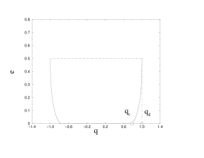
Figure 15: Metastable states in the random linear code limit for $R=1/2$: their number is exponential between the continuous and the dashed lines. It vanishes discontinuously when the dashed line is crossed and continuously when the continuous line is crossed. The critical and dynamical overlaps are related to the statical and critical noise by $q_{c,d}=1-2p_{c,d}$. In this limit $p_{d}=0$ and $p_{c}=\delta_{GV}(1/2)\approx 0.110025$.

In Fig. 15 we plot the region of the $(\epsilon,q)$ plane for which $\Sigma(\epsilon,q)>0$, for $R=1/2$ codes. Notice that, in this limit $\Sigma(\epsilon,q)$ does not depend on the received message $\underline{\sigma}^{\rm out}$ (and, therefore, is independent of $p$). As expected we get $p_{c}=\delta_{GV}(R)$ and $p_{d}=0$.

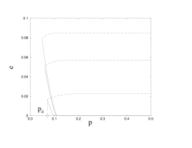
Figure 16: Metastable states for regular $(k,l)$ codes in a large-$k$,$l$ expansion, at fixed rate $R=1/2$. We consider (from bottom to top) $(k,l)=(6,3)$, $(10,5)$, $(14,7)$. On the left we show the region where $\Sigma_{p=0}(\epsilon,q)>0$. On the right we consider instead $\Sigma_{p}(\epsilon,1-2p)$.

In order to get the first non-trivial estimate for the dynamical point $p_{d}$, we must consider the next term in the above expansion. This correction can be obtained within the replica formalism, see App. B.2.1. In Fig. 16 we reproduce contour of the region $\{(\epsilon,q):\Sigma_{p}(\epsilon,q)>0\}$ for a few regular codes of rate $R=1/2$: $(k,l)=(6,3)$,$(10,5)$,$(14,7)$. The main difference between these curves and the exact results, cf. Sec. 5.2.2, is the convexity of the upper boundary of the $\Sigma_{p}(\epsilon,q)>0$ region (dashed lines in Figs. 15 and 16).

The corresponding estimates for $p_{c}$ and $p_{d}$ are reported in Tab. 2.

$(k,l)$ $p_{c}$ $p_{d}(1)$ $(6,3)$ $0.097$ $0.071$ $(10,5)$ $0.108$ $0.060$ $(14,7)$ $0.109$ $0.049$ $(6,5)$ $0.264$ $0.108$

Table 2: Dynamical and statical thresholds at the first nontrivial order in a large $k$,$l$ expansion, cf. Tab. 1.

5.2.2 The complete calculation

The full 1RSB solution for can be obtained through the population dynamics method [19]. Here, as in Sec. 5.1.2, we focus on the example of the $(6,5)$ code. In Fig. 17 we plot the configurational entropy as a function of the energy of the states along the lines of constant $q$, together with the corresponding results obtained within a simple variational approach, cf. App. B.2.2. The approximate treatment is in quantitative agreement with the complete calculation for $\epsilon<\epsilon_{d}$, but predicts a value for the threshold energy which is larger than the correct one: $\epsilon_{d}^{var}>\epsilon_{d}$. Here $\epsilon_{d}^{var}\approx 0.127$ and almost $p$-independent.

Unhappily the estimate of the dynamic energy obtained from this curves is not very precise. Moreover, at least two more considerations prevent us from comparing these results with the ones of simulated annealing simulations, cf. Sec. 5.1.3: $(i)$ In our annealing experiments the overlap with the received message $\underline{\sigma}^{\rm out}$ is free to fluctuate; $(ii)$ We cannot exclude the 1RSB solution to become unstable at low temperature.

However the population dynamics solution give the estimate $p_{d}\lesssim 0.155$. This allows us to confirm that the point $p_{d}=0.139$ where the decoding algorithm fails to decode, cf. Tab. 1, coincides with the point where the metastable states appear.

Figure 17: The configurational entropy versus the energy for the $(6,5)$ regular code. Symbols refer to various noise levels. From top to bottom $p=0.5,0.4,0.35,0.3,0.25,0.2,0.18,0.155$. Continuous lines give the result of a variational computation, cf. App. B.2.2.

6 Conclusion

We studied the dynamical phase transition for a large class of diluted spin models in a random field, the main motivation being their correspondence with very powerful error correcting codes.

In a particular case, we were able to show that the dynamic critical point coincides exactly with the critical noise level for an important class of decoding algorithms, cf. Sec. 4 and App. A. For a general model of the noisy channel, we couldn’t present a completely explicit proof of the same statement. However, within numerical precision, we obtain identical values for the algorithmic and the statistical mechanics thresholds.

It may be worth listing a few interesting problems which emerge from our work:

• Show explicitly that the identity between statistical mechanics and algorithmic thresholds holds in general. From a technical point of view, this is a surprising fact because the two thresholds are obtained, respectively, within a replica symmetric, cf Eqs. (2.26), (2.27), and a one-step replica symmetry breaking calculations.

• We considered message-passing and simulated annealing algorithms. Extend the above analysis to other classes of algorithm (and, eventually, to any linear time algorithm).

• Message passing decoding algorithms get stuck because they are unable to decode some fraction of the received message, the “hard” bits, while they have been able to decode the other ones, the “easy” bits, cf. App. A.2.1. A closer look at this heterogeneous behavior would be very fruitful.

It is a pleasure to thank R. Zecchina who participated to the early stages of this work.

Appendix A Calculations: binary erasure channel

In this Appendix we give the details of the replica calculation for the BEC. Notice that although we use the regular $(6,3)$ code as a generic example, all the computations are presented for general degree distributions $\{c_{k}\}$ and $\{v_{l}\}$.

A.1 Replica symmetric approximation

The replica symmetric calculation is correct [32] as long as we focus on codewords (i.e. on zero energy configurations). The main reason is the Nishimori symmetry [53, 54, 55] which holds at $\beta=\infty$ and $\hat{\zeta}=1$ for the model (3.3). Therefore the replica symmetric approximation gives access the correct noise level $p_{c}$ for the statical phase transition. Although such computations have been already considered in Refs. [25, 32], it is interesting to review them for the BEC, which allows for a cleaner physical interpretation. Moreover here we generalize the already published results by considering a generic irregular construction.

We parametrize the order parameters $\lambda(\vec{\sigma})$, $\widehat{\lambda}(\vec{\sigma})$, cf. Eq. (3) using the Ansatz

$$\lambda(\vec{\sigma})=\int\!d\pi(x)\frac{e^{\beta x\sum_{a}\sigma^{a}}}{(2\cosh\beta x)^{n}}\,,\;\;\;\;\;\;\;\;\widehat{\lambda}(\vec{\sigma})=\int\!d\widehat{\pi}(y)\frac{e^{\beta y\sum_{a}\sigma^{a}}}{(2\cosh\beta y)^{n}}\,,$$ (A.1)

where we adopted the notation $\int\!d\pi(x)\,(\cdots)\equiv\int\!dx\,\pi(x)\,(\cdots)$. It is easy to see that the order parameters have the form

$$\pi(x)=(1-p)\delta_{\infty}(x)+p\,\rho(x)\,,\;\;\;\;\;\;\;\widehat{\pi}(y)=\hat{\rho}(y)\,,$$ (A.2)

where $\delta_{\infty}(\cdot)$ is a Dirac delta function at $+\infty$, and $\rho(x)$, $\hat{\rho}(y)$ are supported on finite effective fields. Physically we are distinguishing the sites which correspond to correctly received bits (and on which an infinite magnetic field acts) from the other ones.

The new order parameters $\rho(x)$ and $\hat{\rho}(y)$ satisfy

$$\rho(x) = \frac{1}{\overline{l}}\sum_{l=2}^{\infty}v_{l}l\,\int\!\prod_{i=1}^{l-1}d\hat{\rho}(y_{i})\,\delta(x-y_{1}-\dots-y_{l-1})\,,$$ (A.3)

$$\hat{\rho}(y) = \sum_{\nu=0}^{\infty}f_{\nu}\int\!\!\prod_{i=1}^{\nu}d\rho(x_{i})\,\delta(y-\frac{1}{\beta}{\rm arctanh}[\tanh\beta\tanh\beta x_{1}\cdots\tanh\beta x_{\nu}])\,,$$ (A.4)

where

$$f_{\nu}=\frac{1}{\overline{k}}\sum_{k=\nu+1}^{\infty}c_{k}k\left(\begin{array}[]{c}k-1\\ \nu\end{array}\right)p^{\nu}(1-p)^{k-1-\nu}\,.$$ (A.7)

It is useful to introduce the generating function $f(x)$ of the coefficients $\{f_{\nu}\}$: $f(x)\equiv\sum_{\nu=0}^{\infty}f_{\nu}x^{\nu}$. It is easy to show that $f(x)=c^{\prime}(1-p+px)/c^{\prime}(1)$.

The replica symmetric free energy is obtained by substituting the above Ansatz in Eq. (3.3):

$$\beta\phi[\rho,\hat{\rho}] = \overline{l}p\int\!d\rho(x)\!\int\!d\hat{\rho}(y)\,\log[1+\tanh\beta x\tanh\beta y]-$$

$$-\frac{\overline{l}}{\overline{k}}\sum_{\nu=0}^{\infty}g_{\nu}\int\!\prod_{i=1}^{\nu}d\rho(x_{i})\,\log[1+\tanh\beta\tanh\beta x_{1}\dots\tanh\beta x_{\nu}]-$$

$$\!\!\!\!\!\!\!\!\!\!\!\!\!\!\!\!\!\!-p\sum_{l=2}^{\infty}v_{l}\int\!\prod_{i=1}^{\nu}d\hat{\rho}(y_{i})\,\log[\prod_{i=1}^{l}(1+\tanh\beta y_{i})+\prod_{i=1}^{l}(1-\tanh\beta y_{i})]-\frac{\overline{l}}{\overline{k}}\log\left(\frac{1+e^{-2\beta}}{2}\right)\,,$$

with

$$g_{\nu}\equiv\sum_{k=\nu}^{\infty}c_{k}\left(\begin{array}[]{c}k\\ \nu\end{array}\right)p^{\nu}(1-p)^{k-\nu}\,.$$ (A.11)

The generating function of the coefficients $\{g_{\nu}\}$ is given by $g(x)=c(1-p+px)$. Notice that $\{g_{\nu}\}$ is the effective degree distribution of parity check nodes (i.e. the analogous of $\{c_{k}\}$), once the received bits have been eliminated.

Let us now consider the $\beta\to\infty$ limit. We look for solution of the following form (to the leading order):

$$\rho(x)=\sum_{q=-\infty}^{+\infty}\rho_{q}\,\delta(x-q)\,,\;\;\;\;\;\;\;\;\hat{\rho}(y)=\hat{\rho}_{+}\delta(y-1)+\hat{\rho}_{0}\delta(y)+\hat{\rho}_{-}\delta(y+1)\,.$$ (A.12)

If we define $\rho_{+}\equiv\sum_{q>0}\rho_{q}$ and $\rho_{-}=\sum_{q<0}\rho_{q}$, it is easy to get four coupled equations for the four variables $\rho_{\pm}$ and $\hat{\rho}_{\pm}$:

$$\hat{\rho}_{+} = \frac{1}{2}[f(\rho_{+}+\rho_{-})+f(\rho_{+}-\rho_{-})]\,,$$ (A.13)

$$\hat{\rho}_{-} = \frac{1}{2}[f(\rho_{+}+\rho_{-})-f(\rho_{+}-\rho_{-})]\,,$$ (A.14)

$$\rho_{+} = \frac{1}{\overline{l}}\sum_{l=2}^{\infty}v_{l}l\sum_{n_{+}>n_{-},n_{0}}\frac{(l-1)!}{n_{+}!n_{0}!n_{-}!}\,\hat{\rho}_{+}^{n_{+}}\hat{\rho}_{0}^{n_{0}}\hat{\rho}_{-}^{n_{-}}\ \,\delta_{n_{+}+n_{0}+n_{-},l-1}\,,$$ (A.15)

$$\rho_{-} = \frac{1}{\overline{l}}\sum_{l=2}^{\infty}v_{l}l\sum_{n_{-}>n_{+},n_{0}}\frac{(l-1)!}{n_{+}!n_{0}!n_{-}!}\,\hat{\rho}_{+}^{n_{+}}\hat{\rho}_{0}^{n_{0}}\hat{\rho}_{-}^{n_{-}}\,\delta_{n_{+}+n_{0}+n_{-},l-1}\,.$$ (A.16)

In these equations $\hat{\rho}_{0}$ should be regarded as a shorthand for $1-\hat{\rho}_{+}-\hat{\rho}_{-}$. The complete distribution of the fields can be reconstructed from $\hat{\rho}_{\pm}$ using the equation below

$$\rho_{q}=\frac{1}{\overline{l}}\sum_{l=2}^{\infty}v_{l}l\sum_{n_{+},n_{0},,n_{-}}\frac{(l-1)!}{n_{+}!n_{0}!n_{-}!}\,\hat{\rho}_{+}^{n_{+}}\hat{\rho}_{0}^{n_{0}}\hat{\rho}_{-}^{n_{-}}\,\delta_{n_{+}+n_{0}+n_{-},l-1}\delta_{n_{+}-n_{-},q}\,.$$ (A.17)

A.1.1 Ferromagnetic solutions

It is clear that Eqs. (A.13)-(A.16) admit solutions with $\rho_{-}=\hat{\rho}_{-}=0$. Defining $\rho\equiv p(1-\rho_{+})$ and $\hat{\rho}\equiv 1-\hat{\rho}_{+}$, and using Eqs. (A.13)-(A.16), we get

$$\hat{\rho}=1-\frac{c^{\prime}(1-\rho)}{c^{\prime}(1)}\,,\;\;\;\;\;\;\;\;\rho=p\frac{v^{\prime}(\hat{\rho})}{v^{\prime}(1)}\,.$$ (A.18)

The energy of such a solution is always zero. This means that there exists always at least one codeword which is compatible with the received message (this is true by construction).

In order to compute the entropy (and therefore the number of such codewords), the finite-temperature corrections to the Ansatz (A.12) must be computed. More precisely we write:

$$\rho(x)=\sum_{q=0}^{+\infty}\rho_{q}\,\beta\,u_{q}(\beta(x-q))\,,\;\;\;\;\;\hat{\rho}(y)=\hat{\rho}_{0}\,\beta\,\hat{u}_{0}(\beta y)+\hat{\rho}_{1}\,\beta\,\hat{u}_{1}(\beta(y-1))\,,$$ (A.19)

where $u_{q}(\cdot)$ and $\hat{u}_{q}(\cdot)$ are normalized distributions centered in zero with a well-behaved $\beta\to\infty$ limit. Using this Ansatz in Eqs. (A.3)-(A.4) and taking the $\beta\to\infty$ limit one obtain two coupled equations for $u_{0}(\cdot)$ and $\hat{u}_{0}(\cdot)$. These equations can be studied using a population dynamics algorithm. The outcome is $u_{q}(x)=\hat{u}_{q}(x)=\delta(x)$. The entropy is therefore correctly given by the simple Ansatz (A.12). The result is reported in Eq. (4.29).

A.1.2 Glassy solutions

Now we look for solutions of the saddle point equations of the form (A.12) with $\rho_{-},\,\hat{\rho}_{-}>0$. Such solutions have positive energy and will correspond (at most) to metastable states. The energy is easily written in terms of $\rho_{+},\rho_{-},\hat{\rho}_{+},\hat{\rho}_{-}$ ($\hat{\rho}_{0}$ has to be interpreted as a shorthand for $1-\hat{\rho}_{+}-\hat{\rho}_{-}$):

$$\epsilon[\rho,\hat{\rho}] = -2p\overline{l}(\rho_{+}\hat{\rho}_{-}+\rho_{-}\hat{\rho}_{+})+\frac{\overline{l}}{\overline{k}}\left\{c[1-p+p(\rho_{+}+\rho_{-})]-c[1-p+p(\rho_{+}-\rho_{-})]\right\}+$$ (A.20)

$$+2p\sum_{l=2}^{\infty}v_{l}\sum_{n_{+},n_{0},n_{-}}\!\!\!\!\!\!{}^{\prime}\,\frac{l!}{n_{+}!n_{0}!n_{-}!}\hat{\rho}_{+}^{n_{+}}\hat{\rho}_{0}^{n_{0}}\hat{\rho}_{-}^{n_{-}}\min(n_{+},n_{-})\,,$$

where the sum $\sum^{\prime}$ is intended to be carried over the integers $n_{+},n_{0},n_{-}\geq 0$ such that $n_{+}+n_{0}+n_{-}=l$.

Notice that $\hat{\rho}_{+}$ and $\hat{\rho}_{-}$ can be unambiguously eliminated from the above expression by making use of Eqs. (A.13), (A.14). We are then left with a function of two variables: $\epsilon(\rho_{+},\rho_{-})$. Rather than studying such a function for general degree distributions $\{c_{k}\}$ and $\{v_{l}\}$, we shall focus on the regular $(6,3)$ case: this corresponds to using $c(x)=x^{6}$ and $v(x)=x^{3}$ in Eq. (A.20). We expect that the behavior found in this case is generic.

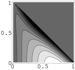
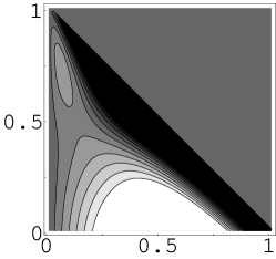
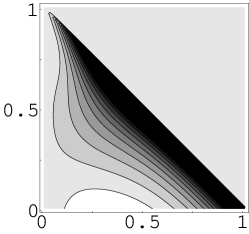
Figure 18: The replica symmetric energy (A.20) as a function of $\rho_{+}$ (vertical axis) and $\rho_{-}$ (horizontal axis), for $p=0.35$, $0.4$ and $0.45$ (from left to right). Notice that only the region $\rho_{+}+\rho_{-}\leq 1$ is meaningful. The energy vanishes as $\rho_{-}\to 0$.

In Fig. 18 we plot $\epsilon(\rho_{+},\rho_{-})$ for three different values of the erasure probability $p_{1}$, $p_{2}$ and $p_{3}$, with $p_{1}<p_{2}<p_{d}<p_{3}$. It is easy to guess the qualitative behavior of $\epsilon(\rho_{+},\rho_{-})$ as $p$ is varied. For small values of $p$ no glassy extremal point with $\rho_{+},\rho_{-}>0$ can be found. At some value $p^{*}<p_{d}$ two such points appear: a maximum and a saddle. At the dynamical threshold $p_{d}$ the saddle point collapses onto the $\rho_{-}=0$ axis.

Figure 19: The energy density (right-hand graph) and the position in the $(\rho_{+},\rho_{-})$ plane of the two non-trivial RS solutions as a function of the erasure probability $p$. The continuous lines refer to the saddle point and the dashed line to the maximum.

This picture can be confirmed by more careful study. The two glassy solutions appear at $p^{*}\approx 0.3844$. In Fig. (19) we report the corresponding energies and their position in the $(\rho_{+},\rho_{-})$ plane as functions of $p$.

Which of the two solutions is the physical one? We argue in favor of the saddle point for the following reasons:

• According to the standard recipe [43], free energy has to be minimized with respect to overlaps involving an odd number of replicas and maximized with respect to overlaps of an even number of replicas. In our case $\rho_{+}-\rho_{-}$ is the magnetization (an odd overlap) and $\rho_{+}+\rho_{-}$ is related to the two replicas overlap. We expect therefore the physical solution to have a stable and an unstable directions.

• Two well-known relatives of our model are the ferromagnet and the $\pm J$ spin glass on random hypergraphs [20, 21]. In this cases a symmetric solution ($\rho_{+}=\rho_{-}$) exists and is accepted to describe the glassy states. When regarded in the full $(\rho_{+},\rho_{-})$ plane this solution appear to be a saddle point in the spin glass model, and to have zero second derivative in the ferromagnetic model.

• One can try to solve Eqs, (A.13)-(A.16) iteratively. This procedure is analogous, within the Ansatz (A.12), to the population dynamics algorithm, which is commonly believed to converge to the correct solution. The iterative procedure converges to the saddle point.

Nonetheless the qualitative picture that one would expect from the behavior of decoding algorithms is quite different from the one offered by the replica symmetric solution. We expect metastable state to appear with positive energy at $p_{d}$ and the minimum among their energies to vanish at $p_{c}$. It is therefore necessary to go beyond the replica symmetric approximation.

A.2 Replica symmetry breaking

The exact computation of the 1RSB free energy is a very difficult task for a finite connectivity model [18]. Good results can be obtained the following variational Ansatz (see Ref. [56] for the general philosophy of the variational approach)

$$\lambda(\vec{\sigma}) = (1-p)\delta_{\vec{\sigma},\vec{\sigma}_{0}}+pf(\underline{\sigma}^{(1)})\cdot\dots\cdot f(\underline{\sigma}^{(n/m)})\,,$$ (A.21)

$$\widehat{\lambda}(\vec{\sigma}) = \widehat{f}(\underline{\sigma}^{(1)})\cdot\dots\cdot\widehat{f}(\underline{\sigma}^{(n/m)})$$ (A.22)

where $\underline{\sigma}^{(\alpha)}=(\sigma^{(\alpha-1)m+1},\dots,\sigma^{\alpha m})$. This amounts to considering a fraction the spins (namely, the ones with an infinite magnetic field) as frozen in the $+1$ state, and assuming all the other spins to be equivalent. In the $n\to 0$ limit we get $\partial_{n}S[\lambda,\widehat{\lambda}]\to\phi[f,\widehat{f}]$ with

$$\phi[f,\widehat{f}] = \frac{\overline{l}p}{m}\log\left(\sum_{\underline{\sigma}}f(\underline{\sigma})\widehat{f}(\underline{\sigma})\right)-\frac{p}{m}\sum_{l=2}^{\infty}v_{l}\log\left(\sum_{\underline{\sigma}}\widehat{f}(\underline{\sigma})^{l}\right)-$$

$$-\frac{\overline{l}}{\overline{k}m}\sum_{\nu=0}^{\infty}g_{\nu}\log\left[\sum_{\underline{\sigma}_{1}\dots\underline{\sigma}_{k}}J^{(m)}_{\beta}(\underline{\sigma}_{1},\dots,\underline{\sigma}_{k})f(\underline{\sigma}_{1})\dots f(\underline{\sigma}_{k})\right]\,,$$

where $\underline{\sigma}$ are $m$-components replicated spins and Notice that the energy (A.2) is invariant under a multiplicative rescaling of $f(\underline{\sigma})$ and $\widehat{f}(\underline{\sigma})$. We shall fix this freedom by requiring that $\sum_{\underline{\sigma}}f(\underline{\sigma})=\sum_{\underline{\sigma}}\widehat{f}(\underline{\sigma})=1$.

Substituting

$$f(\underline{\sigma})\equiv\int\!dx\,\rho(x)\,\frac{e^{\beta x\sum_{a=1}^{m}\sigma^{a}}}{(2\cosh\beta x)^{m}}\,,\;\;\;\;\;\;\;\;\widehat{f}(\underline{\sigma})\equiv\int\!dy\,\hat{\rho}(y)\frac{e^{\beta y\sum_{a=1}^{m}\sigma^{a}}}{(2\cosh\beta y)^{m}}\,,$$ (A.24)

we obtain

$$\beta\phi[\rho,\hat{\rho}] = \frac{\overline{l}p}{m}\log\left[\int\!d\rho(x)d\hat{\rho}(y)\,(1+\tanh\beta x\tanh\beta y)^{m}\right]-\frac{\overline{l}}{\overline{k}}\log\left(\frac{1+e^{-2\beta}}{2}\right)-$$

$$\!\!\!\!-\frac{\overline{l}}{\overline{k}m}\sum_{\nu=0}^{\infty}g_{\nu}\log\left[\int\!\prod_{i=1}^{\nu}d\rho(x_{i})\,(1+\tanh\beta\tanh\beta x_{1}\cdots\tanh\beta x_{\nu})^{m}\right]-$$

$$\!\!\!\!-\frac{p}{m}\sum_{l=2}^{\infty}v_{l}\log\left\{\int\!\prod_{i=1}^{l}d\hat{\rho}(y_{i})\,\left[\prod_{i=1}^{l}(1+\tanh\beta y_{i})+\prod_{i=1}^{l}(1-\tanh\beta y_{i})\right]\right\}\,,$$

and the corresponding saddle point equations:

$$\frac{\rho(x)}{(2\cosh\beta x)^{m}} = \frac{1}{{\mathbb{Z}}\,\overline{l}}\sum_{l=2}^{\infty}v_{l}l\,B_{l}^{-1}\,\int\!\prod_{i=1}^{l-1}\frac{d\hat{\rho}(y_{i})}{(2\cosh\beta y_{i})^{m}}\,\delta(x-\sum_{i=1}^{l-1}y_{i})\,,$$ (A.26)

$$\hat{\rho}(y) = \frac{1}{{\mathbb{Q}}}\sum_{\nu=1}^{\infty}f_{\nu-1}A^{-1}_{\nu}\int\!\prod_{i=1}^{\nu-1}d\rho(y_{i})\,\delta(y-\frac{1}{\beta}{\rm arctanh}[\tanh\beta\tanh\beta y_{1}\cdots\tanh\beta y_{\nu-1})\,,$$

where $f_{\nu-1}\equiv g_{\nu}\nu/(p\overline{k})$, cf. Eq. (A.7), and

$$B_{l} \equiv \int\!\prod_{i=1}^{l}d\hat{\rho}(y_{i})\,\left[\prod_{i=1}^{l}(1+\tanh\beta y_{i})+\prod_{i=1}^{l}(1-\tanh\beta y_{i})\right]^{m}$$ (A.28)

$$A_{\nu} \equiv \int\!\prod_{i=1}^{\nu}d\rho(x_{i})\,[1+\tanh\beta\tanh\beta x_{1}\cdots\tanh\beta x_{\nu}]^{m}\,.$$ (A.29)

The constants ${\mathbb{Z}}$ and ${\mathbb{Q}}$ can be chosen to enforce the normalization condition $\int\!d\rho(x)=\int\!d\hat{\rho}(y)=1$.

In the $\beta\to\infty$ limit, we adopt the Ansatz (A.12) for $\rho(x)$ and $\hat{\rho}(y)$ and keep $m\beta=\mu$ fixed. We obtain the following free energy:

$$\phi(\mu) = \frac{\overline{l}p}{\mu}\log\left\{1+(e^{-2\mu}-1)[\rho_{+}\hat{\rho}_{-}+\rho_{-}\hat{\rho}_{+}]\right\}-$$

$$-\frac{\overline{l}}{\overline{k}\mu}\sum_{\nu=0}^{\infty}g_{\nu}\log\left\{1+\frac{1}{2}(e^{-2\mu}-1)[(\rho_{+}+\rho_{-})^{\nu}-(\rho_{+}-\rho_{-})^{\nu}]\right\}-$$

$$-\frac{p}{\mu}\sum_{l=2}^{\infty}v_{l}\log\left\{\sum_{n_{+},n_{0},n_{-}}\!\!\!\!\!{}^{\prime}\,\frac{l!}{n_{+}!n_{0}!n_{-}!}\hat{\rho}_{+}^{n_{+}}\hat{\rho}_{0}^{n_{0}}\hat{\rho}_{-}^{n_{-}}\,e^{-2\mu\min(n_{+},n_{-})}\right\}\,,$$

the sum $\sum^{\prime}$ being restricted to the integers $n_{+},n_{0},n_{-}\geq 0$ such that $n_{+}+n_{0}+n_{-}=l$. The saddle point equations are

$$\hat{\rho}_{+} = \frac{1}{2{\mathbb{Q}}}\sum_{\nu=1}^{\infty}f_{\nu-1}A_{\nu}^{-1}\,[(\rho_{+}+\rho_{-})^{\nu-1}+(\rho_{+}-\rho_{-})^{\nu-1}]\,,$$ (A.31)

$$\hat{\rho}_{-} = \frac{1}{2{\mathbb{Q}}}\sum_{\nu=1}^{\infty}f_{\nu-1}A_{\nu}^{-1}\,[(\rho_{+}+\rho_{-})^{\nu-1}-(\rho_{+}-\rho_{-})^{\nu-1}]\,,$$ (A.32)

$$\rho_{+} = \frac{1}{{\mathbb{Z}}\,\overline{l}}\sum_{l=2}^{\infty}v_{l}l\,B_{l}^{-1}\!\!\!\!\!\!\sum_{n_{+}>n_{-};\,n_{0}}\frac{(l-1)!}{n_{+}!n_{0}!n_{-}!}\,\hat{\rho}_{+}^{n_{+}}\hat{\rho}_{0}^{n_{0}}\hat{\rho}_{-}^{n_{-}}\ \,e^{-2\mu n_{-}}\,\delta_{n_{+}+n_{0}+n_{-},l-1}\,,$$ (A.33)

$$\rho_{-} = \frac{1}{{\mathbb{Z}}\,\overline{l}}\sum_{l=2}^{\infty}v_{l}l\,B_{l}^{-1}\!\!\!\!\!\!\sum_{n_{-}>n_{+};\,n_{0}}\frac{(l-1)!}{n_{+}!n_{0}!n_{-}!}\,\hat{\rho}_{+}^{n_{+}}\hat{\rho}_{0}^{n_{0}}\hat{\rho}_{-}^{n_{-}}\,e^{-2\mu n_{+}}\,\delta_{n_{+}+n_{0}+n_{-},l-1}\,,$$ (A.34)

where

$$A_{\nu} = 1+\frac{1}{2}(e^{-2\mu}-1)[(\rho_{+}+\rho_{-})^{\nu}-(\rho_{+}-\rho_{-})^{\nu}]\,,$$ (A.35)

$$B_{l} = \sum_{n_{+},n_{0},n_{-}}\frac{l!}{n_{+}!n_{0}!n_{-}!}\hat{\rho}_{+}^{n_{+}}\hat{\rho}_{0}^{n_{0}}\hat{\rho}_{-}^{n_{-}}\,e^{-2\mu\min(n_{+},n_{-})}\,\delta_{n_{+}+n_{0}+n_{-},l}\,,$$ (A.36)

$${\mathbb{Q}} = \sum_{\nu=1}^{\infty}f_{\nu-1}A_{\nu}^{-1}\,,$$ (A.37)

$${\mathbb{Z}} = \frac{1}{\overline{l}}\sum_{l=2}^{\infty}v_{l}l\,B_{l}^{-1}\sum_{n_{+},n_{0},n_{-}}\frac{(l-1)!}{n_{+}!n_{0}!n_{-}!}\,\hat{\rho}_{+}^{n_{+}}\hat{\rho}_{0}^{n_{0}}\hat{\rho}_{-}^{n_{-}}\ \,e^{-2\mu\min(n_{+},n_{-})}\,\delta_{n_{+}+n_{0}+n_{-},l-1}\,.$$ (A.38)

It is interesting to consider some particular asymptotics of the above results. By taking the limit $\mu\to 0$ we recover the replica symmetric energy (A.20) and the saddle point equations (A.13)-(A.16). In the $\mu\to\infty$ limit we have $\phi(\mu)\mu\to\phi_{\infty}(\rho,\hat{\rho})$. Notice that, from Eq. (4.34), we get $\phi_{\infty}(\rho,\hat{\rho})=-\Sigma(0)$, $\Sigma(0)$ being the zero-energy complexity. The explicit expression for this quantity is

$$\phi_{\infty}(\rho,\hat{\rho}) = \overline{l}p\,\log[1-(\rho_{+}\hat{\rho}_{-}+\rho_{-}\hat{\rho}_{+})]-p\sum_{l=2}^{\infty}v_{l}\log\{(1-\hat{\rho}_{+})^{l}+(1-\hat{\rho}_{-})^{l}-\hat{\rho}_{0}^{l}\}-$$ (A.39)

$$-\frac{\overline{l}}{\overline{k}}\sum_{\nu=0}^{\infty}g_{\nu}\log\left\{1-\frac{1}{2}[(\rho_{+}+\rho_{-})^{\nu}-(\rho_{+}-\rho_{-})^{\nu}]\right\}\,,$$

whose minimization yields the following saddle point equations:

$$\hat{\rho}_{+} = \frac{1}{2{\mathbb{Q}}}\sum_{\nu=1}^{\infty}f_{\nu-1}A_{\nu}^{-1}\,[(\rho_{+}+\rho_{-})^{\nu-1}+(\rho_{+}-\rho_{-})^{\nu-1}]\,,$$ (A.40)

$$\hat{\rho}_{-} = \frac{1}{2{\mathbb{Q}}}\sum_{\nu=1}^{\infty}f_{\nu-1}A_{\nu}^{-1}\,[(\rho_{+}+\rho_{-})^{\nu-1}-(\rho_{+}-\rho_{-})^{\nu-1}]\,,$$ (A.41)

$$\rho_{+} = \frac{1}{{\mathbb{Z}}\,\overline{l}}\sum_{l=2}^{\infty}v_{l}l\,B_{l}^{-1}[(1-\hat{\rho}_{-})^{l-1}-(1-\hat{\rho}_{+}-\hat{\rho}_{-})^{l-1}]\,,$$ (A.42)

$$\rho_{-} = \frac{1}{{\mathbb{Z}}\,\overline{l}}\sum_{l=2}^{\infty}v_{l}l\,B_{l}^{-1}[(1-\hat{\rho}_{+})^{l-1}-(1-\hat{\rho}_{+}-\hat{\rho}_{-})^{l-1}]\,,$$ (A.43)

with

$$A_{\nu} = 1-\frac{1}{2}[(\rho_{+}+\rho_{-})^{\nu}-(\rho_{+}-\rho_{-})^{\nu}]\,,$$ (A.44)

$$B_{l} = (1-\hat{\rho}_{+})^{l}+(1-\hat{\rho}_{-})^{l}-(1-\hat{\rho}_{+}-\hat{\rho}_{-})^{l}\,.$$ (A.45)

We look for a solution of Eqs. (A.31)-(A.34) which is the analytic continuation of the “physical” one identified in the previous Section for $\mu=0$. Such a solution exists in some interval $\mu_{1}(p)<\mu<\mu_{2}(p)$. For $p<p^{*}$ no physical solution exists for any value of $\mu$. For $p^{*}<p<p_{d}$, $0=\mu_{1}(p)<\mu_{2}(p)$ and $\phi(\mu)$ is a monotonously increasing function between $\mu_{1}(p)$ and $\mu_{2}(p)$. A physical solution exists but we cannot associate to it any “well-behaved” complexity. Above $p_{d}$ we have $0<\mu_{1}(p)<\mu_{2}(p)=\infty$ and a “well-behaved” complexity can be computed by Legendre-transforming $\mu\phi(\mu)$, cf. Eq. (4.34). The complexity $\Sigma(\epsilon)$ is non-zero between $\epsilon_{s}$ and $\epsilon_{d}$. At $p=p_{c}$ the static energy $\epsilon_{s}$ vanishes: more than one codeword (more precisely, about $\exp\{N\Sigma(0)\}$ codewords) is consistent with the received message.

A.2.1 Beyond the factorized Ansatz

The general one-step replica symmetry breaking order parameter [18] is

$$\lambda(\vec{\sigma})=\int\!\!DQ[\rho]\,\prod_{{\cal G}=1}^{n/m}\left[\int\!\!d\rho(x)\,\frac{e^{\beta x\sum_{a\in{\cal G}}\sigma^{a}}}{(2\cosh\beta x)^{m}}\right]\,,\;\;\;\;\;\widehat{\lambda}(\vec{\sigma})=\int\!\!D\widehat{Q}[\hat{\rho}]\,\prod_{{\cal G}=1}^{n/m}\left[\int\!\!d\hat{\rho}(y)\,\frac{e^{\beta y\sum_{a\in{\cal G}}\sigma^{a}}}{(2\cosh\beta y)^{m}}\right]\,.$$

(A.46)

The saddle point equations for functional order parameters $Q[\rho]$ and $\widehat{Q}[\hat{\rho}]$ are given in the next Section for a general channel, cf. Eqs. (B.3), (B.4).

In the previous Section we used a quasi-factorized Ansatz of the form:

$$Q[\rho]=(1-p)\delta[\rho-\delta_{\infty}]+p\,\delta[\rho-\rho_{0}]\,,\;\;\;\;\widehat{Q}[\hat{\rho}]=\delta[\hat{\rho}-\hat{\rho}_{0}]\,,$$ (A.47)

where $\delta[\cdot]$ is a functional delta function, and $\delta_{\infty}(x)$ is the ordinary Dirac delta centered at $x=+\infty$. This Ansatz does not satisfy the saddle point equations (B.3), (B.4), but yields very good approximate results.

Some exact results (within an 1RSB scheme) can be obtained by writing the general decomposition

$$Q[\rho]=u\,Q_{s}[\rho]+(1-u)\,Q_{a}[\rho]\,,\;\;\;\;\widehat{Q}[\hat{\rho}]=\hat{u}\,\widehat{Q}_{s}[\hat{\rho}]+(1-\hat{u})\,\widehat{Q}_{a}[\hat{\rho}]\,,$$ (A.48)

where $Q_{s}[\rho]$ and $\widehat{Q}_{s}[\hat{\rho}]$ are concentrated on the subspace of symmetric distributions (for which $\rho(x)=\rho(-x)$, $\hat{\rho}(y)=\hat{\rho}(-y)$), while $Q_{a}[\rho]$ and $\widehat{Q}_{a}[\hat{\rho}]$ have zero weight on this subspace. Using this decomposition in Eqs. (B.3), (B.4), we get, for the BEC, a couple of equations for $u$ and $\hat{u}$, which are identical to the replica symmetric ones, cf. Eq. (A.18).

The meaning of this result is clear. For $p>p_{d}$ the system decompose in two parts. There exists a core which the iterative algorithms are unable to decode, and is completely glassy. This part is described by the functionals $Q_{s}[\rho]$ and $\widehat{Q}_{s}[\hat{\rho}]$. The rest of the system (the peripheral region) can be decoded by the belief propagation algorithm and, physically, is strongly magnetized. This corresponds to the functionals $Q_{a}[\rho]$ and $\widehat{Q}_{a}[\hat{\rho}]$ (a more detailed study shows that the asymmetry of $\rho$ and $\hat{\rho}$ is, in this case, typically positive).

Appendix B Calculations: the general channel

In this Appendix we give some details of the replica calculation for a general noisy channel (i.e. for a general distribution $p(h)$ of the random fields). In contrast with the BEC case, cf Eqs. (A.12), the local field distributions do not have a simple form even the zero temperature limit. Therefore our results are mainly based on a numerical solution of the saddle point equations.

B.1 Finite temperature

The one-step replica symmetry breaking Ansatz is given in Eqs. (A.46). Inserting in Eq. (3) and taking the $n\to 0$ limit, we get $S[\lambda,\widehat{\lambda}]=n\phi[Q,\widehat{Q}]+O(n^{2})$, with

$$\phi[Q,\widehat{Q}] = \frac{\overline{l}}{m}\int\!DQ[\rho]\int\!D\widehat{Q}[\hat{\rho}]\,\log\left\{\int\!d\rho(x)\int\!d\hat{\rho}(y)\,[1+t_{\beta}(x)t_{\beta}(y)]^{m}\right\}-$$ (B.1)

$$-\frac{\overline{l}}{\overline{k}m}\sum_{k=3}^{\infty}c_{k}\int\!\prod_{i=1}^{k}DQ[\rho_{i}]\log\left\{\int\!\prod_{i=1}^{k}d\rho_{i}(x_{i})[1+t_{\beta}t_{\beta}(x_{1})\cdots t_{\beta}(x_{k})]^{m}\right\}-$$

$$-\frac{1}{m}\sum_{l=2}^{\infty}v_{l}\int\!\prod_{i=1}^{l}D\widehat{Q}[\hat{\rho}_{i}]\,\left\langle\log\left\{\int\!\prod_{i=1}^{l}d\hat{\rho}_{i}(y_{i}){\mathbb{F}}_{l+1}(\frac{\hat{\zeta}h}{\beta},y_{1},\dots,y_{l})^{m}\right\}\right\rangle_{h}-$$

$$-\langle\log\cosh(\hat{\zeta}h)\rangle_{h}+\frac{\overline{l}}{\overline{k}}\log(1+t_{\beta})\,,$$

where we used the shorthands $t_{\beta}(x)=\tanh(\beta x)$, $t_{\beta}=\tanh(\beta)$, and defined

$${\mathbb{F}}_{n}(y_{1},\dots,y_{n})\equiv\prod_{i=1}^{n}(1+t_{\beta}(y_{i}))+\prod_{i=1}^{n}(1-t_{\beta}(y_{i}))\,.$$ (B.2)

The saddle point equations are

$$Q[\rho] = \frac{1}{\overline{l}}\sum_{l=2}^{\infty}v_{l}l\int\!\!dp(h)\int\!\prod_{i=1}^{l-1}D\widehat{Q}[\hat{\rho}_{i}]\,\,\delta[\rho-\rho^{(l)}_{h}[\hat{\rho}_{1},\dots,\hat{\rho}_{l-1}]]\,,$$ (B.3)

$$\widehat{Q}[\hat{\rho}] = \frac{1}{\overline{k}}\sum_{k=3}^{\infty}c_{k}k\int\!\prod_{i=1}^{k-1}DQ[\rho_{i}]\,\,\delta[\hat{\rho}-\hat{\rho}^{(k)}[\rho_{1},\dots,\rho_{k-1}]]\,,$$ (B.4)

where $\delta[\dots]$ denotes the functional delta function, and the $\rho^{(l)}_{h}[\dots]$, $\hat{\rho}^{(k)}[\dots]$ are defined as follows:

$$\frac{\rho^{(l)}_{h}(x)}{(2\cosh\beta x)^{m}} = \frac{1}{\cal Z}\int\!\prod_{i=1}^{l-1}\frac{d\hat{\rho}_{i}(y_{i})}{(2\cosh\beta y_{i})^{m}}\,\,\,\delta(x-\frac{\hat{\zeta}h}{\beta}-y_{1}-\dots-y_{l-1})\,,$$ (B.5)

$$\hat{\rho}^{(k)}(y) = \int\!\prod_{i=1}^{k-1}d\rho_{i}(x_{i})\,\,\,\delta\left[y-\frac{1}{\beta}\,{\rm arctanh}[t_{\beta}\cdot t_{\beta}(x_{1})\cdots t_{\beta}(x_{k-1})]\right]\,.$$ (B.6)

These equations can be solved numerically using the population dynamics algorithm of Ref. [19]. Some outcomes of this approach are reported in Sec. 5.1.2.

B.1.1 The random linear code limit

An alternative to this numerical approach consists in considering a regular $(k,l)$ code and looking at the $k,l\to\infty$ limit with fixed rate $R=1-l/k$. The leading order results are given in Sec. 5.1.1. Here we give the form of the functional order parameters in this limit.

In the ferromagnetic and paramagnetic phases the order parameter is replica symmetric:

$$Q_{P/F}[\rho]=\int\!d\rho_{P/F}(x)\delta[\rho-\delta_{x}]\,,\;\;\;\;\widehat{Q}_{P/F}[\hat{\rho}]=\int\!d\hat{\rho}_{P/F}(y)\delta[\hat{\rho}-\delta_{y}]\,,$$ (B.7)

where $\delta_{x}$ is a delta function centered in $x$. Moreover we have $\rho_{P}(x)=p(x)$, $\hat{\rho}_{P}(y)=\delta(y)$, and $\rho_{F}(x)=\hat{\rho}_{F}(x)=\delta_{\infty}(x)$. Using these results in Eq. (B.1) we get the paramagnetic and ferromagnetic free energies, Eqs. (5.2), (5.3).

In the spin glass phase the functionals $Q[\rho]$ and $\widehat{Q}[\hat{\rho}]$ are non-trivial, although very simple:

$$Q_{SG}[\rho]=\int\!dp(h)\,\delta[\rho-\rho_{SG}^{(h)}]\,,\;\;\;\;\widehat{Q}_{SG}[\hat{\rho}]=\delta[\hat{\rho}-\hat{\rho}_{SG}]\,,$$ (B.8)

where

$$\rho_{SG}^{(h)}(x) = \frac{1}{Z^{(h)}}\sum_{q=0}^{l-1}C^{(h)}_{q}\delta(x-\hat{\zeta}h/\beta-2q+l-1)\,,$$ (B.9)

$$\hat{\rho}_{SG}(y) = \frac{1}{2}\delta(y-1)+\frac{1}{2}\delta(y+1)\,,$$ (B.10)

and

$$C^{(h)}_{q}=\frac{1}{2^{l-1}}\left(\begin{array}[]{c}l-1\\ q\end{array}\right)[2\cosh(\hat{\zeta}h+\beta(2q-l+1))]^{m}\,.$$ (B.13)

Substituting in Eq. (B.1), we get the spin glass free energy (5.5). Notice that the order parameters (B.9) and (B.10) can be used to compute the first correction to the $k,l\to\infty$ limit. For an example of such a calculation we refer to App. B.2.1.

B.2 Zero temperature

In this Appendix we compute the number of metastable states having a fixed overlap with a random configuration $\underline{\sigma}^{\rm out}$. The dynamical and statical thresholds for the BSC can be deduced from the results of this computation, cf. Sec. 5.2. The generalization to other statistical models for the noisy channel is straightforward (but slightly cumbersome from the point of view of notation).

In order to study the existence of metastable states, we consider the constrained partition function:

$$Z(q;\underline{\sigma}^{\rm out})=\sum_{\underline{\sigma}}e^{-\beta H_{\rm exch}(\underline{\sigma})}\delta(Nq-\sum_{i=1}^{N}\sigma^{\rm out}_{i}\sigma_{i})\,,$$ (B.14)

where the received bits $\sigma^{\rm out}_{i}$ are i.i.d. quenched variables: $\sigma^{\rm out}_{i}=+1$ ($-1$) with probability $1-p$ (respectively $p$). We introduce $m$ “real” weakly coupled replicas of the system:

$$Z_{m}(q;\underline{\sigma}^{\rm out})=\int_{-i\infty}^{+i\infty}\prod_{a=1}^{m}\beta\frac{dh_{a}}{2\pi}\,e^{-Nq\sum_{a}h_{a}}\sum_{\{\underline{\sigma}^{a}\}}e^{-\beta\sum_{a=1}^{m}H_{\rm exch}(\underline{\sigma}^{a})+\beta\sum_{a=1}^{m}\sum_{i=1}^{N}h_{a}\sigma^{\rm out}_{i}\sigma^{a}_{i}}\,.$$ (B.15)

For a general channel we should look at the likelihood rather than at the overlap.

We make the hypothesis of symmetry among the $m$ coupled replicas. In particular we use the same value of the Lagrange multiplier for all of them: $h_{a}=h_{0}/\beta m$. We are therefore led to compute

$$\phi(m;h_{0})=-\lim_{n\to 0}\frac{1}{n}\log\overline{\tilde{Z}_{m}(h_{0};\underline{\sigma}^{\rm out})^{n/m}}\,,$$ (B.16)

where

$$\tilde{Z}_{m}(h_{0};\underline{\sigma}^{\rm out})=\sum_{\{\underline{\sigma}^{a}\}}e^{-\beta\sum_{a=1}^{m}H_{\rm exch}(\underline{\sigma}^{a})+(h_{0}/m)\sum_{a=1}^{m}\sum_{i=1}^{N}\sigma^{\rm out}_{i}\sigma^{a}_{i}}\,.$$ (B.17)

Next we take the zero temperature limit keeping $m\beta=\mu$ fixed. With a slight abuse of notation, we have $m\phi(m;h_{0})\to\mu\phi(\mu;h_{0})$. The entropy of metastable states, cf. Eq. (5.7), is obtained as the Legendre transform of $\mu\phi(\mu;h_{0})$:

$$\Sigma_{p}(\epsilon,q)=\mu\epsilon-h_{0}q-\mu\phi(\mu;h_{0})\,,$$ (B.18)

with $\epsilon=\partial_{\mu}[\mu\phi(\mu;h_{0})]$ and $q=-\partial_{h_{0}}[\mu\phi(\mu;h_{0})]$.

The replica expression for $\phi(\mu;h_{0})$ is easily obtained by taking the zero temperature limit on the results of Sec. B.1. The free energy reads (for sake of simplicity we write it for a regular $(k,l)$ code, the generalization is trivial by making use of Eq. (B.1)):

$$\mu\phi[Q,\widehat{Q}] = l\int\!DQ[\rho]\int\!D\widehat{Q}[\hat{\rho}]\,\log\left\{1+\int\!d\rho(x)\int\!d\hat{\rho}(y)\,\theta(-xy)[e^{-2\mu\min(|x|,|y|)}-1]\right\}-$$ (B.19)

$$-\frac{l}{k}\int\!\prod_{i=1}^{k}DQ[\rho_{i}]\log\left\{1+\int\!\prod_{i=1}^{k}d\rho_{i}(x_{i})\theta(-x_{1}\cdots x_{k})[e^{-2\mu\min(1,|x_{1}|,\dots,|x_{k}|)}-1]\right\}-$$

$$-\int\!\prod_{i=1}^{l}D\widehat{Q}[\hat{\rho}_{i}]\,\sum_{\sigma^{\rm out}}p_{\sigma^{\rm out}}\log\left\{\int\!\prod_{i=1}^{l}d\hat{\rho}_{i}(y_{i})\exp[-2\mu{\mathbb{E}}_{\sigma^{\rm out}}(y_{1}\dots y_{l})]\right\}-$$

$$-h_{0}\,,$$

where $p_{\sigma^{\rm out}}=1-p$ for $\sigma^{\rm out}=+1$, and $p_{\sigma^{\rm out}}=p$ for $\sigma^{\rm out}=-1$ and

$${\mathbb{E}}_{\sigma}(y_{1},\dots,y_{l})=\min\left[\sum_{i:y_{i}\sigma<0}|y_{i}|;\,h_{0}/\mu+\sum_{i:y_{i}\sigma>0}|y_{i}|\right]\,.$$ (B.20)

The saddle point equations become in this limit

$$Q[\rho] = \frac{1}{\overline{l}}\sum_{l=2}^{\infty}v_{l}l\sum_{\sigma^{\rm out}}p_{\sigma^{\rm out}}\int\!\prod_{i=1}^{l-1}D\widehat{Q}[\hat{\rho}_{i}]\,\,\delta[\rho-\rho^{(l)}_{\sigma^{\rm out}}[\hat{\rho}_{1},\dots,\hat{\rho}_{l-1}]]\,,$$ (B.21)

$$\widehat{Q}[\hat{\rho}] = \frac{1}{\overline{k}}\sum_{k=3}^{\infty}c_{k}k\int\!\prod_{i=1}^{k-1}DQ[\rho_{i}]\,\,\delta[\hat{\rho}-\hat{\rho}^{(k)}[\rho_{1},\dots,\rho_{k-1}]]\,.$$ (B.22)

The functionals $\rho^{(l)}_{\sigma^{\rm out}}[\dots]$, $\hat{\rho}^{(k)}[\dots]$ are defined as follows:

$$\rho^{(l)}_{\sigma^{\rm out}}(x) = \frac{1}{\cal Z}\int\!\prod_{i=1}^{l-1}d\hat{\rho}_{i}(y_{i})\,\,\,e^{\mu|x|-\mu\sum_{i}|y_{i}|}\,\,\,\delta(x-(h_{0}/\mu)\sigma^{\rm out}-y_{1}-\dots-y_{l-1})\,,$$ (B.23)

$$\hat{\rho}^{(k)}(y) = \int\!\prod_{i=1}^{k-1}d\rho_{i}(x_{i})\,\,\,\delta\left[y-{\rm sign}(x_{1}\cdots x_{k-1})\min(1,|x_{1}|,\dots,|x_{k-1}|)\right]\,.$$ (B.24)

B.2.1 The random linear code limit

Here we consider the large $k$, $l$ limit for the zero temperature free energy $\phi(\mu;h_{0})$. While the leading order can be obtained through elementary methods, cf. Sec. 5.2.1, the next-to-leading order (which is required for obtaining a non-zero dynamic threshold) must be computed within the replica formalism presented in the previous Section.

We will take advantage of the fact that it is sufficient to know the saddle point order parameters to the leading order, in order to compute the free energy to the next-to-leading order. It is easy to check that, for $k,l\to\infty$ we have

$$Q[\rho]=(1-p)\,\delta[\rho-\rho_{+}]+p\,\delta[\rho-\rho_{-}]\,,\;\;\;\;\widehat{Q}_{SG}[\hat{\rho}]=\delta[\hat{\rho}-\hat{\rho}_{0}]\,,$$ (B.25)

where $\hat{\rho}_{0}(y)=(1/2)\delta(y-1)+(1/2)\delta(y+1)$ and

$$\rho_{\sigma}(x) = \frac{1}{Z_{\sigma}}\sum_{q=0}^{l-1}C^{\sigma}_{q}\delta(x-(h_{0}/\mu)\sigma-2q+l-1)\,,$$ (B.26)

$$C^{\sigma}_{q} = \frac{1}{2^{l-1}}\left(\begin{array}[]{c}l-1\\ q\end{array}\right)\exp\{|-\mu(l-1)+2\mu q+h_{0}\sigma|\}\,.$$ (B.29)

These expressions can be obtained by taking the zero temperature limit of Eqs. (B.8)-(B.13).

Substituting these solutions into Eq. (B.19) we get

$$\mu\phi(\mu;h_{0}) = -(1-R)\log\left(\frac{1+e^{-2\mu}}{2}\right)-\log(1+e^{-2h_{0}})-h_{0}-$$

$$-(1-R)\tanh\mu[(1-2p)\tanh h_{0}]^{k}+f_{l}(\mu)(\cosh\mu)^{-l}+$$

$$+O(\tanh h_{0}^{2k},(\cosh\mu)^{-2l})\,,$$

where we defined

$$f_{l}(\mu)=\left\{\begin{array}[]{ll}2^{-l}\sum_{n=(l+1)/2}^{l}\left(\begin{array}[]{c}l\\ n\end{array}\right)e^{\mu(l-2n)}&\mbox{for $l$ odd,}\\ \\ 2^{-l}\sum_{n=l/2}^{l}\left(\begin{array}[]{c}l\\ n\end{array}\right)e^{\mu(l-2n)}-2^{-l-1}\left(\begin{array}[]{c}l\\ l/2\end{array}\right)&\mbox{for $l$ even.}\end{array}\right.$$ (B.40)

For $l\to\infty$, $f_{l}(\mu)\approx(2\pi\mu^{2})^{-1/2}$. It is easy to check that Legendre transform of the first three terms of Eq. (B.2.1) gives the elementary result (5.16). Subsequent terms give the leading corrections.

B.2.2 A variational calculation

The zero temperature equations simplify in the limit $\mu\to\infty$, corresponding to vanishing exchange energy. In that case, a finite value of $q$ is obtained if the magnetic field $h_{0}$ is kept finite, and it can be proved that the relation $q=\tanh(h_{0})$ holds. In this limit, a direct inspection of the saddle point equations reveals that only the values $\pm(l-1)$ are possible for the cavity fields $x$, and the values $\pm 1$ for the $y$’s. More explicitly, the order parameters $Q[\rho]$ and $\widehat{Q}[\hat{\rho}]$ are supported on distributions of the form

$$\rho(x)=\rho_{+}\delta(x-l+1)+\rho_{-}\delta(x+l-1)\,,\;\;\;\;\;\;\hat{\rho}(y)=\hat{\rho}_{+}\delta(y-1)+\hat{\rho}_{-}\delta(y-1)\,\,.$$ (B.41)

The functional order parameter $\widehat{Q}[\hat{\rho}]$, reduces to the probability distributions of a single number ${\hat{\rho}}_{+}$ representing the probability of $y=+1$.

A simple approximation is obtained by using (B.41) and neglecting the fluctuations of ${\hat{\rho}}_{+}$, in the spirit of the “factorized Ansatz” of [20]. This is exact  for $h_{0}=0$, where our model reduces to the one analyzed in [20]. It can be proved that, for $\mu=\infty$ and $h_{0}\neq 0$, this approximation gives the same result as the $k,l\to\infty$ limit, cf. Sec. 5.2.1. For instance in the case of $(k,l)=(6,5)$ we get $p_{c}^{var}=0.264$ which coincides with the exact result.

The same form for the functional order parameter can also be used as a variational approximation for $\mu$ finite, although in this case it is not justified to assume $y=\pm 1$. In Fig. 20, we indicate the region of the $(p,\epsilon)$ plane such that $\Sigma_{p}(\epsilon,1-2p)>0$, as obtained from this simple approach.

Figure 20: The region of metastability as predicted by the approximated Ansatz (B.41) for the (6,5) code.

References

- [1] O. Dubois, R. Monasson, B. Selman and R. Zecchina (eds.), Theor. Comp. Sci. 265, issue 1-2 (2001).
- [2] J.-P. Bouchaud, L. F. Cugliandolo, J. Kurchan and M. Mézard, in Spin Glasses and Random Fields, A. P. Young ed., (World Scientific, Singapore, 1997)
- [3] A. Barg, in Handbook of Coding Theory, edited by V. S. Pless and W. C. Huffman, (Elsevier Science, Amsterdam, 1998).
- [4] D. A. Spielman, in Lecture Notes in Computer Science 1279, pp. 67-84 (1997).
- [5] T. M. Cover and J. A. Thomas, Elements of Information Theory, (Wiley, New York, 1991).
- [6] A. J. Viterbi and J. K. Omura, Principles of Digital Communication and Coding, (McGraw-Hill, New York, 1979).
- [7] R. G. Gallager Information Theory and Reliable Communication (Wiley, New York, 1968)
- [8] C. E. Shannon, Bell Syst. Tech. J. 27, 379-423, 623-656 (1948)
- [9] N. Sourlas. Nature 339, 693-694 (1989).
- [10] N. Sourlas, in Statistical Mechanics of Neural Networks Lecture Notes in Physics 368, edited by L. Garrido (Springer, New York, 1990).
- [11] N. Sourlas, in From Statistical Physics to Statistical Inference and Back, edited by P. Grassberger and J.-P. Nadal (Kluwer Academic, Dordrecht, 1994).
- [12] P. Ruján, Phys.Rev.Lett. 70, 2968-2971 (1993).
- [13] N. Sourlas. Europhys.Lett. 25, 159-164 (1994).
- [14] C. Berrou, A. Glavieux, and P. Thitimajshima. Proc. 1993 Int. Conf. Comm. 1064-1070.
- [15] R. G. Gallager, Low Density Parity-Check Codes (MIT Press, Cambridge, MA, 1963)
- [16] D. J. .C. MacKay, IEEE Trans. Inform. Theory 45, 399-431 (1999).
- [17] S. M. Aji, G. B. Horn and R. J. McEliece, Proc. 1998 IEEE Intl. Symp. Inform. Theory (Cambridge, MA), p.276.
- [18] R. Monasson, J. Phys. A 31 (1998) 513-529.
- [19] M. Mézard and G. Parisi, Eur. Phys. J. B 20, 217 (2001)
- [20] S. Franz, M. Leone, F. Ricci-Tersenghi, R. Zecchina, Phys. Rev. Lett. 87, 127209 (2001)
- [21] S. Franz, M. Mézard, F. Ricci-Tersenghi, M. Weigt, R. Zecchina, Europhys. Lett. 55 (2001) 465
- [22] J. S. Yedidia, W. T. Freeman, Y. Weiss, in Advances in Neural Information Processing Systems 13, edited by T. K. Leen, T. G. Dietterich, and V. Tresp, (MIT Press, Cambridge, MA, 2001)
- [23] J. S. Yedidia, W. T. Freeman, and Y. Weiss, Understanding Belief Propagation and its Generalizations, 2001. MERL technical report TR 2001-22, available at http://www.merl.com/papers/TR2001-22
- [24] I. Kanter and D. Saad, Phys. Rev. Lett. 83, 2660-2663 (1999).
- [25] R. Vicente, D. Saad and Y. Kabashima, Phys. Rev. E. 60, 5352-5366 (1999).
- [26] I. Kanter and D. Saad, Phys. Rev. E. 61, 2137-2140 (1999).
- [27] A. Montanari and N. Sourlas, Eur. Phys. J. B 18, 107-119 (2000).
- [28] A. Montanari, Eur. Phys. J. B 18, 121-136 (2000).
- [29] Y. Kabashima, T. Murayama and D. Saad, Phys. Rev. Lett. 84, 1355-1358 (2000).
- [30] I. Kanter and D. Saad, Jour. Phys. A. 33, 1675-1681 (2000).
- [31] R. Vicente, D. Saad and Y. Kabashima. Europhys. Lett. 51, 698-704 (2000).
- [32] A. Montanari, Eur. Phys. J. B 23, 121-136 (2001).
- [33] Y. Kabashima, N. Sazuka, K. Nakamura and D. Saad, Tighter Decoding Reliability Bound for Gallager’s Error-Correcting Codes, cond-mat/0010173.
- [34] T. Richardson and R. Urbanke, in Codes, Systems, and Graphical Models, edited by B. Marcus and J. Rosenthal (Springer, New York, 2001).
- [35] R. M. Tanner, IEEE Trans. Infor. Theory, 27, 533-547 (1981).
- [36] G. D. Forney, Jr., IEEE Trans. Inform. Theory, 47 520-548 (2001)
- [37] S.-Y. Chung, G. D. Forney, Jr., T. J. Richardson and R. Urbanke, IEEE Comm. Letters, 5, 58–60 (2001).
- [38] M. G. Luby, M. Mitzenmacher, M. A. Shokrollahi, and D. A. Spielman, IEEE Trans. on Inform. Theory, 47, 569-584 (2001)
- [39] M. G. Luby, M. Mitzenmacher, M. A. Shokrollahi, and D. A. Spielman. IEEE Trans. on Inform. Theory, 47 585-598 (2001)
- [40] J. Pearl, Probabilistic reasoning in intelligent systems: network of plausible inference (Morgan Kaufmann, San Francisco,1988).
- [41] Y. Kabashima and D. Saad, Europhys. Lett. 44, 668-674 (1998).
- [42] T. Richardson and R. Urbanke, IEEE Trans. Inform. Theory, 47, 599–618 (2001).
- [43] M. Mezard, G. Parisi and M. A. Virasoro, Spin Glass Theory and Beyond (World Scientific, Singapore, 1987).
- [44] See, for instance, http://www.digitalfountain.com/technology/index.htm
- [45] C. Di, D. Proietti, E. Telatar, T. Richardson and R. Urbanke, Finite length analysis of low-density parity-check codes, submitted IEEE Trans. on Information Theory, (2001)
- [46] W. H. Press, B. P. Flannery, S. A. Teukolsky, and W. T. Vetterling, Numerical Recipes, (Cambridge University Press, Cambridge, 1986).
- [47] R. Monasson, Phys. Rev. Lett. 75, 2847-2850 (1995)
- [48] S. Franz, G. Parisi, J. Phys. I (France) 5 (1995) 1401
- [49] M. Sipser and D. A. Spielman, IEEE Trans. on Inform. Theory, 42, 1710-1722 (1996).
- [50] S. Kirkpatrick, C.D. Vecchi, and M.P. Gelatt, Science 220, 671 (1983)
- [51] B. Derrida. Phys. Rev. B 24, 2613-2626 (1981).
- [52] A. Cavagna, J. P. Garrahan, and I. Giardina, J. Phys. A, 32, 711 (1999).
- [53] H. Nishimori. J. Phys. C 13, 4071-4076 (1980).
- [54] H. Nishimori. Prog. Theor. Phys. 66, 1169-1181 (1981).
- [55] H. Nishimori and D. Sherrington, Absence of Replica Symmetry Breaking in a Region of the Phase Diagram of the Ising Spin Glass, cond-mat/0008139.
- [56] G. Biroli, R. Monasson, and M. Weigt, Eur. Phys. J. B 14, 551-568 (2000).
- [57] M. Mézard, G. Parisi, and R. Zecchina, in preparation.