[

Chiral phase transitions: focus driven critical behavior in systems with planar and vector ordering

Abstract

The fixed point that governs the critical behavior of magnets described by the $N$-vector chiral model under the physical values of $N$ ($N=2,3$) is shown to be a stable focus both in two and three dimensions. Robust evidence in favor of this conclusion is obtained within the five-loop and six-loop renormalization-group analysis in fixed dimension. The spiral-like approach of the chiral fixed point results in unusual crossover and near-critical regimes that may imitate varying critical exponents seen in physical and computer experiments.

]

The critical behavior of the $N$-vector chiral model remains a controversial issue, being, at the same time, of prime interest for those studying phase transitions in helical magnets, stacked triangular antiferromagnets, and frustrated Josephson-junctions arrays both theoretically and experimentally. In principle, this model should reproduce the main features of phase transitions into chiral states in above substances, but various approaches and approximation schemes still yield quite different theoretical results (see [2, 3, 4] for review and [5, 6, 7, 8, 9, 10, 11, 12, 13, 14, 15, 16] for most recent three- and two-dimensional results). Even within the same, otherwise powerful field-theoretical renormalization-group (RG) approach the theoretical predictions are found to strongly, on the qualitative level, depend on the order of approximation and the reference point of the $\epsilon$-expansion [7, 11, 17, 18, 19, 20]. The experimental data for the critical exponents obtained in several relevant materials turn out also to be considerably scattered (see [2, 3, 4, 7, 21, 22, 23] and references therein).

In this work, we put forward the idea that the controversial situation one faces studying the phase transitions in the aforementioned systems may reflect the quite unusual mode of critical behavior appropriate to the $N$-vector chiral model under the physical values of $N$. To argue this conjecture, we analyze the critical thermodynamics of the two-dimensional and three-dimensional chiral models within the five-loop and six-loop renormalization-group approximations in fixed dimension and determine the structure of RG flows for $N=2,3$. In the course of this study, the advanced resummation technique is used that proved to be effective even near the borderline where the divergent RG series loose their Borel summability [7, 24, 25]. We will show that the critical behavior of the systems with planar and vector chiral ordering is governed by the stable fixed point which is a focus attracting RG trajectories in a spiral-like manner. Approaching the fixed point in a non-monotonic way, looking somewhat irregular, may result in a large variety of crossover and near-critical regimes that give rise to strongly scattered effective critical exponents seen in numerous experiments and computer simulations.

We start with the Landau-Ginzburg-Wilson Hamiltonian of the $D$-dimensional chiral model

$${\cal H}=\int d^{D}x \left\{{1\over 2}\sum_{a}\left[(\partial_{\mu}\phi_{a})^{2}+r\phi_{a}^{2}\right]+{1\over 4!}u_{0}\left(\sum_{a}\phi_{a}^{2}\right)^{2}\right.$$ (2)

$$\left.+{1\over 4!}v_{0}\sum_{a,b}\left[(\phi_{a}\cdot\phi_{b})^{2}-\phi_{a}^{2}\phi_{b}^{2}\right]\right\},$$

where $\phi_{a}$, $a=1,2$ are two $N$-component vectors. Under $v_{0}>0$ this Hamiltonian describes transitions into the phase with noncollinear ordering, i.e. into the chiral state. Since the lower-order renormalization-group approximations failed to give consistent results, we are in a position to study the critical behavior of the model (1) on the base of RG series of maximal length. For the three-dimensional chiral model such record, six-loop series were calculated in [7], while in two dimensions only four-loop RG expansions were known [11]. Aiming to obtain more reliable results, we extend the latter series to the five-loop order, using numerical values of the five-loop integrals evaluated in [26]; explicit expressions for the five-loop contributions to $\beta$-functions and critical exponents will be published elsewhere [27].

The renormalization-group expansions are known to be divergent and some resummation procedure should be applied to extract proper physical predictions and numerical estimates. Taking into account the properties of Borel summability and the large order behavior of the series in two [11] and three [7] dimensions, we resum the perturbative expressions by means of a Borel transformation combined with an appropriate conformal mapping [28] for the analytical extension of the Borel transform. With this resummation procedure we obtain the following approximants for each perturbative series $R({\overline{u}},{\overline{v}})$:

$$E({R})_{p}(\alpha,b;\bar{u},\bar{v}) = \sum_{k=0}^{p}B_{k}(\alpha,b;\bar{v}/\bar{u})$$ (3)

$$\times \int_{0}^{\infty}dt\,t^{b}e^{-t}{y(\bar{u}t;\bar{v}/\bar{u})^{k}\over[1-y(\bar{u}t;\bar{v}/\bar{u})]^{\alpha}}$$ (4)

where

$$y(x;z)={\sqrt{1-x/\overline{u}_{b}(z)}-1\over\sqrt{1-x/\overline{u}_{b}(z)}+1},$$ (5)

and ${\overline{u}}_{b}$ is the singularity of the Borel transform (evaluated in Ref. [7, 11]) closest to the origin at fixed $z={\overline{v}}/{\overline{u}}$. Varying two parameters $\alpha$ and $b$ we are able to estimate the systematic error of the final results. We consider the 18 approximants for each $\beta$ function that minimize the difference between perturbative orders: the approximants with $b=5,7,\dots,15$ and $\alpha=0,1,2$ are used for the two-dimensional models [11], whereas in three dimensions we choose the approximants with $b=3,6\dots,18$ and $\alpha=0,2,4$ [7].

Applying this procedure to the evaluation of the common zeros of the $\beta$ functions, we find in three dimensions a chiral fixed point, as in [7]. In two dimensions the five-loop results also confirm the existence of the chiral fixed point found earlier at the four-loop level [11].

Then we look at the stability properties of these fixed points. Since the exponents $\omega_{+}$ and $\omega_{-}$ determining the fixed point stability are eigenvalues of the matrix

$$\Omega=\left(\matrix{\displaystyle\frac{\partial\beta_{\overline{u}}({\overline{u}},{\overline{v}})}{\partial{\overline{u}}}&\displaystyle\frac{\partial\beta_{\overline{u}}({\overline{u}},{\overline{v}})}{\partial{\overline{v}}}\cr&\cr\displaystyle\frac{\partial\beta_{\overline{v}}({\overline{u}},{\overline{v}})}{\partial{\overline{u}}}&\displaystyle\frac{\partial\beta_{\overline{v}}({\overline{u}},{\overline{v}})}{\partial{\overline{v}}}}\right)\;.$$ (6)

we consider the numerical derivatives of each pair of approximants of the two $\beta$-functions at their common zero. The majority of the eigenvalues, evaluated in two and three dimensions using 324 combinations of the approximants for each case, has non-vanishing imaginary parts. Namely, for $D=2$, $N=2$ the complex eigenvalues are produced by 87% of working approximants, for $D=2$, $N=3$ - by 89%, and for $D=3$, $N=2$ - by 76.5%. For the physically important three-dimensional model with $N=3$, all the approximants employed are found to give the eigenvalues with non-zero imaginary parts. To have reliable numerical estimates for $\omega_{+}$ and $\omega_{-}$, we limit ourselves by the approximants that yield the chiral fixed point coordinates compatible with their final, properly weighted values. The approximates leading to purely real eigenvalues of the stability matrix are discarded in the course of the averaging procedure.

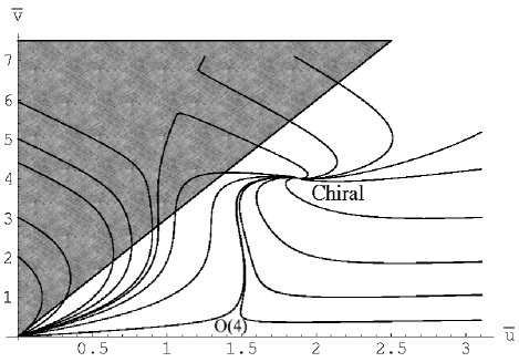
FIG. 1.: RG flow for the physically important case $D=3$, $N=2$. Both $\beta$-functions are represented by the approximants with $\alpha=2$ and $b=6$. With this choice, the chiral fixed point coordinates $({\overline{u}},{\overline{v}})$ are $(1.882,4.017)$.

Thus, for the three-dimensional model with $N=2$ we obtain

$$\omega_{\pm}= 1.40(35)\pm i\,1.00(45), \quad 5\;loop,$$ (7)

$$\omega_{\pm}= 1.70(40)\pm i\,0.90(40), \quad 6\;loop,$$ (8)

while for $N=3$

$$\omega_{\pm}= 0.85(20)\pm i\,0.95(15), \quad 5\;loop,$$ (9)

$$\omega_{\pm}= 1.00(20)\pm i\,0.80(25), \quad 6\;loop,$$ (10)

In two dimensions we have for $N=2$

$$\omega_{\pm}= 1.50(25)\pm i\,1.00(45), \quad 4\;loop,$$ (11)

$$\omega_{\pm}= 2.05(35)\pm i\,0.80(55), \quad 5\;loop,$$ (12)

and for $N=3$

$$\omega_{\pm}= 1.30(25)\pm i\,0.50(35), \quad 4\;loop,$$ (13)

$$\omega_{\pm}= 1.55(25)\pm i\,0.55(35), \quad 5\;loop.$$ (14)

The appearance of imaginary parts comparable in magnitude with the real ones clearly indicates that the chiral critical behavior is controlled by the focus fixed point both in three and two dimensions [29].

To further confirm this conclusion, we apply also the resummation by means of the Padé-Borel-Leroy technique (see e.g. Refs. [4, 26]). The results are substantially equivalent, although the statistics is much less significant due to a large number of defective Padé approximants (i.e. possessing dangerous poles) generated during the resummation.

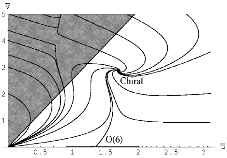
FIG. 2.: RG flow for the physically interesting case $D=3$, $N=3$. Both $\beta$-functions are given by approximants with $\alpha=2$ and $b=9$, the chiral fixed point is located at $(1.702,2.858)$.

In order to substantiate how the focus driven critical behavior manifests itself in the RG flows, we investigated the structure of these flows, given by the resummed five-loop ($2D$) and six-loop ($3D$) RG expansions. Here, we report four examples of RG flows corresponding to physical values of $N$ and generated, for certain values of $D$, by the typical working approximants. They are presented in Figs. 1, 2, 3, and 4, clearly demonstrating the spiral-like approach of the chiral fixed point. Obviously, all the RG flows are quantitatively correct only within the regions where the singularity of the Borel transform closest to the origin is on the real negative axis (see [7, 11]); in Figs. 1, 2, 3, and 4 they correspond to unshaded areas. Nevertheless, we report also the flows in other parts of the coupling constant plane to present a complete qualitative picture [30].

From these figures another peculiar and interesting feature emerges. For some manifold of the starting points, the RG trajectories have the coordinate $v$ that grows very fast at the beginning and seem to reach the region of the first order phase transitions, but just before arriving there these trajectories drastically curve moving toward the stable chiral fixed point. Such RG flows may be considered as a possible explanation of recent Monte Carlo simulations [10] in which a similar behavior was observed (in the space of Binder cumulants), but only up to the first rising up of the coupling $v$, interpreted as an evidence of fluctuation induced first order transition.

Within the context of the results obtained, it is reasonable to discuss the fortune of the unstable anti-chiral fixed point. For almost all the working approximants, this point is seen in the region where the singularity of the Borel transform closest to the origin is on the real positive axis, leaving the existence of the anti-chiral point doubtful. The fact that its location strongly oscillates with varying the approximants indicates that in this domain of $(u,v)$ plane the analysis is not robust. On the other hand, under the presence of the stable focus chiral point, the second, unstable fixed point is not topologically needed on the separatrix dividing the regions of first and second order phase transitions.

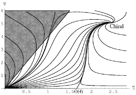
FIG. 3.: RG flow for the two-dimensional model with $N=2$. The approximants used are given by $\alpha=1$ and $b=5$ for $\beta_{\overline{u}}$ and $\alpha=0$ and $b=8$ for $\beta_{\overline{v}}$. In this case, the chiral fixed point is at $(2.427,5.045)$.

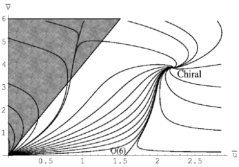
FIG. 4.: RG flow for $D=2$, $N=3$. The approximants used are given by $\alpha=1$ and $b=5$ for $\beta_{\overline{u}}$ and $\alpha=0$ and $b=8$ for $\beta_{\overline{v}}$, the chiral fixed point coordinates are $(2.201,3.854)$.

Finally we report in Fig. 5 the effective exponent $\nu$ for $N=3$ and $d=3$, evaluated along the RG trajectories of Fig. 2. The exponent oscillates within a large range ($0.47\leq\nu\leq 0.72$), even close to the stable fixed point. This provides a possible explanation of the scattered results obtained in simulations and experiments; in fact the majority of numerical results, obtained when a continuous phase transition was observed, are in this wide range.

It is worthy to note that earlier the focus-like stable fixed points were found on the RG flow diagrams of the model describing critical behavior of liquid crystals [31] and of the $O(n)$-symmetric systems undergoing first order phase transition close to the tricritical point [32]. In these cases, however, the independent coupling constants had different scaling dimensionalities and played essentially different roles in forming the critical thermodynamics. Moreover, recently the focus driven chiral phase transition was observed in the three-dimensional model (1) within the three-loop approximation, but for quite unphysical values of $N$ ($N=5,6,7$) [5]. For real physical systems having coupling constants of the same scaling dimensionality, the robust evidence in favor of phase transitions governed by the focus stable fixed point is presented for the first time.

We thank E. Vicari for discussions of the obtained results. The financial support of the Russian Foundation for Basic Research under Grant No. 01-02-17048 (A.I.S.) and the Ministry of Education of Russian Federation under Grant No. E00-3.2-132 (A.I.S.) is gratefully acknowledged. A.I.S. has benefitted from the warm hospitality of Scuola Normale Superiore and Dipartimento di Fisica dell’Università di Pisa, where this research was done.

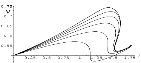
FIG. 5.: Effective exponent $\nu$ for $N=3$ and $d=3$, along RG trajectories. Note that $\nu$ is a multi-valued function of ${\overline{u}}$, as a consequence of the non-monotonic behavior of the RG trajectories.

REFERENCES

- [1] Permanent address
- [2] H. Kawamura, J. Phys.: Condens. Matter 10, 4707 (1998).
- [3] M. F. Collins and O. A. Petrenko, Can. J. Phys. 75, 605 (1997).
- [4] A. Pelissetto and E. Vicari, Phys. Rep. 368, 549 (2002).
- [5] D. Loison, A. I. Sokolov, B. Delamotte, S. A. Antonenko, K. D. Schotte, and H. T. Diep, JETP Letters 72, 337 (2000).
- [6] M. Tissier, B. Delamotte and D. Mouhanna, Phys. Rev. Lett. 84, 5208 (2000); Phys. Rev. B 61, 15327 (2000).
- [7] A. Pelissetto, P. Rossi, and E. Vicari, Phys. Rev. B 63, 140414(R) (2001).
- [8] A. Pelissetto, P. Rossi, and E. Vicari, Nucl. Phys. B 607, 605 (2001).
- [9] A. Pelissetto, P. Rossi, and E. Vicari, Phys. Rev. B 65, 020403(R) (2002).
- [10] M. Itakura, cond-mat/0110306 (unpublished).
- [11] P. Calabrese and P. Parruccini, Phys. Rev. B 64, 184408 (2001).
- [12] G. Ramirez-Santiago and J. V. José, Phys. Rev. Lett. 68, 1224 (1992); Phys. Rev. 49, 9567 (1994); Phys. Rev. Lett. 77, 4849 (1996).
- [13] P. Olsson, Phys. Rev. Lett. 75, 2758 (1995); Phys. Rev. Lett. 77, 4850 (1996); Phys. Rev. B 55, 3585 (1997).
- [14] V. I. Marconi and D. Domínguez, Phys. Rev. Lett. 87, 017004 (2001).
- [15] G. Franzese, V. Cataudella, S. E. Korshunov and R. Fazio, Phys. Rev. B 62, R9287 (2000).
- [16] W. Stephan and B. W. Southern, Phys. Rev. B 61, 11514 (1999); to appear Can. J. Phys., e-print cond-mat/0009115.
- [17] H. Kawamura, Phys. Rev. B 38, 4916 (1988); erratum B 42, 2610 (1990).
- [18] P. Azaria, B. Delamotte and T. Jolicoeur, Phys. Rev. Lett. 64, 3175 (1990).
- [19] S. A. Antonenko and A. I. Sokolov, Phys. Rev. B 49, 15901 (1994).
- [20] S. A. Antonenko, A. I. Sokolov, and K. B. Varnashev, Phys. Lett. A 208, 161 (1995).
- [21] V. P. Plakhty, J. Kulda, D. Visser, E. V. Moskvin, and J. Woznitza, Phys. Rev. Lett. 85, 3942 (2000).
- [22] V. P. Plakhty, W. Schweika, Th. Brückel, J. Kulda, S. V. Gavrilov, L.-P. Regnault, and D. Visser, Phys. Rev. B 64, 100402(R) (2001).
- [23] M. Fiebig, C. Degenhart, and R. V. Pisarev, Phys. Rev. Lett. 88, 027203 (2002).
- [24] J. M. Carmona, A. Pelissetto, and E. Vicari, Phys. Rev. B 61, 15136 (2000).
- [25] A. Pelissetto and E. Vicari, Phys. Rev. B 62, 6393 (2000).
- [26] E. V. Orlov and A. I. Sokolov, Fiz. Tverd. Tela 42, 2087 (2000) [Phys. Solid State 42, 2151 (2000)] and unpublished.
- [27] P. Calabrese, E. V. Orlov, P. Parruccini, and A. I. Sokolov, cond-mat/0207187.
- [28] J. C. Le Guillou and J. Zinn-Justin, Phys. Rev. Lett. 39, 95 (1977); Phys. Rev. B 21, 3976 (1980).
- [29] Big values of the imaginary parts found not only for three-dimensional, but also for two-dimensional systems make us sure that this result is not an artifact of the perturbative analysis and an account for nonanalytic contributions, clearly visible in two dimensions [26], will not kill it. See P. Calabrese, M. Caselle, A. Celi, A. Pelissetto, and E. Vicari, J. Phys A 33, 8155, (2000) and references therein for an explanation of the effects of nonanalyticities in the models.
- [30] We adopt here different rescalings for the four-point renormalized couplings in two and three dimensions; they coincide with those used in Refs. [11] and [7], respectively. Due to this difference, the shaded areas turns out to depend on the space dimensionality . In these pictures the mean-field domain of first-order phase transitions are exactly two times larger than the shaded areas ( in the symmetric normalization of Ref. [11]). Note that saying ”the domain of the first-order phase transitions” we mean, as usually, the region where the quartic form in free energy expansion can acquire negative values. In fact, because of the presence of the higher-order terms in this expansion that make the system globally stable at any temperature, the true domains of the first-order transitions may be substantially more narrow than those predicted by the mean-field approximation.
- [31] A. L. Korzhenevskii and B. N. Shalaev, Zh. Eksp. Teor. Fiz. 76, 2166 (1979) [Sov. Phys. JETP 49, 1094 (1979)].
- [32] A. I. Sokolov, Zh. Eksp. Teor. Fiz. 77, 1598 (1979) [Sov. Phys. JETP 50, 802 (1979)].