Phase Transition in a Random Fragmentation Problem with Applications to Computer Science

Abstract

We study a fragmentation problem where an initial object of size $x$ is broken into $m$ random pieces provided $x>x_{0}$ where $x_{0}$ is an atomic cut-off. Subsequently the fragmentation process continues for each of those daughter pieces whose sizes are bigger than $x_{0}$. The process stops when all the fragments have sizes smaller than $x_{0}$. We show that the fluctuation of the total number of splitting events, characterized by the variance, generically undergoes a nontrivial phase transition as one tunes the branching number $m$ through a critical value $m=m_{c}$. For $m<m_{c}$, the fluctuations are Gaussian where as for $m>m_{c}$ they are anomalously large and non-Gaussian. We apply this general result to analyze two different search algorithms in computer science.

PACS numbers: 02.50.-r, 05.40.-a, 89.20.-a 22 April 2002

Fragmentation is a widely studied phenomena[1] with applications ranging from conventional fracture of solids[2] and collision induced fragmentation in atomic nuclei/aggregates[3] to seemingly unrelated fields such as disordered systems[4] and geology[5]. In this paper we consider a problem where an object of initial size (or length) $x$ is first broken into $m$ random pieces of sizes $x_{i}=r_{i}x$ with $\sum_{i=1}^{m}r_{i}=1$ provided the initial size $x>x_{0}$ where $x_{0}$ is a fixed ‘atomic’ threshold. At the next stage, each of those $m$ pieces with sizes bigger than $x_{0}$ is further broken into $m$ random pieces and so on. Clearly the process stops after a finite number of fragmentation or splitting events when the sizes of all the pieces become less than $x_{0}$. This problem and its close cousins have already appeared in numerous contexts including the energy cascades in turbulence[6], rupture processes in earthquakes[7], stock market crashes[8], binary search algorithms[9, 10, 11], stochastic fragmentation[12] and DNA segmentation algorithms[13]. It therefore comes as somewhat of a surprise that there is a nontrivial phase transition in this problem as one tunes the branching number $m$ through a critical value $m=m_{c}$.

In this Letter we study analytically the statistics of the total number of fragmentation events $n(x)$ up till the end of the process as a function of the initial size $x$. We show that, while the average number of events $\mu(x)$ always grows linearly with $x$ for large $x$, the asymptotic behavior of the variance $\nu(x)$, characterizing the fluctuations, undergoes a phase transition at a critical value $m=m_{c}$,

$$\nu(x)\sim\cases{x&$m<m_{c}$,\cr x^{2\theta}&$m\geq m_{c}$\cr}.$$ (1)

The exponent $\theta$ is nontrivial and increases monotonically with $m$ for $m\geq m_{c}$ starting at $\theta(m=m_{c})=1/2$ and the amplitude of the leading $x^{2\theta}$ term has log-periodic oscillations for $m\geq m_{c}$. This signals unusually large fluctuations in $n(x)$ for $m>m_{c}$. The full distribution of $n(x)$ also changes from being Gaussian for $m<m_{c}$ to non-Gaussian for $m>m_{c}$. This phase transition is rather generic for any fragmentation problem with an ‘atomic’ threshold. However the critical value $m_{c}$ and the exponent $\theta$ are nonuniversal and depend on the distribution function of the random fractions $r_{i}$’s. In this Letter we establish this generic phase transition and then calculate explicitly $m_{c}$ and $\theta$ for two special cases with direct applications in computer science.

In this fragmentation problem with a fixed lower cut-off $x_{0}$, one first breaks the initial piece of length $x$ provided $x>x_{0}$ into $m$ pieces of sizes $x_{i}=r_{i}x$. The sizes of each of these ‘daughters’ are then examined. Only those pieces whose sizes exceed $x_{0}$ are considered ‘active’ and those with sizes less than $x_{0}$ are considered ‘frozen’. Each of the active pieces is then subsequently broken into $m$ pieces and so on. The fractions $r_{i}$’s characterizing a splitting event are considered to be independent from one event to another but are drawn each time from the same joint distribution function $\eta_{m}(r_{1},r_{2},\ldots r_{m})$. As the splitting process conserves the total size, the fractions $r_{i}$’s satisfy the constraint $\sum_{i=1}^{m}r_{i}=1$. In addition, we consider the splitting process to be isotropic, i.e., all the $m$ daughters resulting from a splitting event are statistically equivalent. This indicates that the marginal distribution of any one of the $r_{i}$’s is independent of $i$ and is given by,

$$\eta_{1}(r)=\int\ \eta_{m}(r,r_{2},\cdots r_{m})\prod_{i=2}^{m}dr_{i}.$$ (2)

We will henceforth denote the average over the whole history of the splitting procedure (till the end of the process) as ${\overline{\cdots}}$ and the average over the $r_{i}$’s associated with a single splitting event as $\langle\cdot\rangle$. The conservation law along with the isotropy implies that $\langle r\rangle=\int\eta_{1}(r)r\ dr=1/m$.

Clearly the total number of splitting events $n(x)=0$ if $x<x_{0}$. On the other hand if $x>x_{0}$ there will be at least one splitting and it is easy to write a recursion relation for $n(x)$,

$$n(x)=1+\sum_{i=1}^{m}n(r_{i}x).$$ (3)

Using the isotropy of the splitting distribution and taking the average over Eq. (3), we find that $\mu(x)\equiv\overline{n(x)}$ satisfies the recursion for $x>x_{0}$,

$$\mu(x)=1+m\langle\mu(rx)\rangle=1+m\int_{x_{0}/x}^{1}dr\ \eta_{1}(r)\mu(rx),$$ (4)

where the lower limit in the above integral comes from the condition $n(x)=0$ for $x<x_{0}$. Without any loss of generality we set $x_{0}=1$, i.e., we measure all sizes in units of the atomic size. Since $1\leq x<\infty$ in Eq. (4), it is convenient to make a change of variable $x=e^{\alpha}$ so that $0\leq\alpha<\infty$ and write $\mu(e^{\alpha})=F(\alpha)$. The resulting equation for $F(\alpha)$ is solved by taking the Laplace transform of Eq. (4) and one finds that ${\tilde{F}}(s)=\int_{0}^{\infty}d\alpha\ F(\alpha)e^{-s\alpha}$ is given by

$${\tilde{F}}(s)={1\over s\left[1-mw(s)\right]},$$ (5)

where $w(s)=\langle r^{s}\rangle=\int_{0}^{1}dr\ \eta_{1}(r)\ r^{s}$. Assuming ${\tilde{F}}(s)$ has simple poles at $s=\lambda_{k}$, the Laplace transform in Eq. (5) can be inverted to obtain $\mu(x)=a_{0}+\sum_{k}a_{k}x^{\lambda_{k}}$ with $a_{0}=1/(1-m)$ (coming from the pole at $s=0$) and $a_{k}=-1/[m\lambda_{k}w^{\prime}(\lambda_{k})]$. From the conservation law $\langle r\rangle=1/m$, one finds that $s=1$ is always a pole of ${\tilde{F}}(s)$. Besides, since $0\leq r\leq 1$, the pole at $s=1$ is also the one with the largest real part and hence will dominate the large $x$ behavior of $\mu(x)$. Let $\lambda$ and $\lambda^{*}$ denote the pair of complex conjugate poles with the next largest real part. Then keeping only the leading corrections to the asymptotic behavior one finds

$$\mu(x)\approx a_{1}x+a_{2}x^{\lambda}+a_{2}^{*}x^{\lambda^{*}},$$ (6)

where $a_{1}=-1/[mw^{\prime}(1)]=-1/[m\int_{0}^{1}dr\ \eta_{1}(r)r\ln(r)]$.

We now turn to the variance $\nu(x)$ of the total number of splittings $n(x)$:

$$\nu(x)=\overline{\left(n(x)-\mu(x)\right)^{2}}.$$ (7)

By squaring Eq. (3) and after some straightforward algebra we find the recursion relation

$$\nu(x)=f(x)+m\int_{1/x}^{1}dr\ \eta_{1}(r)\nu(rx),$$ (8)

where $f(x)=\langle\left(\sum_{i=1}^{m}\left[\mu(r_{i}x)-\langle\mu(rx)\rangle\right]\right)^{2}\rangle$. Once again the change of variable $x=e^{\alpha}$ followed by a subsequent Laplace transform with respect to $\alpha$, ${\tilde{\nu}}(s)=\int_{0}^{\infty}d{\alpha}\nu(e^{\alpha})e^{-s\alpha}$ yields,

$$\tilde{\nu}(s)={\tilde{f}(s)\over s\left[1-mw(s)\right]}.$$ (9)

Using the asymptotic expression of $\mu(x)$ from Eq. (6) in the expression for $f(x)$ one finds that the leading term of $f(x)$ for large $x$ is given by

$$f(x)\approx b_{1}x^{2\lambda}+b_{2}x^{2\lambda^{*}}+b_{3}x^{(\lambda+\lambda^{*})},$$ (10)

where the $b_{j}$’s are constants. These behaviors indicate that ${\tilde{f}}(s)$ has poles at $s=2\lambda$, $s=2\lambda^{*}$ and $s=\lambda+\lambda^{*}$. Thus when $Re(\lambda)<1/2$, these poles occur to the left of $s=1$ in the complex $s$ plane. From Eq. (9) it follows that the asymptotic large $x$ behavior of $\nu(x)$ will then be controlled by the $s=1$ pole arising from the denominator $\left[1-mw(s)\right]$ and $\nu(x)\sim x$ for large $x$. On the other hand when $Re(\lambda)>1/2$, the dominant poles governing the large $x$ behavior are the three poles of ${\tilde{f}}(s)$ with real part $2Re(\lambda)>1$. Hence in that case, $\nu(x)\sim x^{2\theta}$ where $\theta=Re(\lambda)$. Note also that for $Re(\lambda)\geq 1/2$, the amplitude of the leading term $x^{2\theta}$ in $\nu(x)$ will have log-periodic oscillations due to the nonzero imaginary parts of the poles $\lambda$ and $\lambda^{*}$. This phase transition will always occur whenever one can tune the pole $\lambda$ continuously through the critical value $Re(\lambda)=1/2$. In the following two examples we show explicitly that this can be achieved, in a natural way, by tuning the branching number $m$.

FIG. 1.: Top: The construction of the 3-ary tree for a sequence of numbers between 1 and 10. Bottom: The induced random interval splitting. The nodes and corresponding splittings are labelled a,b,c,d,e and f. An interval can only split if it contains a $\bullet$.

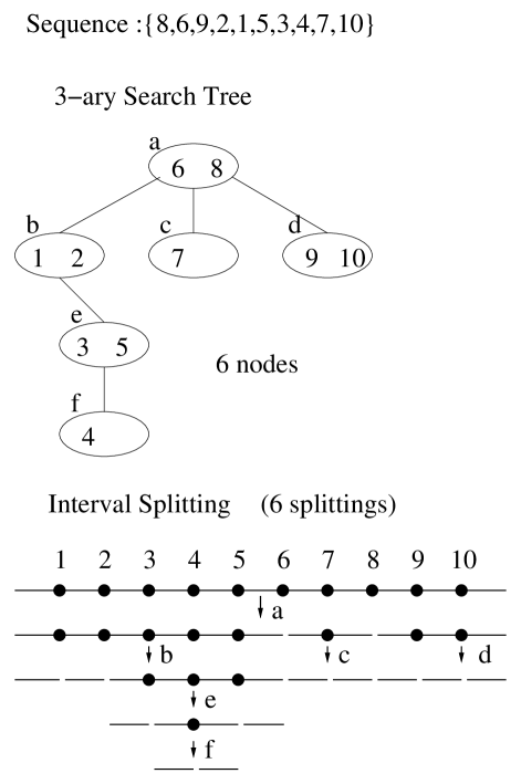
The m-ary search tree: It is well known that one of the most efficient ways to sort the incoming data to a computer is to organize the data on a tree[14]. Consider the sorting of an incoming data string consisting of $N$ distinct elements labelled by the sequence $1,\ 2,\ \cdots N$. Consider a particular random sequence of arrival of these $N$ elements (see Fig. 1). An m-ary search tree stores this sequence on a growing tree structure where each node of the tree can contain at most $(m-1)$ data points[9, 11]. A node if filled branches into $m$ leaves. The first $(m-1)$ elements are stored in the root of the tree in an ordered sequence $w_{1}<w_{2}\cdots<w_{m-1}$. Any subsequent element must belong to one of $m$ sets of numbers $A_{1}=[1,w_{1})$, $A_{i}=(w_{i},w_{i+1})$ with $1\leq i\leq m-2$ and $A_{m}=(w_{m-1},N]$. Associated with each of these sets or intervals we associate a leaf of the tree leading to a new node. A new data point $w$, arriving subsequently, is sent down the leaf corresponding to the set $A_{i}$ if $w\in A_{i}$ and is stored in a daughter node at the base of that leaf. Once a daughter node is filled with $m-1$ numbers it in turn gives rise to $m$ new leaves and so on. An example for a 3-ary search tree with $N=10$ is shown in Fig. (1).

Each sequence of the incoming data will give rise to a different $m$-ary tree configuration. If the incoming data is random, all the trees occur with equal probability. It is easy to see that the total number of occupied nodes $M$ (each containing at least one element) is a random variable as it varies from one tree configuration to another, except for $m=2$ where $M=N$. The statistics of $M$ was recently studied by computer scientists using rather involved combinatorial analysis and it was found that while ${\overline{M}}\sim N$ for large $N$, the variance $\nu\sim N$ for $m<26$ and as $\sim N^{2\theta}$ for $m>26$[15]. We show below that this strange result is just a special case of the general phase transition in the fragmentation problem discussed here.

The construction of the $m$-ary search tree can be mapped exactly onto the splitting of the interval $[1,N]$ [9, 11]. It is easy to see that the incoming elements $w_{1},\ w_{2}\cdots w_{m-1}$ split the initial interval into $m$ parts $A_{i}$. If all the $N!$ possible sequences arrive with equal probability then the points $w_{1},\ w_{2}\cdots w_{m-1}$ are distributed uniformly on $[1,N]$ (these are the numbers stored in the first node). We split the interval $[1,N]$ into $m$ subintervals corresponding to the $A_{i}$’s introduced above. If a subinterval $A_{i}$ is empty (i.e. has no $\bullet$ in Fig. (2)) then no data points can go down the corresponding leaf and hence such an interval (of length $<2$) will not split any further. If the subset $A_{i}$ contains only one $\bullet$, the arrival of the corresponding single data point still splits the interval into $m$ parts (some of the intervals so created may be of length 0). This corresponds to the atomic threshold $x_{0}=2$ in our general problem and $x=N/2$ corresponds to the initial size in units of the atomic size.

The crucial point is that the number of occupied nodes $M$ in the $m$-ary search tree is identical to the number of splittings $n(x=N/2)$ in this fragmentation problem. For large $N$ one can pass to a continuum limit and use the known marginal probability density function $\eta_{1}(r)=(m-1)(1-r)^{m-2}$[10, 11] for the continuum interval splitting problem in our general formula. We get ${\overline{M}}=\mu(x=N/2)\approx{a_{1}N}/2$ for large $N$ where $a_{1}=1/[{\sum_{k=2}^{m}}1/k]$. Also $w(s)=\langle r^{s}\rangle=(m-1)B(s+1,m-1)$ where $B(m,n)$ is the standard Beta function. Therefore the poles of ${\tilde{F}}(s)$ in Eq. (5) occur at the roots of the equation $m(m-1)B(s+1,m-1)=1$. It is easy to check using Mathematica that one can arrive at the critical condition $Re(\lambda)=1/2$ by tuning $m$ through the value $m=m_{c}\approx 26.0461\cdots$. Therefore, from our general theory, we find that the variance $\nu\sim N$ for $m<m_{c}$ and $\nu\sim N^{2\theta}$ for $m>m_{c}$. The exponent $\theta=Re(\lambda)$ where $\lambda$ is the root of $m(m-1)B(s+1,m-1)=1$ that is closest (to the left) to $s=1$ when $m>m_{c}$.

FIG. 2.: An example of the splitting of a rectangle into four daughter rectangles about the point ${\bf w}=[l_{1}u_{1},l_{2}u_{2}]$. The same process is continued on each daughter until the area of the daughter becomes less than $x_{0}$.

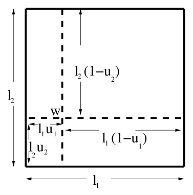
Cuboid Splitting: In the previous problem we have considered the sorting of a data string where each element is a scalar. A natural generalization is when each element is a $D$-dimensional vector ${\bf w}$ whose $k$-th component $w_{k}\in[0,l_{k}]$ for $1\leq k\leq D$. The first element of the data string is then assigned to the point ${\bf w}$ in the cuboid of edge lengths $l_{k}$. If the first element is random, then its components $w_{k}=u_{k}l_{k}$, where the $u_{k}$ are independent random variables uniformly distributed on $[0,1]$. Once this first element is stored, it splits the original cuboid into $2^{D}$ sub-cuboids obtained by drawing $D$ lines perpendicular to each of the faces of the cuboid (see Fig. 2). When the second vector arrives, one compares its components with that of the first element and places it in one of the $2^{D}$ sub-cuboids (and thereby splits that sub-cuboid) and the process continues. After each splitting event, the dimensions of the $m=2^{D}$ new sub-cuboids can be represented by $l^{\prime}_{k}(\sigma)=l_{k}u_{k}(1+\sigma_{k})/2+l_{k}(1-u_{k})(1-\sigma_{k})/2$, where the $\sigma_{k}$ are Ising spins. An example with $D=2$ is shown in Fig(2).

The volume of any of the sub-cuboids upon splitting the cuboid of volume $x$ is $x^{\prime}=xr(\sigma)$, where $r(\sigma)=\prod_{k=1}^{D}\left(u_{k}(1+\sigma_{k})/2+(1-u_{k})(1-\sigma_{k})/2\right)$. Hence in this problem one has $m=2^{D}$ and the marginal distribution of a given $r(\sigma)$ can be shown to be

$$\eta_{1}(r)={[-\ln(r)]^{D-1}\over(D-1)!},\ \ \ 0\leq r\leq 1.$$ (11)

From Eq.(5) with this marginal distribution one finds that

$${\tilde{F}}(s)={1\over{s\left(1-{2^{D}\over(s+1)^{D}}\right)}}.$$ (12)

One then finds $\mu(x)\approx 2x/D$ for large $x$. The function ${\tilde{F}}(s)$ has a total of $(D+1)$ poles: one at $s=0$ and the others at $s=-1+2e^{2\pi in/D}$ with $n=0,1,\ldots(D-1)$. The poles closest to the left of $s=1$ are the complex conjugate pair $\lambda=-1+2e^{2\pi i/D}$ and $\lambda^{*}=-1+2e^{-2\pi i/D}$. Thus $Re(\lambda)=-1+2\cos(2\pi/D)$. From our general theory, it follows that by tuning $m$ or equivalently $D$, it is possible to encounter the critical point $Re(\lambda)=1/2$ at $D=D_{c}=\pi/\sin^{-1}(1/2\sqrt{2})=8.69\ldots$. Hence the variance $\nu(x)\sim x$ for $D<D_{c}$, and for $D\geq D_{c}$, $\nu(x)\sim x^{2\theta}$ where $\theta=Re(\lambda)=2\cos(2\pi/D)-1$.

We have verified the above predictions by numerically carrying out the splitting procedure on a large number of samples with atomic cut-off $x_{0}=1$. The analytical predictions for the mean and the variance are well verified though an accurate measurement of the exponent $\theta$ is difficult due to statistical fluctuations and finite size corrections. We have also measured the histogram of the number of splittings. For $D<D_{c}$ this distribution is Gaussian, however for $D>D_{c}$ the distribution becomes skewed towards large values of $n(x)$ having an anomalous tail. Shown in Fig. (3) is the distribution measured for $D=8$ and $D=10$. The difference is clearly visible. The non-Gaussian behavior is also visible for the case $D=9$ but less pronounced as $Re(\lambda)$ is quite close to $1/2$. While we can rigorously prove that the distribution is indeed Gaussian in the sub-critical regime, we have not been able to calculate the full distribution in the supercritical regime. Qualitatively it is clear however that as $D$ increases the volume of the cuboid becomes more concentrated about its surface and hence the splitting point ${\bf w}$ for large $D$ is generically closer to the surfaces. This means that the splitting procedure will tend to cut the cuboid into more unequal pieces than at lower dimensions, a mixture of blocks of larger volume and slices of smaller volume. It is thus the blocks which are sliced rather than split in their middle which contribute to the long tail in the distribution of $n(x)$.

FIG. 3.: The distribution $p(n(x))$ of the number of splittings of a cuboid of original volume $x=1000$ for $D=8$ (filled circles) and for $D=10$ (filled squares). The distribution is Gaussian for $D=8$, but has a non-Gaussian skewness for $D=10$. The histogram was formed by numerically splitting $5\times 10^{5}$ samples in each case.

In conclusion we have shown that a fragmentation process with an atomic threshold can undergo a nontrivial phase transition in the fluctuations of the number of splittings at a critical value of the branching number $m$. The calculation of the full probability distribution of the number of splittings remains a challenging unsolved problem. We have provided applications of our general results in two computer science problems. The mechanism of this transition is remarkably simple and therefore one expects it to be rather generic with broad applications since many random processes can be mapped to the type of fragmentation model considered here.

REFERENCES

- [1] For a general review of fragmentation, see S. Redner, in Statistical Models for the Fracture of Disordered Media, ed. H.J. Herrmann and S. Roux (Elsevier Science, New York, 1990).
- [2] B.R. Lawn and T.R. Wilshaw, Fracture of Brittle Solids (Cambridge University Press, Cambridge, 1975).
- [3] X. Campi, H. Krivine, N. Sator and E. Plagnol, Eur. Phys. J. D 11, 233 (2000).
- [4] B. Derrida and H. Flyvbjerg, J. Phys. A 20, 5273 (1987); H. Flyvbjerg and N.J. Kjaer, J. Phys. A 21, 1695 (1988); P.G. Higgs, Phys. Rev E 51, 95 (1995); B. Derrida and B. Jung-Muller, J. Stat. Phys. 94, 277 (1999).
- [5] D.L. Turcotte, J. Geophys. Res. 91, 1921 (1986).
- [6] M. Greiner, H.C. Eggers and P. Lipa, Phys. Rev. Lett. 80, 5333 (1998).
- [7] W.I. Newman and A.M. Gabrielov, Int. J. Fract. 50 1, (1991); W.I. Newman and A.M. Gabrielov, T.A. Durand, S.L. Phoenix and D.L. Turcotte, Physica 77D, 200, (1994).
- [8] D. Sornette and A. Johansen, Physica 261A, 581 (1998).
- [9] L. Devroye, J. ACM 33, 489 (1986).
- [10] P.L. Krapivsky and S.N. Majumdar, Phys. Rev. Lett. 85 , 5492 (2000).
- [11] S.N. Majumdar and P.L. Krapivsky, Phys. Rev. E, 65, 036127 (2002).
- [12] P.L. Krapivsky, E. Ben-Naim, and I. Grosse, cond-mat/0108547.
- [13] P. Bernaola-Galván, R. Román-Roldán and J.L. Oliver, Phys. Rev. E 53, 5181 (1996); W. Li, Phys. Rev. Lett. 86, 5815 (2001).
- [14] D.E. Knuth, The Art if Computer Programming, Sorting and Searching, 2nd ed. (Addison-Wesley, Reading, MA, 1988), Vol 3.
- [15] H.M. Mahmoud and B. Pittel, Journal of Algorithms, 10, 52 (1989); H-H. Chern and H-K. Hwang, Random Struct. Alg., 19, 316 (2001).