Vortex transport and voltage noise in disordered superconductors

Abstract

We study, by means of three-dimensional Monte Carlo simulations, the current-voltage (IV) characteristics and the voltage noise spectrum at low temperatures of driven magnetic flux lines interacting with randomly placed point or columnar defects, as well as with periodically arranged linear pinning centers. Near the depinning current $J_{c}$, the voltage noise spectrum $S(\omega)$ universally follows a $1/\omega^{\alpha}$ power law. For currents $J>J_{c}$, distinct peaks appear in $S(\omega)$ which are considerably more pronounced for extended as compared to point defects, and reflect the spatial distribution of the correlated pinning centers.

, , and

The dynamics of flux lines in the mixed state of high-$T_{c}$ superconductors has been a topic of intense interest in the past few years [1]. The area of research is motivated both by important technological questions and a quest of understanding complex non-equilibrium behavior of driven systems. Defects in the superconducting materials can either be localized (point pinning centers, such as oxygen vacancies) or extended. For example, artificial columnar pins are introduced via high-energy ion irradiation to pin the magnetic vortices in order to reduce energy loss due to dissipation when current is passed through the sample [1]. The non-equilibrium dynamics of flux lines in the presence of defects generates non-trivial steady states which can be probed in experiments measuring, e.g., the current-voltage (IV) characteristics [1], the voltage noise power spectrum [2, 3, 4], or local flux density noise [3]. Analytical studies of the vortex dynamics are usually limited to asymptotic regimes [1, 5, 6] when the current $J$ is either much smaller or much larger than the critical current $J_{c}$. The intermediate current regime has been investigated by numerical techniques such as Langevin molecular dynamics simulations [7, 8, 9, 10] or Monte Carlo techniques [11, 12]. These numerical simulations are largely restricted to two dimensions [7, 8, 9, 10], while very few three-dimensional studies have been reported [11, 12, 13]. Here we present a fully three-dimensional Monte Carlo simulation of vortex dynamics in the presence of both columnar and point defects. We focus on the effects of defect correlations in the voltage noise spectrum and the IV characteristics, some of which are inaccessible by two-dimensional simulations.

We study the simplest possible model where the flux lines are non-interacting. This may be viewed as a starting point towards a more realistic model that takes their mutual repulsion into account. At any rate, our present study should apply to a highly dilute vortex system. In spite of the simplistic non-interacting flux line model we find non-trivial signatures of broad-band noise (BBN) [4, 2, 3] at $J\approx J_{c}$ as well as pronounced peaks in the voltage noise spectrum in the presence of extended disorder when $J>J_{c}$. We would like to emphasize that our results may apply quite generally for the dynamics of extended objects, such as charge density waves [14, 15], interfaces [14, 15, 16], and polymers [14, 15], driven through a disordered medium. Hence we consider a single magnetic vortex in the London approximation as an elastic line with line tension energy $E_{L}[{\bf r}(s)]=\frac{\varepsilon}{2}\int_{0}^{L}ds\,[\Gamma^{-2}(d{\bf r}_{\perp}(s)/ds)^{2}+(dz(s)/ds)^{2}]$, where ${\bf r}(s)\equiv[{\bf r}_{\perp}(s),z(s)]$ describes the configuration of the flux line in three dimensions, and the crystalline axis ${\bf c}$ of the superconducting material (as well as the external magnetic field) is oriented parallel to $\hat{\bf z}$ (in a sample of thickness $L$). This linear elastic form of energy holds good as long as $|d{\bf r}_{\perp}(z)/dz|<1/\Gamma$ [17], where $\Gamma$ denotes the anisotropy ratio [1, 5]. The line stiffness is given by $\varepsilon\approx\varepsilon_{0}\ln(\lambda_{ab}/\xi_{ab})$ [1, 5], with $\varepsilon_{0}=(\phi_{0}/4\pi\lambda_{ab})^{2}$ ($\phi_{0}=hc/2e$ is the magnetic flux quantum). $\lambda_{ab}$ and $\xi_{ab}$ denote the penetration depth and the superconducting coherence length respectively in the $ab$ plane. For high-$T_{c}$ materials, $\Gamma\gg 1$ [1], giving the quadratic form of $E_{L}[{\bf r}(s)]$ a wider range of validity. In the presence of (point or columnar) defects the flux line is described by the free energy $F_{L}(T)$ defined through $\exp[-\beta F_{L}(T)L]=\int D[{\bf r}(s)]\exp\left[-\beta E_{L}[{\bf r}(s)]-\beta\int_{0}^{L}dsV_{p}[{\bf r}(s)]\right]$, where $\beta=(k_{B}T)^{-1}$. We model the pinning potential as a sum of $N_{p}$ independent potential wells, $V_{p}[{\bf r}(s)]=\sum_{k=1}^{N_{p}}U\Theta(r_{p}-|{\bf r}(s)-{\bf r}^{(p)}_{k}|)$, where $r_{p}$ is the radius, $\Theta(x)$ denotes the Heaviside step function, and the ${\bf r}^{(p)}_{k}$ indicate the location of the pinning sites.

In our Monte Carlo (MC) simulation each flux line is modeled by $N=L/a_{0}$ beads where the $i$th bead is located at ${\bf r}_{i}\equiv(x_{i},y_{i},z_{i})$ and interacts with its nearest neighbors via a simple harmonic potential $\frac{\varepsilon}{2}\sum_{\langle j\rangle=i-1,\,i+1}\,[\Gamma^{-2}({\bf r}_{\perp\,i}-{\bf r}_{\perp\,\langle j\rangle})^{2}+(|z_{i}-z_{\langle j\rangle}|-a_{0})^{2}]$. The line is placed in a box of size $L_{x}\times L_{y}\times L_{z}$ with periodic boundary conditions in all directions. The columnar pins and spherical pins are respectively modeled by constant cylindrical or spherical potential wells of (uniform) strength $U$ and radius $b_{0}$. The cylindrical wells are oriented parallel to the c axis. We investigate the dynamics for three different distributions of defects, namely, (i) columnar pins distributed randomly or (ii) arranged in a square lattice in the $xy$ plane, and (iii) point pins distributed uniform randomly in the sample. When an external current ${\bf J}=-J\hat{\bf y}$ is applied it produces a Lorentz force ${\bf f}_{L}=(1/c)\hat{z}\times{\bf J}=(J/c)\,\hat{\bf x}$, per unit length of the flux line. Since in the presence of weak currents ${\bf J}$ the flux line locally moves with an equilibrium dynamics one may incorporate the effect of the force in the MC by introducing an additional work term $-{\bf f}_{L}\cdot\int_{0}^{L}ds\,{\bf r}(s)$ in the energy $E_{L}[{\bf r}(s)]$ [5, 11, 12]. At $t=0$ the flux line starts off from a straight line configuration parallel to the $z$ axis. We have checked that the results in the steady state are independent of the initial configurations. At each trial a randomly chosen point on the line is updated according to a Metropolis algorithm [18]. The point can then move in a random direction a maximum distance of $\triangle<b_{0}/\sqrt{3}$ to guarantee interaction with every defect. In the simulation the values $z_{i}$ are held fixed; we have checked [19] that results do not change qualitatively even if these positions $z_{i}$ are allowed to fluctuate.

The drift velocity of the flux line is proportional to the average velocity of the center of mass (CM) ${\bf v}_{cm}=\langle\overline{[{\bf R}_{cm}(\tau)-{\bf R}_{cm}(0)]/\tau}\rangle$, where ${\bf R}_{cm}(\tau)-{\bf R}_{cm}(0)$ is the distance traversed by the CM in a time interval of $\tau$; $\langle\cdot\cdot\cdot\rangle$ and the overbar denote the average over Monte Carlo steps (MCS) in the steady state and over different realizations of disorder, respectively. The voltage drop measured in experiments is caused by the induced electric field ${\bf E}={\bf B}\times{\bf v}_{cm}/c$ [20]. All length and energy scales are measured in units of $b_{0}$ and $\varepsilon_{0}$, respectively. The average distance between the pins for a uniform random distribution or the lattice constant for the periodic array of columnar pins is taken as $d=15b_{0}$. The parameters $\lambda_{ab}$, $\xi_{ab}$, $\varepsilon$, $U$, and $\Gamma$ are chosen to be $56b_{0}$, $0.64b_{0}$, $4\varepsilon_{0}$, $0.0075\varepsilon_{0}$, and $16$ respectively in the simulation; these numbers are consistent with the experimental data for high-$T_{c}$ materials [1]. Since here we are interested in studying the effects of defect correlations in the dynamics, we restrict our simulation to temperatures $T/T^{*}<1$, where $T^{*}=k_{B}^{-1}\sqrt{\varepsilon U}b_{0}$ is the temperature above which entropic corrections due to thermal fluctuations become relevant for pinned flux lines [5]. Therefore thermally induced bending and wandering of the flux lines are largely suppressed, and we can interpret our results in terms of low-temperature dynamics. In the simulation all the data have been collected in the the steady state where the system arrives at $t>10^{5}$ MCS and at $t>10^{6}$ MCS for columnar and point pins, respectively. The size of the system ranges from $60\times 9\times 60$ to $2000\times 9\times 60$ in the simulations, and the data are averaged over $20$ to $50$ realizations of disorder. The value of $\tau$ ranges from $30$ to $500$ MCS in the simulation.

The IV characteristics displayed in Fig. 1 were computed for random distributions of point and columnar pins, as well as for columnar defects arranged in a square lattice in the $xy$ plane at a temperature $T=0.25\times 10^{-3}<<T^{*}$.

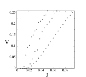
Figure 1: IV characteristics for point pins ($\ast$) and columnar defects, both with random ($\circ$) and periodic ($\triangle$) spatial distribution. Note that $J_{c}$ is almost two times larger for columnar defects compared to point pins. For currents $J>J_{c}$ the randomly distributed columnar pins show a larger resistance than those with a periodic distribution (see text).

The critical current $J_{c}$, which at zero temperature would indicate the location of a non-equilibrium depinning transition, is higher for the columnar pins compared point disorder because of the increased defect correlations. The value of $J_{c}$ is the same for both random and periodic extended defect distributions. The flux line remains localized at few defect sites for $J\leq J_{c}$ as thermal creep happens extremely rarely at $T<<T^{*}$ in the simulations. For currents $J>J_{c}$, the line becomes depinned and we observe that for columnar defects the ensuing voltage is lower for the periodic distribution as compared to the random distribution. This phenomenon can be understood in the following way. Suppose the energy of a flux line inside a columnar pin (say pin 1) of length $L$ is $U_{1}$ and the energy of the flux line in the neighboring pin (pin 2, at a distance $a$ from pin 1) where it arrives after a time $\Delta t(12)$ is $U_{2}$, then $U_{2}-U_{1}\approx-Lf_{L}a$, which is the effective energy barrier between $1$ and $2$ [5]. The transit time is $\Delta t(12)\propto\exp(-\beta Lf_{L}a)$, and hence the mean velocity $v\propto a\exp(\beta Lf_{L}a)$. Let us take a configuration where the three pins $A$, $B$ and $C$ are arranged in a straight line. The distance between $A$ and $B$ is $d_{AB}=a+\delta$ and the distance between $B$ and $C$ is $d_{BC}=a-\delta$. Note $\delta\neq 0$ and $\delta=0$ respectively for random and periodic distribution of the pins. Here the average velocity of hopping between neighboring pins is $\propto\frac{1}{2}[d_{AB}/\Delta t(AB)+d_{BC}/\Delta t(BC)]\propto v[\cosh(\beta Lf_{L}\delta)+\delta\sinh(\beta Lf_{L}\delta)]>v$. Therefore the average velocity of the flux line is less for a periodic defect arrangement as compared to a random distribution. For periodic arrangement of the pins the IV characteristic depends strongly on the orientation of J with respect to the lattice direction, for this determines the effective density of defects encountered by the moving vortex [19].

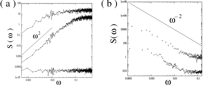
Figure 2: (a) Plot of the power spectrum $S(\omega)$ for $J=0$ for columnar pins at temperatures $T/T^{*}=6.5\times 10^{-4}$ (bottom), $6.5\times 10^{-2}$ (middle) and $T/T^{*}=3.3\times 10^{-1}$ (top). At $T/T^{*}=6.5\times 10^{-4}$, $r_{g}<<b_{0}$ and the voltage noise is essentially thermal (white). At higher temperatures (for $T/T^{*}=6.5\times 10^{-2}$ and $T/T^{*}=3.3\times 10^{-1}$) the flux line starts to ‘feel’ the potential well, rendering the fluctuations over large length scales correlated, as reflected in the nonlinearity in the small $\omega$ behavior of $S(\omega)$. The nonlinearity follows a $\omega^{2}$ (solid line) behavior for small $\omega$ (see text).
(b) Log-log plot of $S(\omega)$ vs. frequency $\omega$ for both columnar $(\triangle)$ and point($\circ$) defects near the depinning threshold at $J\approx J_{c}$. The solid line, given as a guide, has slope $-2$.

The velocity (voltage) noise is calculated by computing the velocity fluctuations about $v_{cm}$. We evaluate the power spectrum $S(\omega)=\overline{\tilde{v}_{x}(\omega)\tilde{v}^{\ast}_{x}(\omega)}$, where $v_{x}(\omega)$ is the Fourier transform of the velocity fluctuation $\tilde{v}_{x}=v_{x}-\langle v_{x}\rangle$, with $v_{x}(t)=[X_{cm}(t+\tau)-X_{cm}(\tau)]/\tau$. The data are averaged over $50$ realizations of disorder for random distributions of defects. At $T=0$ and for $J<J_{c}$, the flux line is bound to one or more pins depending on the type of defects present in the system, and $v_{cm}=0$. For temperatures close to $T=0$ the vortex is still trapped in the defect potential wells, and $r_{g}^{2}=\frac{1}{N}\sum_{i=1}^{N}(r_{\perp i}-\bar{r}_{\perp})^{2}<<b_{0}^{2}$, where $\bar{r}_{\perp}=\frac{1}{N}\sum_{i=1}^{N}r_{\perp i}$. Therefore the line hardly tunnels out of the pins and $S(\omega)$ yields a white (thermal) noise spectrum (Fig. 2 (a)). At higher temperatures, when $r_{g}\approx b_{0}$, long length scale fluctuations can tunnel out of the defects and produce a nonlinear rise as $\propto\omega^{2}$ at small frequencies in $S(\omega)$ (Fig. 2(a)). This is because $S(\omega)$ is an even function, and $S(\omega=0)\approx 0$ (the equality is valid at $T=0$ and in the $L\rightarrow\infty$ limit). The non-white nonlinear part of $S(\omega)$ persists upto larger frequencies for columnar pins as compared to the point defects because of increased correlations induced in the motion of the flux line by the correlated disorder [19]. At temperatures $T>T^{*}$, $r_{g}>>b_{0}$ and the velocity fluctuations are dominated by thermal fluctuations; thus the high-frequency white-noise part of $S(\omega)$ increasingly dominates the spectrum (Fig.  2(a)).

At $J\approx J_{c}$, $S(\omega)$ shows a $1/\omega^{\alpha}$ behavior (Fig.  2(b)), where $\alpha\approx\alpha_{MF}=2$ for almost a decade for both point and columnar defects with deviations at small and large frequencies. This is to be interpreted as a remnant of the zero-temperature depinning transition, representing a non-equilibrium critical phenomenon [21, 22, 23]. Its analysis through a functional renormalization group calculation gives $\alpha=1.5$ for point defects to one-loop order in three dimensions [22, 23], with corresponding mean-field value $\alpha_{MF}=2$. Thus, while our data for lowest frequencies are affected by our finite system size, the $\omega^{-2}$ decay represents the finite-temperature mean-field like behavior to be expected off criticality. The effective exponent $\alpha$ then crosses over to smaller values, perhaps even its true critical value, at larger frequencies. In experiments [4], the broad-band noise (BBN) features show a $\omega^{-\alpha}$ decay with $\alpha\approx 2$ which may similarly be a manifestation of the single-line depinning transition at a finite temperature.

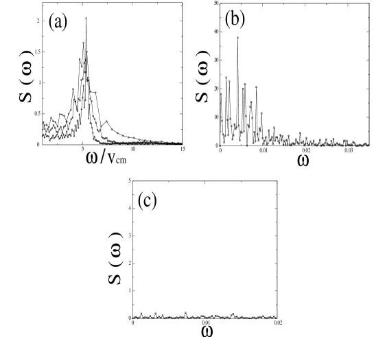
Figure 3: (a) Plot of $S(\omega)$ vs. $\omega/v_{cm}$ for columnar pins arranged in a periodic array for $J=0.05(\circ),\,J=0.07$ (square), and $J=0.09(\triangle)$. The peaks occur at the same scaled frequency $\tilde{\omega}\propto v_{cm}/d$. Note that the width of the peak decreases as $J$ is increased indicating the wider separation between the time scales $\tau_{r}$ and $\tau_{v}$. (b) Plot of $S(\omega)$ vs. $\omega$ for columnar pins distributed randomly in the sample for $J=0.05$ (square). Note the presence of secondary peaks in the spectrum (see text). (c) Plot of $S(\omega)$ vs. $\omega$ for point pins at $J=0.05$ (square). The pronounced peaks present in the case of columnar pins are considerably suppressed (see text).

For currents $J>J_{c}$, two distinct time scales appear in the dynamics — the residence time $\tau_{r}$ which is the duration of the vortices being trapped on the defects, and $\tau_{v}$, the time taken by the flux line to travel between the pins. In the regime where these time scales are well separated and $\tau_{r}<\tau_{v}$, we can expect $\tau_{v}$ to produce pronounced peaks in the velocity noise spectrum. In Fig. 3(a) we plot $S(\omega)$ at different driving currents for the periodic distribution of columnar pins which reveals there is a single peak corresponding to the frequency $\tilde{\omega}\propto v_{cm}/d\propto 1/\tau_{v}$. Note that the width of the peak decreases as the external current ${\bf J}$ increases, which widens the separation between $\tau_{r}$ and $\tau_{v}$. In a random defect distribution (Fig. 3(b)) there would be a distribution of the time scale $\tau_{v}$ around the average value $d/v_{cm}$. Therefore there could be many secondary peaks present in the spectrum arising due to the distribution of $\tau_{v}$ in addition to the principle peak which corresponds to $\tau_{r}\propto d/v_{cm}$. The secondary peaks would eventually diminish as the distribution of the time scales will narrow down at $d/v_{cm}$ with more number of averaging on the defect configurations. Unlike for correlated defects, the time scales $\tau_{r}$ and $\tau_{v}$ are not well separated for point pins. The plot in Fig. 3(c) reveals, as expected, that the peaks are considerably suppressed as compared to the situation for columnar defects (Fig. 3(b)). This difference in $S(\omega)$ between columnar and point pins which results due to the lack of spatial correlation in the $z$ direction for the point disorder can be observed only in a three-dimensional dynamical simulation. It is due to a generic difference between correlated and localized pinning potentials, and should survive even in the presence of interactions between the flux lines. The ensuing absence or presence of the narrow-band noise peaks in the voltage noise spectrum $S(\omega)$, and its specific features, can be utilized as a signature to identify and characterize the type of disorder present and responsible for flux pinning in experimental superconducting samples.

In conclusion we have investigated the three-dimensional dynamics of non-interacting flux lines in the presence of both point and correlated defects. We find the nature of the current-voltage characteristics to depend on the defect correlation and spatial distribution of the pinning centers. The voltage noise spectrum shows pronounced peaks in the case of correlated pins. The difference in the power spectrum at $J>J_{c}$ between columnar and point disorder can serve as a novel diagnostic tool to characterize the pinning centers in superconducting samples.

We would like to thank S. Bhattacharya, A. Maeda, B. Schmittmann, P. Sen, and R. K. P. Zia for valuable discussions. This research has been supported by the National Science Foundation (grant no. DMR 0075725) and the Jeffress Memorial Trust (grant no. J-594).

References

- [1] G. Blatter, M. V. Feigel’man, V. B. Geshkenbein, A. I. Larkin, and V. M. Vinokur, Rev. Mod. Phys. 66 (1994) 1125.
- [2] Y. Togawa, R. Abiru, K. Iwaya, H. Kitano, and A. Maeda, Phys. Rev. Lett. 85 (2000) 3716.
- [3] A. Maeda, T. Tsuboi, R. Abiru, Y. Togawa, H. Kitano, K. Iwaya, and T. Hanaguri, Phys. Rev. B 65 (2002) 054506.
- [4] A. C. Marley, M. J. Higgins, and S. Bhattacharya, Phys. Rev. Lett. 74 (1995) 3029.
- [5] D. R. Nelson and V. M. Vinokur, Phys. Rev. B 48 (1993) 13060.
- [6] D. R. Nelson, Vortex line fluctuations in superconductors from elementary quantum mechanics, in: Proceedings of the NATO Advanced Study Institute on Phase Transitions and Relaxation in Systems with Competing Energy Scales, eds. T. Riste and D. Sherrington (Kluwer Academic Publ., Boston, 1993), p. 95.
- [7] M. Dong, M. C. Marchetti, A. A. Middleton, and V. M. Vinokur, Phys. Rev. Lett. 70 (1993) 662.
- [8] C. J. Olson, C. Reichhardt, and F. Nori, Phys. Rev. Lett. 80 (1998) 2197.
- [9] C. Tang, S. Feng, and L. Golubovic, Phys. Rev. Lett. 72 (1994) 1264.
- [10] C. Reichhardt and C. J. Olson, Phys. Rev. B 65 (2002) 0943011.
- [11] S. Ryu, A. Kapitulnik, and S. Doniach, Phys. Rev. Lett. 71 (1993) 4245.
- [12] S. Ryu and D. Stroud, Phys. Rev. B 54 (1996) 1320.
- [13] A. Schönenberger, A. Larkin, E. Heeb, V. Geshkenbein, and G. Blatter, Phys. Rev. Lett. 77 (1996) 4636.
- [14] D. S. Fisher, Phys. Rep. 301 (1998) 113.
- [15] M. Kardar, Phys. Rep. 301 (1998) 299.
- [16] D. S. Fisher, Low temperature phases, ordering and dynamics in random media, in: Proceedings of the NATO Advanced Study Institute on Phase Transitions and Relaxation in Systems with Competing Energy Scales, eds. T. Riste and D. Sherrington (Kluwer Academic Publ., Boston, 1993), p. 1.
- [17] E. H. Brandt, Phys. Rev. Lett. 69 (1992) 1105.
- [18] M. E. J. Newman and G. Barkema, Monte Carlo methods in Statistical Physics (Clarendon Press, Oxford, 1989).
- [19] J. Das, T. J. Bullard, and U. C. Täuber, in preparation.
- [20] M. Tinkham, Introduction to Superconductivity (McGraw-Hill, NY, 1975).
- [21] O. Narayan and D. S. Fisher, Phys. Rev. B 48 (1993) 7030.
- [22] D. Ertas and M. Kardar, Phys. Rev. Lett. 73 (1994) 1703.
- [23] M. Kardar and D. Ertas, Non-equilibrium dynamics of fluctuating lines, in: Proceedings of the NATO Advanced Study Institute on Scale Invariance, Interfaces, and Non-Equilibrium Dynamics, eds. A. McKane, M. Droz, J. Vannimenus, and D. Wolf (Plenum, New York, 1995), p. 89.